| Issue |
A&A
Volume 600, April 2017
|
|
|---|---|---|
| Article Number | A3 | |
| Number of page(s) | 12 | |
| Section | Planets and planetary systems | |
| DOI | https://doi.org/10.1051/0004-6361/201629801 | |
| Published online | 17 March 2017 | |
Ion acoustic waves at comet 67P/Churyumov-Gerasimenko
Observations and computations⋆
1 Royal Belgian Institute for Space Aeronomy (BIRA-IASB), Avenue Circulaire 3, 1180 Brussels, Belgium
e-mail: This email address is being protected from spambots. You need JavaScript enabled to view it.
2 Swedish Institute of Space Physics, Box 812, 981 28 Kiruna, Sweden
3 Department of Physics, Umeå University, 901 87 Umeå, Sweden
4 Swedish Institute of Space Physics, Ångström Laboratory, Lägerhyddsvägen 1, 75121 Uppsala, Sweden
5 Department of Physics and Astronomy, Uppsala University, 75120 Uppsala, Sweden
6 LPC2E, CNRS, 45071 Orléans, France
7 Physikalisches Institut, University of Bern, Sidlerstrasse 5, 3012 Bern, Switzerland
8 Institut für Geophysik und extraterrestrische Physik, TU Braunschweig, Mendelssohnstr. 3, 38106 Braunschweig, Germany
9 Department of Physics, University of Oslo, Box 1048 Blindern, 0316 Oslo, Norway
10 Laboratoire de Chimie Quantique et Photophysique, Université Libre de Bruxelles, 50 Avenue F. D. Roosevelt, 1050 Brussels, Belgium
Received: 28 September 2016
Accepted: 11 January 2017
Abstract
Context. On 20 January 2015 the Rosetta spacecraft was at a heliocentric distance of 2.5 AU, accompanying comet 67P/Churyumov-Gerasimenko on its journey toward the Sun. The Ion Composition Analyser (RPC-ICA), other instruments of the Rosetta Plasma Consortium, and the ROSINA instrument made observations relevant to the generation of plasma waves in the cometary environment.
Aims. Observations of plasma waves by the Rosetta Plasma Consortium Langmuir probe (RPC-LAP) can be explained by dispersion relations calculated based on measurements of ions by the Rosetta Plasma Consortium Ion Composition Analyser (RPC-ICA), and this gives insight into the relationship between plasma phenomena and the neutral coma, which is observed by the Comet Pressure Sensor of the Rosetta Orbiter Spectrometer for Ion and Neutral Analysis instrument (ROSINA-COPS).
Methods. We use the simple pole expansion technique to compute dispersion relations for waves on ion timescales based on the observed ion distribution functions. These dispersion relations are then compared to the waves that are observed. Data from the instruments RPC-LAP, RPC-ICA and the mutual impedance probe (RPC-MIP) are compared to find the best estimate of the plasma density.
Results. We find that ion acoustic waves are present in the plasma at comet 67P/Churyumov-Gerasimenko, where the major ion species is H2O+. The bulk of the ion distribution is cold, kBTi = 0.01 eV when the ion acoustic waves are observed. At times when the neutral density is high, ions are heated through acceleration by the solar wind electric field and scattered in collisions with the neutrals. This process heats the ions to about 1 eV, which leads to significant damping of the ion acoustic waves.
Conclusions. In conclusion, we show that ion acoustic waves appear in the H2O+ plasmas at comet 67P/Churyumov-Gerasimenko and how the interaction between the neutral and ion populations affects the wave properties.
Key words: comets: general / comets: individual: 67P/Churyumov-Gerasimenko / instrumentation: detectors / methods: analytical / plasmas / waves
Computer code for the dispersion analysis is only available at the CDS via anonymous ftp to cdsarc.u-strasbg.fr (130.79.128.5) or via http://cdsarc.u-strasbg.fr/viz-bin/qcat?J/A+A/600/A3
© ESO, 2017
1. Introduction
The first in situ measurements at a comet were performed in 1985 when the International Cometary Explorer (ICE) spacecraft flew by comet Giacobini-Zinner. The following year several spacecraft probed the environment of comet Halley. A wide variety of plasma waves were detected starting millions of kilometres from the nucleus down to the closest approach at approximately 8000 km for ICE at Giacobini-Zinner and VEGA-2 at Halley (Scarf 1989; Tsurutani 1991). Ion acoustic waves were detected by the ICE spacecraft during its traverse of the bow shock region at Giacobini-Zinner (Scarf et al. 1986), and by the Sakigake spacecraft in the foreshock region upstream of Halley’s comet (Oya et al. 1986).
Ion acoustic waves are compressional waves in a plasma. In the long wavelength limit their frequency is proportional to the wave number. Ion acoustic waves are weakly damped only when the electron temperature Te is much higher than the ion temperature Ti. They are heavily damped if Te ≈ Ti or Te<Ti. For Te ≫ Ti their phase speed can be approximated by the ion sound speed  , where kB is Boltzmann’s constant and mi is the ion mass.
Ion distributions were measured at the comets visited in the 1980s. Richardson et al. (1987) found water-group ions with power law distributions at high speeds that were flattened at low speeds at comet Giacobini-Zinner. Coates et al. (1989) showed that shell-like distributions form when pick up ions undergo pitch angle scattering at comet Halley. This was also observed at comet Grigg-Skjellerup (Coates et al. 1993).
The Rosetta spacecraft (Glassmeier et al. 2007a) has been accompanying comet 67P/Churyumov-Gerasimenko since August 2014 from a heliocentric distance of 3.6 AU down to perihelion at 1.24 AU. The observations reported in this work were made at a heliocentric distance of 2.5 AU on the inbound leg of the orbit around the Sun. In comparison with the comets that were visited in the 1980s, comet 67P/Churyumov-Gerasimenko is a low activity comet. The outgassing rate at 2.5 AU was QH2O ≈ 2 × 1026 s-1 (Simon Wedlund et al. 2016; Hansen et al. 2016), whereas for Giacobini-Zinner it was 2 × 1028 s-1 at the time of the ICE flyby, and 7 × 1029 s-1 for Halley (Tsurutani 1991). The difference in outgassing rate leads to the spatial scales of the comet-solar wind interaction regions being quite different. The observations of scattering of pick up ions at Halley’s comet could be interpreted in terms of Alfvén waves and MHD, as the interaction region was much larger than the gyroradii of the ions. Predictions for comet 67P/Churyumov-Gerasimenko were published by Rubin et al. (2014), who compared the results obtained by MHD and hybrid models.
At 67P/Churyumov-Gerasimenko, 2.5 AU from the Sun, the gyroradius of water group ions picked up by the solar wind was much larger than the size of the interaction region. The interaction between the coma and the solar wind was dominated by mass loading. At the position of the Rosetta spacecraft water ions are accelerated in the direction of a large scale electric field. For cases of low mass loading, the ions were observed to move along the initial part of a cycloid trajectory (Nilsson et al. 2015a). This has been illustrated by simulations (Gunell et al. 2015). When mass loading became more significant, water group ions were seen to move in a more anti-sunward direction than what would be expected in the unperturbed solar wind (Nilsson et al. 2015b; Behar et al. 2016b). Behar et al. (2016a) compared simulations with measurements at 67P/Churyumov-Gerasimenko over a range of heliocentric distances. An illustration of the interaction between the solar wind and the comet is shown in Fig. 1.
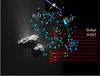 |
Fig. 1 Illustration of particle motion at 67P/Churyumov-Gerasimenko, showing outgassing of neutral water molecules, the beginning of the H2O+ trajectories, and deflection of solar wind ions. During the observations reported in this paper the position of the spacecraft was 28 km from the comet, which was 2.5 AU from the Sun. Schematic of solar wind deflection adapted from Behar et al. (2016a). Photo of nucleus and spacecraft: ESA – European Space Agency. |
Due to the different scales at high and low activity comets, the physical processes at work are different. However, also high activity comets go through a low activity phase, which may happen farther away from the Sun than for low activity comets. A survey of the plasma environment of 67P/Churyumov-Gerasimenko was performed by Odelstad et al. (2015), who reported electron temperatures around 5 eV. Low frequency wave activity – the peak of the spectrum at approximately 40 mHz – was discovered by Richter et al. (2015), observed simultaneously at two points by Rosetta and the Philae lander (Richter et al. 2016), and has been interpreted in terms of a modified ion-Weibel instability (Meier et al. 2016).
In this paper, we report observations of ion acoustic waves by the Rosetta spacecraft in the plasma 28 km from the nucleus of comet 67P/Churyumov-Gerasimenko on 20 January 2015. We measure the ion distribution function and the electron density and temperature. Based on these quantities we compute dispersion relations that are compared to the wave observations. Then, we discuss the relationship between the wave observations, the ion distributions, and the neutral gas. In Sect. 2 we derive ion distributions from the Ion Composition Analyzer of the Rosetta Plasma Consortium (RPC-ICA) data (Nilsson et al. 2007) and compare the density estimates obtained by the Langmuir probe (RPC-LAP; Eriksson et al. 2007), the Mutual Impedance Probe (RPC-MIP; Trotignon et al. 2007), and the RPC-ICA instruments; in Sect. 3 we present wave observations by the RPC-LAP instrument; in Sect. 4 we compute dispersion relations based on the ion distributions and electron density and temperature measurements; in Sect. 5 we treat the relationship between the ion populations and the neutral gas density measured by the Comet Pressure Sensor (COPS) of the Rosetta Orbiter Spectrometer for Ion and Neutral Analysis (ROSINA) instrument (Balsiger et al. 2007); and in Sect. 6 the conclusions are discussed.
2. Ion distributions and densities
2.1. Instrument
RPC-ICA is mounted on the Rosetta spacecraft (Nilsson et al. 2007). It measures the differential particle flux of ions in 16 sectors in its nominal viewing plane, as shown schematically in Fig. 2.
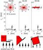 |
Fig. 2 Geometry of the observations. Panels a)–c) show the viewing directions, that is, the centres of the fields of view, for the RPC-ICA instrument projected onto the plane containing the comet to spacecraft direction and the CSEQ x direction for times 08:00, 16:24, and 20:46 in panels a)−c), respectively. The nucleus of the comet is located at the origin of the coordinate system. For the same times, panels d)–f) show the orientation of the spacecraft and the ROSINA COPS instrument with respect to the gas flow from the nucleus, which is shown by the black arrows. |
The instrument scans a range of elevation angles with respect to that plane. A complete sweep over all energies and elevation angles takes 3 min 12 s.
Figure 3a shows the sum of the differential particle flux from all directions within the field of view as a function of time and E/q for the ions, where E is the kinetic energy and q the charge of the ion. In this ion energy spectrum from 20 January 2015 three ion species can be identified: alpha particles, which have E/q values above 1 kV; protons, appearing at E/q ≈ 600 V, and water ions at lower values of E/q. The bulk of the water ions are formed close to the spacecraft and appear in Fig. 3a at E/q ≲ 10 V. The energy scale in Fig. 3a has been compensated for an instrumental offset and for the spacecraft potential. That there is an offset in the energy table was found by Nilsson et al. (2015a) when measurements started at the comet. The voltage of the electrostatic analyser differed from what had been measured in the laboratory before launch. The value of the offset can now only be determined using the instruments onboard the spacecraft. The lowest energy ions that we observe come in at a tabulated energy of 25.5 eV. Of this, the offset is approximately Voffset = −9 V and what remains is assigned to the spacecraft potential Vsc ≈ −16.5 V. This is confirmed by comparison with Langmuir probe data, although an uncertainty remains as the Langmuir probe may have an offset of its own. The −16.5 V spacecraft potential is consistent with negative spacecraft charging from a plasma where the electron temperature is 5–10 eV as seen in Fig. 3c. There is also a tail of H2O+ ions reaching energies of a few hundred eV. These have been created in ionisations farther away from the spacecraft and have had time to be accelerated before they were observed (Nilsson et al. 2015a,b).
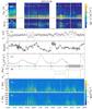 |
Fig. 3 Overview of the observations by instruments on board the Rosetta spacecraft on 20 January 2015. a) Ion energy spectrum measured by RPC-ICA. The colour coded quantity is the differential particle flux summed over all viewing directions. The energy scale has been adjusted for Vsc and Voffset. b) Differential particle flux of hot water ions (9 eV ≲ E ≲ 23 eV when E is adjusted for offset and spacecraft potential) for the different sectors of the RPC-ICA instrument. c) Electron temperature observed by RPC-LAP. d) Magnitude of the magnetic flux density B seen by RPC-MAG. e) Neutral gas density measured by ROSINA-COPS. f) Angles between the coordinate axes of the spacecraft frame of reference and the direction to the nucleus of the comet. g) Power Spectral density of the current to Langmuir probe 1 in the frequency range 200 Hz <f ≤ 1450 Hz. h) Power Spectral density of the current to Langmuir probe 2 for 200 Hz <f ≤ 1450 Hz. Periods when the ROSINA-COPS measurements were affected by the spacecraft pointing are marked in grey at the bottom of panel e) and the top of panel f). The spikes in the neutral density at 03:54, 14:00, and 23:31 (shown in grey in panel e)) are due to wheel off-loading manoeuvres. The RPC-ICA instrument (panels a) and b)) was off during these manoeuvres. |
2.2. Measured distributions
To compute a water ion distribution function from the RPC-ICA data we consider one complete sweep in energy and elevation angle for all sectors and mass channels. This takes 3 min 12 s, which thus is the temporal resolution at which we know the distribution function. Water ions are selected by considering the E/q< 350 V range only. We collect the contributions to the phase space density (Fränz et al. 2006; Lavraud & Larson 2016) 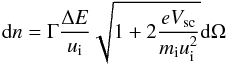 (1)on a three-dimensional grid in velocity space. In Eq. (1) Γ is the differential particle flux; ΔE the width of the energy bin; ui = (2(E + eVoffset)/mi)1/2 the ion speed corresponding to the central energy of the bin, corrected for the offset as discussed below; mi the ion mass; Vsc the spacecraft potential, and dΩ is the solid angle of the field of view. The factor
  has been introduced to compensate for the effects of the sheath that surrounds the negatively charged spacecraft (Lavraud & Larson 2016). The velocity space position of the density element in Eq. (1) is determined by the viewing direction of the respective sector and elevation angle and by the energy of the electrostatic analyser. The energy value is compensated for the offset and the spacecraft potential to obtain vi, the speed of the ion before it was accelerated in the sheath surrounding the spacecraft. We have
  (2)where E is the energy setting for the centre of the energy bin.
The three-dimensional distribution function is integrated over one dimension to obtain f(vχ,vζ), the two-dimensional projection in one plane. The orientation of this plane is chosen so that it contains as much as possible of both the thermal and the accelerated ions, and the plane is rotated to place the accelerated ion tail on the positive horizontal axis. Three examples for the times 08:00, 16:24, and 20:46 are shown in panels a–c) of Fig. 4.
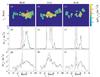 |
Fig. 4 Water ion distribution functions observed at 08:00 (left column), 16:24 (mid column), and 20:46 (right column) on 20 January 2015. Panels a)–c) show the two-dimensional projection of the distribution function on a plane in velocity space. Panels d)–f) show the one-dimensional projection of the distribution functions on the horizontal axis of panels a)–c). Panels g)–i) show the same one-dimensional projection on a logarithmic vertical scale. The black curves show the data. The red, blue, and green curves show three different functions used as fits to the data. Corrections for the instrument offset and spacecraft potential have been applied. Densities and temperatures for the model curves are shown in Table 1. |
The sum of the instrumental offset and the spacecraft potential that appears in Eq. (2) can be determined empirically from the data. We find that, for the distributions in Figs. 4a–c, a value of Vsc + Voffset = −25.5 V closes the hole in the distribution that would appear at ui = 0 if this compensation for the offset and spacecraft potential were not applied.
The two-dimensional distributions shown in Figs. 4a–c are integrated over vζ and we obtain f(vχ), the one-dimensional projection of the distribution function, which is shown by the black curves in the lower six panels of the figure. In panels d–e) the vertical scale is linear and panels g–i) show the same quantity on a logarithmic scale. The red, green, and blue curves represent different ways of fitting simple pole expansions to the observational data. This will be used in Sect. 4.
The RPC-ICA field of view does not cover all directions. The elevation angle is scanned over ± 45° from the nominal entry plane of the instrument. This angular range is somewhat narrower and the angular resolution coarser for ion energies below 100 eV. For the lowest energies reported in this paper the elevation angle range covered is 44° wide, that is to say, about half of the nominal range. Also, some of the field of view is obscured by the spacecraft, and the trajectories of low energy ions may be affected by electric fields in the near-spacecraft environment. Thus, there are parts of the ion distribution that are not sampled by the instrument. To arrive at a realistic approximation that can be used in the dispersion relation calculations, assumptions must be made about this unobserved part. The assumption behind the distributions that are shown by the red curves in Fig. 4 is that the central part of the distribution, vi ≲ 7−9 km s-1 is isotropic. For this isotropic part the maximum flux observed for each energy bin is assumed to be the flux incident from all directions. Integrating that distribution over all velocities yields the bulk density.
2.3. Modelled distributions
We model the distribution by a sum of approximate Maxwellians, described by simple pole expansions. The thermal spread of the bulk of the water ion population is given by the temperature that fits the slope of the central part of the distribution as illustrated in Figs. 4d–f. The model distributions are described in more detail in Sect. 4.2 and in Appendix A. For the faster ions in the tail or beam it is assumed that there are no contributions other than those that are observed. The parameters thus obtained are shown in Table 1.
The direction from whence the beam enters the detector corresponds mainly to sectors 7 and 8 and due to the elevation angle scan it remains in the field of view when the spacecraft turns as shown in Figs. 2a–c.
Due to the limitations in angular coverage and resolution, particularly at low energies, density estimates that are based on RPC-ICA measurements alone can be uncertain. We have therefore included three different distribution function estimates for each of the three times in Fig. 4. The distributions shown by the red curves in Figs. 4d–i are based on RPC-ICA data only; the distributions represented by the dashed green curves also take information obtained from Langmuir probe current–voltage characteristics into account; and the blue curves are obtained assuming a higher bulk density in order to produce dispersion relations in agreement with the power spectral densities observed by the Langmuir probe. At all three times, the assumed density is much lower for the red curve than for the green and the blue curves. The blue curves are not much different from the green ones in Fig. 4, but, as seen in Table 1, the electron temperatures differ between the two sets, affecting the dispersion relation calculations in Sect. 4.
At 16:24 the two-dimensional distribution shown in Fig. 4b shows a ring-shaped region, which indicates that there is a higher temperature isotropic distribution present. In the other two cases only faint traces of such a ring-shaped region can be seen. In order to model this difference a higher bulk ion temperature has been assumed for the green and blue curves at 16:24, while it remains low for the times 08:00 and 20:46. In Sect. 4 dispersion relations computed for the alternative distributions will be compared to wave data, and that can be used to determine which assumption is the more realistic in each case.
2.4. Density estimates: inter-instrumental comparison
A density estimate can be obtained by integrating the ion distribution function over all three velocity dimensions. The red curve density in Table 1 was obtained in this way. The difference between this density estimate and the one derived from the Langmuir probe, which is tabulated for the green curve in Table 1, is relatively large. It is therefore useful to choose an interval where density data from RPC-LAP, RPC-ICA, and the mutual impedance probe (RPC-MIP) are available simultaneously to cross-calibrate the instruments and assess the accuracy of the different methods. Reliable RPC-MIP densities and RPC-LAP wave spectra are not always available at the same time, especially during the low activity phase of the comet when RPC-MIP density estimates are mainly retrieved in the long Debye length (LDL) mode (Trotignon et al. 2007). Therefore 19 January 2015, the day before the one which is the primary subject of this investigation, was chosen for cross-calibration purposes. Figure 5
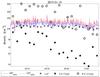 |
Fig. 5 Comparison of densities derived from RPC-ICA measurements to those from RPC-LAP and RPC-MIP. The blue and red lines show the minimum and maximum RPC-MIP plasma density estimates, respectively. Estimates based on RPC-LAP data are marked “×”. The two sets of estimates derived from RPC-ICA data assuming the ion distribution to be isotropic for vi ≲ 7 km s-1 and vi ≲ 12 km s-1 are marked “∗” and “°”, respectively. The data sets were recorded on 19 January 2015. |
shows density estimates obtained from RPC-ICA, RPC-LAP, and RPC-MIP spectrum recorded during a period on 19 January 2015, when RPC-MIP estimated a stable plasma density of approximately 150 cm-3. The RPC-MIP density estimates are derived by evaluation of the complex (amplitude and phase) active mutual impedance spectra when RPC-MIP was operated in the LDL mode.
For the estimates based on RPC-ICA data only the central part of the ion distribution function has been assumed to be isotropic. Estimates using two different limits for the isotropic part are shown in Fig. 5, namely vi ≲7 km s-1 and vi ≲ 12 km s-1. The 12 km s-1 limit gives an agreement with RPC-MIP within a factor of three. The 7 km s-1 limit gives an underestimate of the density, and the difference is large for some of the data points. Most of the ion density is located in the low energy part of the distribution, which is the most difficult to measure accurately, and it is also the most affected by the potential structure that surrounds the negatively charged spacecraft.
Examination of Langmuir probe current–voltage characteristics yields electron temperatures in the 6–10 eV range with a mean value of 7.3 eV during the interval in Fig. 5. The density estimates obtained from the Langmuir probe are somewhat lower than those obtained by RPC-MIP as Fig. 5 shows. However, the difference between the data points is not overly large, and knowing that the density is likely to be underestimated, a correction could be applied. For these observations we assume that the most accurate estimate of the plasma density is the one derived from the plasma frequency observed by RPC-MIP. In the absence of RPC-MIP data, as for example on 20 January, RPC-LAP data should provide a more accurate density value than RPC-ICA data.
3. Wave observations
Throughout the day of 20 January 2015, the two Langmuir probes recorded 535 time series of 1600 samples each at a sampling frequency of 18750 Hz. Thus, each time series is 85.3 ms long. The probes were kept at a constant potential, probe 1 at +30 V and probe 2 at −30 V with respect to the spacecraft, and the current to each of the probes was recorded. Power spectral densities for the two probes are shown in the left column of Fig. 6 for times 08:00, 16:24, and 20:46.
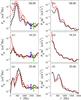 |
Fig. 6 Panels a), c), and e): power spectral densities of the currents to the Langmuir probes at 08:00, 16:24, and 20:46 on 20 January 2015. The red lines show probe 1 and the black lines probe 2. The dashed lines show lower frequency resolution, where data points taken while the RPC-MIP instrument was running have been removed. The error bars show the 95% confidence intervals for the solid curves in blue and the dashed curves in green. Panels b), d), and f) power spectral densities divided by ω2. |
Noise from the RPC-MIP instrument can potentially be picked up by the probes, distorting the measured spectrum. The two instruments are synchronised so that for each 8 ms period of RPC-LAP data, RPC-MIP is operating during the first 2 ms. The power spectral density may be computed for the 6 ms interval when RPC-MIP is off, but the short duration of the 6 ms segments limits the frequency resolution. Each 6 ms segment comprises only 113 samples. In Fig. 6 the dashed curves have been computed by averaging the power spectral densities obtained in all 6 ms segments unperturbed by RPC-MIP during one complete 1600 sample (85.3 ms) time series. The solid curves are computed from the complete time series using Welch’s method (Welch 1967), averaging segments of 256 samples with 65% overlap. The confidence intervals for a 95% confidence level are shown by error bars in panels a), c), and e). The blue error bars correspond to the solid curves and the green bars to the dashed curves. The upper and lower limits of the confidence intervals are frequency-independent factors multiplied by the value of the power spectral density. Since the vertical scales are logarithmic, this means that the error bars have the same size for all frequencies. It is seen in the figure that for frequencies above 200 Hz, the agreement between the dashed and solid lines is good to the extent that the frequency resolution allows. Below 200 Hz the difference between the curves is larger. In panels g) and h) of Fig. 3, which show all 535 probe spectra recorded during the day, the same method as for the solid lines in Fig. 6 has been used in order to achieve a higher frequency resolution, but the spectrum is only shown for 200 Hz <f ≤ 1450 Hz.
The amplitude of the signals obtained by the two probes are of the same order of magnitude, in spite of probe 1 being biased 60 V above probe 2. In Fig. 6e the peak amplitude of the signal from probe 2 is even higher than that from probe 1. The DC current to the positively biased probe 1 is carried by electrons, while the DC current to probe 2 is dominated by photo emission. If the observed oscillations were due to particle currents proportional to the plasma density, one would expect much higher amplitudes to be observed by probe 1 than probe 2. Since that is not the case, we conclude that, for frequencies above 200 Hz, the observed current is a displacement current due to the capacitive coupling of the probe to the plasma.
Capacitively coupled double probes have been used to measure AC electric fields in laboratory plasmas (Torvén et al. 1995). It was found that the measured current is proportional to the derivative of the wave electric field with respect to time, dEw/ dt, and to the capacitance between the two probe tips. Similar circuit models have been used to model the capacitive regime of probes on spacecraft (Eriksson et al. 1997). The presence of the spacecraft modifies the electric field in the vicinity of the probe and the spacecraft itself from what it would have been in the unperturbed plasma. The signal that is picked up depends on the direction of the wave field, and that is unknown. Thus, for the wave analysis in this paper, we have at our disposal a relative, but not absolute, measurement of dEw/ dt.
In order to display a quantity that is proportional to the power spectral density of Ew, instead of dEw/ dt, the power spectral densities of the current have been divided by ω2 to obtain PII/ω2, which is shown in the right column of Fig. 6. Dividing by ω2 amplifies low frequency noise, changing the shape of the curve also in the absence of a wave signal. The spectrum obtained at 08:00, panels a) and b), has its main peak just below 500 Hz, and a peak at the second harmonic can also be seen. The spectrum recorded at 20:46 (panels e) and f)) is similar in shape, except that there is no discernible second harmonic, and the peak is just above 500 Hz. The spectrum measured at 16:24 (panels c) and d)) is not above the noise floor. There is a noise floor at PII = (2−4) × 10-5 nA2/Hz above f = 300 Hz, increasing to about 10-4 nA2/Hz at f = 200 Hz. This is also seen in panels g) and h) of Fig. 3. Below f = 200 Hz the spectrum obtained at 16:24 is also at the noise floor level, as seen from the dashed curves in Fig. 6c.
While we cannot make a precise determination of the electric field, an order of magnitude estimate can be made. For the spectra that are above the noise level, that is to say, those obtained at 08:00 and 20:46, PII/ω2 ≈ 10-28 A2 s-3 at the peak near 500 Hz. Ideally, one would model a probe by its vacuum capacitance, which for a probe of 2.5 cm radius is 2.8 pF. We take this as an upper limit. In the presence of the spacecraft, the circuit would be better modelled by a lower value, of the order of 1 pF. The effective length over which the wave potential is applied depends on the direction of the field with respect to the probe-to-spacecraft direction, and we take it to be (1–2) m. Thus, the power spectral density of the electric field should be in the approximate range of (10-6−10-4) V2 m-2/ Hz.
4. Wave dispersion analysis
In this section we present dispersion relations and fluctuations for the distributions presented in Sect. 2.
4.1. Basic conditions and assumptions
We assume that all water group ions are H2O+ ions. These ions may be converted to H3O+ in ion-neutral collisions. Fuselier et al. (2016) measured the ratio of the H3O+ to H2O+ concentrations and found that either species may dominate over the other. Since the masses of these two ions are 19 u and 18 u respectively, the mass ratio is approximately 1.06, and the corrections of speeds and ion plasma frequencies are less than 3%, as both these quantities depend on the square root of the ion mass. Gledhill & Hellberg (1986) showed that for mass ratios less than 3 the wave modes associated with one species change continuously into those of the other as their relative densities change. In our case these two sets of wave modes were already close to one another. Thus, even if a substantial part of the ions are H3O+ ions, the effect on the wave analysis would amount only to a small correction and would not qualitatively change the results.
We use a single thermal distribution to model the electrons with a temperature obtained by the Langmuir probe. It is possible that a fraction of the electrons belong to a hotter – suprathermal – distribution. Such suprathermal electrons, with kinetic energies of approximately 100 eV and densities at a level of 10% of the thermal densities, were observed at comet 67P/Churyumov-Gerasimenko by Madanian et al. (2016). While the presence of suprathermal electrons can support electron acoustic waves, a suprathermal to thermal density ratio of above 0.2 would be required (Mace & Hellberg 1990). Even in the hypothetical case when 90% of the electrons are suprathermal and the hot to cold temperature ratio is 100, the weakly damped regime is confined to frequencies above 0.1fpe (Mace & Hellberg 1990). This is far above the ion plasma frequency, and therefore these waves would not interfere with the ion acoustic waves.
The magnetic field was measured by the RPC-MAG instrument (Glassmeier et al. 2007b) and was of the order of 10 nT throughout the day of observations, as Fig. 3d shows. This corresponds to a cyclotron frequency of approximately 0.01 Hz for water ions, and the gyro radius for a H2O+ ion at an energy of 1 eV is approximately 60 km, which is much larger than the phenomena considered here. For pickup ions that are accelerated to much higher energies the gyro radii are even larger. The electron cyclotron frequency is in the approximate range of the observed waves, fce = 280 Hz for | B | = 10 nT, but we can rule out the presence of electron cyclotron waves since the temporal evolution of the wave frequency does not follow the B-field magnitude. Thus, the plasma is assumed to be unmagnetised. Furthermore, we consider it to be one-dimensional along the direction of the water ion beam or tail.
4.2. Theory
The computational method is based on simple pole expansions of the distribution functions (Löfgren & Gunell 1997; Tjulin et al. 2000; Gunell & Skiff 2001, 2002; Tjulin & André 2002). We first review the basic ideas behind this method and the equations that we use in this paper. A distribution function can be written as a sum of several components each described by a “simple pole expansion” of the form (Löfgren & Gunell 1997) ![Mathematical equation: \begin{eqnarray} \label{eq-expansion} &&f(v) = M(v)T(v),\nonumber\\ &&M(v) = \left[1+ \frac{\left(v-v_\mathrm{d0}\right)^{2}}{2v_\mathrm{t}^{2}}+\ldots+ \frac{1}{m!}\left(\frac{\left(v-v_\mathrm{d0}\right)^{2}}{2v_\mathrm{t}^{2}}\right)^{m} \right]^{-1},\\ &&T(v) = \left[1+\left(\frac{v-v_\mathrm{d1}}{v_\mathrm{c}}\right)^{2n} \right]^{-1},\nonumber \end{eqnarray}](/articles/aa/full_html/2017/04/aa29801-16/aa29801-16-eq83.png) (3)where M is the reciprocal of a Taylor expansion of
(3)where M is the reciprocal of a Taylor expansion of  , vd0 is the average drift velocity and vt0 is the thermal speed. M approaches a drifting Maxwellian as m tends to infinity. When only a few terms are included in the expansion, M(v) is an approximate Maxwellian for small values of | v |, but with thicker tails for large | v | values. The factor T(v) is used to introduce cutoffs in the tail of M(v) at v = vd1 ± vc. The larger the number n is, the sharper this cutoff will be. Asymmetries can be introduced by choosing a vd1 that is different from vd0. This is illustrated in Appendix A.
Functions of the form described by Eq. (3) can be written as a sum involving simple poles and residues in the complex phase velocity plane: 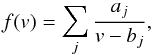 (4)where bj are the poles of the distribution function and aj are the residues at those poles. In a plasma composed of different species, α, the dielectric function is (e.g. Krall & Trivelpiece 1973)
 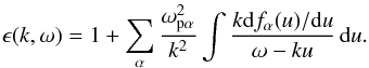 (5)The sum of distributions in Eq. (5) includes all components that form the ion distributions as well as the electrons. In Sect. 4.3 we shall show that the influence of solar wind ions is negligible, and that only electrons and water group ions are important for the observed waves. Each component fα is normalised and weighted with its plasma frequency squared,
  , when forming the sum in Eq. (5). We integrate in the complex plane, closing the integral path in the upper half plane, and obtain (Gunell & Skiff 2002)
 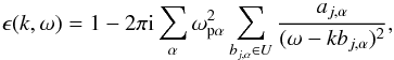 (6)where U denotes the upper half-plane. Dispersion relations for the normal mode of the plasma are found by assuming a real value for k and finding the complex ω that satisfies
  (7)Equation (6) can be arranged, expressing ϵ(k,ω) as a polynomial in ω/k, whereafter Eq. (7) is solved by standard root finders (Löfgren & Gunell 1997; Gunell & Skiff 2001). However, if the modulus | bj,α | differs significantly between the poles, this becomes an ill-posed problem. Therefore, in this work, Eq. (7) is solved by numerically finding the solutions that minimise | ϵ(k,ω) | 2. In the convention used here, the imaginary part of ω is positive for damped modes and negative for unstable modes. Computer code for computing dispersion relations has been deposited with this article as supplementary material.
4.3. Negligibility of the solar wind contribution
In Fig. 7a
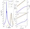 |
Fig. 7 Dispersion relations at 08:00 on 20 January 2015. a) Distribution functions for cometary water ions (solid blue curve) and solar wind protons (dash-dotted orange curve) and alpha particles (dashed black curve). b) Real part of ω as a function of wave number. c) The imaginary part of ω as a function of wave number. In this case γ> 0 for all three curves, which means that these modes are damped. The blue curves represent the same mode as the blue curves in Fig. 8. |
model distribution functions are shown for cometary water ions (solid blue curve) and solar wind protons (dash-dotted orange curve) and alpha particles (dashed black curve). We combine these three populations to form ϵ(k,ω) according to Eq. (6). Then, the solutions to Eq. (7) are found. In panels b) and c) the dispersion relation and the damping rate are shown, respectively, for the ion acoustic mode (blue curve) and the beam modes associated with the solar wind protons (dash-dotted orange curve) and alpha particles (dashed black curve). The ion acoustic mode shown here is the same as the one shown by the blue curve in Fig. 8. It is not affected by the presence of the solar wind ion species, because the density of these is insignificant in comparison with the water ion density. Also, the velocity of the solar wind ions is above 300 km s-1, which is out of resonance with the ion acoustic speed that is only about 6 km s-1. The proton and alpha particle beam modes are heavily damped, with damping rates three orders of magnitude above that of the ion acoustic mode. Thus, the solar wind ions can be neglected, and we shall consider only H2O+ ions.
4.4. Water ion waves
We have applied this method to the distributions obtained at 08:00, 16:24, and 20:46 on 20 January 2015. In each of those cases, dispersion relations were calculated for three different parameter sets detailed in Table 1 and with distributions shown by the red, green, and blue curves in Fig. 4. The ion properties of each curve are described in Sect. 2. For red and blue curves an electron temperature of kBTe = 7 eV has been used. Figure 3c shows that this was the approximate average temperature during the day, although the values scatter somewhat both above and below 7 eV. For the green curve we used the value obtained from examination of Langmuir probe current–voltage characteristics at the three times considered.
Figure 8
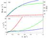 |
Fig. 8 Dispersion relations at 08:00 on 20 January 2015. a) Real part of ω as a function of wave number. b) The imaginary part of ω as a function of wave number. For growing modes γ< 0 and for damped modes γ> 0. The red, blue, and green curves correspond to the distribution functions shown in Figs. 4d and g by the red, blue, and green curves, respectively. |
shows the dispersion relations for the three alternative distribution functions used to approximate the ion measurement at 08:00 on 20 January 2015 shown in, Fig. 4 with parameters in Table 1. The damping rate γ shown in panel b) is defined as the imaginary part of ω, which means that damped modes have γ > 0 and growing modes have γ < 0. Only the ion acoustic mode is shown, as it is the least damped or most unstable mode for all three parameter sets. For the ion acoustic mode, ω is proportional to k for small k values, and the curve flattens out as it approaches the ion plasma frequency, which is approximately 500 Hz for water ions with a density of 108 m-3. In the low bulk density case (red curves) the beam becomes relatively more important, and this makes the ion acoustic mode unstable for small values of k. The minimum of the red curve in Fig. 8b gives the most unstable point. This point corresponds to a frequency of 22 Hz. For higher frequencies the damping rapidly increases. This is inconsistent with the observation in Fig. 6 that there is a peak in the spectrum near 500 Hz, which is higher than the ion plasma frequency for the low-density parameter set. When a higher bulk density is assumed, as shown by the green and blue curves, ion acoustic waves are weakly damped over a larger frequency range including the frequency at which the peak appears in Fig. 6. The blue curve, with its somewhat higher ion plasma frequency, shows the best agreement with the spectrum in Fig. 6. At the peak, f ≈ 450 Hz, the wavelength of the ion acoustic waves is λ ≈ 10 m. The distribution function corresponding to this blue curve is shown by the blue curves in Figs. 8 and 4d, g. It is based on a density ne = 1.65 × 10⁸ m-3, which we take as the estimate obtained from the comparison between the computed dispersion relation and the observed spectrum. This density estimate is higher than that obtained from the Langmuir probe sweeps by approximately a factor of 2.
Figure 9
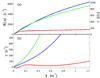 |
Fig. 9 Dispersion relations at 16:24 on 20 January 2015. a) Real part of ω as a function of wave number. b) The imaginary part of ω as a function of wave number. For growing modes γ < 0 and for damped modes γ > 0. The red, blue, and green curves correspond to the distribution functions shown in Fig. 4e and h by the red, blue and green curves, respectively. |
shows the dispersion relations for the three alternative interpretations of the ion distribution obtained at 16:24. These differ in both density and temperature, the distributions shown by the green and blue curves being denser and having higher temperatures as seen in Fig. 4 and Table 1. The wave modes shown are ion acoustic modes in all cases. In the higher temperature and density cases these waves are heavily damped. The damping rates for the blue and green curves in Fig. 9b are significantly higher than those for the blue and green curves in Fig. 8b. The low density and temperature distribution is unstable with the most unstable point at 48 Hz. Since no waves were seen above the noise floor in Figs. 6c and d, the higher temperature and density interpretations (blue and green curves), which yield highly damped waves, are in better agreement with the observations than the other interpretation represented by the red curve. To completely rule out the red curve prediction, we consider the spectrum at low frequencies in Fig. 6c, using the dashed curves, as discussed in Sect. 3. The spectrum is no higher there than it is in Fig. 6a, where a wave mode peaking at higher frequencies can be identified. Since the Langmuir probe spectrum is below the noise floor for the time 16:24 we cannot distinguish between the blue and the green curves, to make a density estimate.
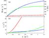 |
Fig. 10 Dispersion relations at 20:46 on 20 January 2015. a) Real part of ω as a function of wave number. b) The imaginary part of ω as a function of wave number. For growing modes γ < 0 and for damped modes γ > 0. The red, blue, and green curves correspond to the distribution functions shown in Figs. 4f and i by the red, blue, and green curves, respectively. |
Figure 10 shows the dispersion relations for the low (red) and high (blue and green) density interpretations of the ion distribution obtained at 20:46 on 20 January 2015. In all three cases Te ≫ Ti, and the ion acoustic mode is weakly damped. For the red curve the damping is only weak for small values of k, it rapidly increases with increasing k, and frequencies near the observed peak, f ≈ 590 Hz in Figs. 6e and f, are never reached. Of the two higher density interpretations the blue curve, corresponding to ne = 2.1 × 10⁸ m-3, produces the better agreement with the peak in the Langmuir probe spectrum. This is higher than that obtained from the Langmuir probe sweeps by about a factor of 3. The wavelength of these waves is estimated to be λ ≈ 6 m.
It is worthwhile to estimate how much a Doppler shift could modify these results. The whole ion population could possibly be drifting at about vi = 1 km s-1, which is approximately the speed at which the neutral gas expands away from the nucleus and which is small enough to escape detection in the ion measurements. For the red curves in Figs. 8 and 9 we have k ≈ 0.05 m-1. The Doppler shift would be Δf = kvi/ (2π) ≈ 8 Hz. This is lower than the frequencies of the unstable modes calculated above, that is to say, 22 Hz for the red curve in Fig. 8 and 48 Hz for the red curve in Fig. 9. Thus a Doppler shift does not change the conclusion that the low density distributions described by the red curves are inconsistent with the wave observations. For the green and blue curves in Figs. 8−10, k ≈ 0.5 m-1 at f = 400 Hz. In this case the Doppler shift would be Δf ≈ 80 Hz. This is enough to make it difficult to determine which of the distributions represented by the green and blue curves best models the observations, but it does not change the nature of the interpretation.
5. Ion–neutral relationship
The presence of a warm ion population, as in panels b), e), and h) of Fig. 4, leads to an increased damping of ion acoustic waves, as seen in Fig. 9. The damping increases because when Ti gets closer to Te, the ion thermal speed approaches the phase velocity of the ion acoustic waves. In panel b) of Fig. 3 the flux in the energy range 9 eV ≲ E ≲ 23 eV is shown for the different sectors of the RPC-ICA instrument. Here E has been adjusted for the offset and spacecraft potential. When present, a warm and isotropic ion distribution should contribute to the flux in most sectors. One would always expect a lower flux into sectors 10−15 that are partially obscured by the spacecraft body (Nilsson et al. 2007). The measured flux into sector 1 is low due to the low sensitivity of that sector. At times when there is a significant flux in a wide range of sectors the Langmuir probe spectra in Fig. 3g and h show less wave activity: around 02:00, from about 09:30 to 11:00, from 16:00 to 18:00, and after 22:00. Ion acoustic waves are heavily damped in the presence of the warm ion populations, as illustrated by the dispersion relations in Sect. 4. The temperature of the warm ions is approximately 1 eV determined by fitting the green and blue curves to the observed distribution in Fig. 4.
The ROSINA-COPS instrument (Balsiger et al. 2007) contains the Nude Gauge, an ionisation gauge in which a current, which is proportional to the density of the neutral gas emitted by the comet, is drawn between a hot filament and an anode. This neutral density is shown in Fig. 3f. The sensitivity is computed from the raw data assuming the sensitivity for water, and a correction for the contribution from outgassing from the surface of the spacecraft has been applied by subtracting 1.1 × 10¹² m-3. The dropout in neutral density between 18:52 and 22:44 is caused by a slew manoeuvre that turned the side of the spacecraft where the ROSINA-COPS instrument is mounted away from the comet, as shown in Fig. 2f. Neutrals cannot reach the instrument except through collisions. With Nn = 4 × 10¹³ m-3 and T = 100 K the mean free path for elastic collisions between water molecules is Λ = 1.07 × 10¹⁸ m-2(T/ 300 K)0.6/Nn = 1.4 × 10⁴ m (Crifo 1989), which is much larger than the spacecraft dimensions, and the flow can be considered collisionless. The angles between the spacecraft to comet direction and the three axes of the spacecraft reference frame are shown in Fig. 3f. The spacecraft turned by a smaller angle between 14:30 and 18:00. This manoeuvre did not affect the neutral density measurement as the sensor remained in the gas flow as Fig. 2e shows.
The three largest neutral density peaks, at approximately 10:20, 17:00, and 22:50 in Fig. 2f, coincide with periods when warm ions are observed. The situation was less clear early in the day, when the neutral density was in the range 1 × 10¹³ m-3 ≲ Nn ≲ 2 × 10¹³ m-3. The 1 eV temperature of the warm ions is much greater than the neutral temperature of a couple of hundred kelvins obtained in published models (e.g. Fougere et al. 2013; Bieler et al. 2015). The origin of the water ions is neutral water. In addition to merely being ionised, which would lead to the ions having the same temperature as the neutrals, the newly created ion population must undergo heating by some physical process to obtain the observed 1 eV temperature. The ion acoustic waves we observe here cannot be responsible for this heating because these waves are seen only in the absence of the warm ion population.
The speed of the ions in the tails is in the 20–30 km s-1 range. This is consistent with them having been accelerated by an electric field of the order of 1 mV/m from a location a few tens of kilometres away, where they were formed created in ionisations of cometary neutrals (Nilsson et al. 2015a). This distance is similar to the spacecraft to comet distance, which was 28 km on the day of the observations. The electric field could supply the energy that heats the cold ions that have been ionised close to the spacecraft provided that there are enough collisions to isotropise and thermalise the ion population. The beam arrives from an upstream direction, RPC-ICA sectors 7 and 8 in Fig. 2, and has thus travelled through a region with lower neutral density. The ion-neutral collision cross section is proportional to E− 1/2 (Cravens & Korosmezey 1986). Once they have gained some energy, the beam ions would thus be less affected by collisions than the bulk of the locally generated ions that start out at the same velocity as the neutrals.
Mendis et al. (1986) estimated the momentum transfer cross section for H2O+ ions colliding with H2O molecules to be σ = 3 × 10-18 m2 for a mean speed of collisions v = 3 km s-1, which is of the same order of magnitude as the speed of a typical ion in the 1 eV ion population. For a neutral density of Nn = 4 × 10¹³ m-3 we may then estimate the mean free path  . An ion in the newborn cold 0.01 eV population is ten times slower, v ≈ 0.3 km s-1. Because of the E− 1/2 energy dependence we have Λ ≲ 1 km for these slow ions. We take the nucleus to spacecraft distance (28 km) to be a characteristic length of the system. Observing that 1 km is much less than that length and that 8 km is not, we conclude that it is possible to heat ions in this way to approximately 1 eV, but not more. This is consistent with the observed ion distributions. The peak density during the day is Nn = 4 × 10¹³ m-3. At times the density falls to Nn = 1 × 10¹³ m-3, then the mean free paths become four times longer, and this heating mechanism is much less effective.
6. Discussion
The dispersion relations calculated in Sect. 4 show that the observed waves are consistent with ion acoustic waves. We examined distribution functions based on different assumptions about the low energy range where the ion observations are incomplete. Of these distributions, all those that are realistic and able to support waves in agreement with the wave observations were found to be stable. While there is an ion beam present, its density is too small in comparison to the bulk density to cause an ion–ion instability. Thus, the question of how the waves were excited remains unanswered. One possibility is that the waves have propagated to the spacecraft position from a region where the ion distribution is unstable. The waves could also have been excited by a current-driven instability. We do not measure the current, and therefore we have not included any electron drifts in our calculations. Theoretical predictions of current-driven instabilities exciting ion acoustic waves (Stringer 1964) have been confirmed in laboratory experiments (Sato et al. 1976; Michelsen et al. 1979). That currents may form in the plasma at comet 67P/Churyumov-Gerasimenko is supported by the observations of low frequency waves that are thought to be generated by a current-driven instability (Richter et al. 2015, 2016).
We found ion distributions that are consistent with a heating process where the ions are accelerated in the solar wind electric field and then scattered by collisions with the neutral gas. When ion temperatures were found to be higher outside the contact surface than in the diamagnetic cavity at comet Halley (Balsiger et al. 1986), a similar process, frictional heating, was used to explain the observations (Haerendel 1987; Cravens 1987, 1991). While both processes rely on collisions between ions and neutrals, there are important differences. At the more active comet Halley there was a fully developed diamagnetic cavity. Outside the contact surface the magnetic field was frozen into the plasma. The ions were therefore held in place by magnetic forces while being exposed to the flow of neutrals from the nucleus, and the energy producing the heating came from the kinetic energy of the neutrals. At comet 67P/Churyumov-Gerasimenko there was no diamagnetic cavity at the time of these observations. The first observation of a diamagnetic cavity at 67P/Churyumov-Gerasimenko occurred on 26 July 2015 (Goetz et al. 2016), when the comet was at 1.26 AU heliocentric distance. In our case the plasma is effectively unmagnetised on spatial scales characteristic of gradients in the coma. The relevant gyro radii are larger than the distance between the spacecraft and the nucleus. The energy that goes into ion heating comes from a large-scale solar wind convective electric field.
The estimates in Sect. 5 are in agreement with our observations. However, to model the comet more accurately one would need more accurate knowledge of the cross sections for collisions between neutral water and water ions. Mendis et al. (1986) observed that “There are no reliable laboratory measurements of this cross-section at the present time”. This may still be true today (Johnson et al. 2008; Mandt et al. 2016).
The present study is an example of how phenomena on quite different scales interact at comets. The ion acoustic waves we observe have wavelengths of approximately ten metres. These waves depend on ion distributions whose character is influenced by ion collisions with neutrals on kilometre scales. Ion motion and electron currents are driven by the large scale electric field that, induced by the relative motion of the comet and the solar wind, is affected by mass loading on the scale of the coma; several hundred kilometres even at a low activity comet.
Acknowledgments
Work at the Royal Belgian Institute for Space Aeronomy was supported by the Belgian Science Policy Office through the Solar-Terrestrial Centre of Excellence and by PRODEX/ROSETTA/ROSINA PEA 4000107705. Work by H.N. and G.S.W. was supported by SNSB grants 108/12 and 112/13 and by VR grant 2015-04187. Work by M.H. was funded by SNSB grant 201/15. Work at LPC2E/CNRS was supported by CNES and by ANR under the financial agreement ANR-15-CE31-0009-01. Work by K.H.G. was supported by the German Ministerium für Wirtschaft und Energie and the Deutsches Zentrum für Luft- und Raumfahrt under contract 50QP 1401. Work by C.S.W. was supported by the Research Council of Norway grant No. 240000. Work on ROSINA-COPS at the University of Bern was funded the State of Bern, the Swiss National Science Foundation, and by the European Space Agency PRODEX program. All Rosetta data is available from ESA’s Planetary Science Archive.
References
- Balsiger, H., Altwegg, K., Bühler, F., et al. 1986, Nature, 321, 330 [Google Scholar]
- Balsiger, H., Altwegg, K., Bochsler, P., et al. 2007, Space Sci. Rev., 128, 745 [NASA ADS] [CrossRef] [Google Scholar]
- Behar, E., Lindkvist, J., Nilsson, H., et al. 2016a, A&A, 596, A42 [NASA ADS] [CrossRef] [EDP Sciences] [Google Scholar]
- Behar, E., Nilsson, H., Stenberg Wieser, G., et al. 2016b, Geophys. Res. Lett., 43, 1411 [NASA ADS] [CrossRef] [Google Scholar]
- Bieler, A., Altwegg, K., Balsiger, H., et al. 2015, A&A, 583, A7 [NASA ADS] [CrossRef] [EDP Sciences] [Google Scholar]
- Coates, A. J., Johnstone, A. D., Wilken, B., Jockers, K., & Glassmeier, K.-H. 1989, J. Geophys. Res., 94, 9983 [NASA ADS] [CrossRef] [Google Scholar]
- Coates, A. J., Johnstone, A. D., Huddleston, D. E., et al. 1993, Geophys. Res. Lett., 20, 483 [NASA ADS] [CrossRef] [Google Scholar]
- Cravens, T. E. 1987, Adv. Space Res., 7, 147 [NASA ADS] [CrossRef] [Google Scholar]
- Cravens, T. E. 1991, Washington DC American Geophysical Union Geophysical Monograph Series, 61, 27 [NASA ADS] [Google Scholar]
- Cravens, T. E., & Korosmezey, A. 1986, Planet. Space Sci., 34, 961 [NASA ADS] [CrossRef] [Google Scholar]
- Crifo, J. F. 1989, A&A, 223, 365 [NASA ADS] [Google Scholar]
- Eriksson, A. I., Mälkki, A., Dovner, P. O., et al. 1997, J. Geophys. Res., 102, 11385 [NASA ADS] [CrossRef] [Google Scholar]
- Eriksson, A. I., Boström, R., Gill, R., et al. 2007, Space Sci. Rev., 128, 729 [NASA ADS] [CrossRef] [Google Scholar]
- Fougere, N., Combi, M. R., Rubin, M., & Tenishev, V. 2013, Icarus, 225, 688 [NASA ADS] [CrossRef] [Google Scholar]
- Fränz, M., Dubinin, E., Roussos, E., et al. 2006, Space Sci. Rev., 126, 165 [NASA ADS] [CrossRef] [Google Scholar]
- Fuselier, S. A., Altwegg, K., Balsiger, H., et al. 2016, MNRAS, 462, S67 [NASA ADS] [CrossRef] [EDP Sciences] [Google Scholar]
- Glassmeier, K.-H., Boehnhardt, H., Koschny, D., Kührt, E., & Richter, I. 2007a, Space Sci. Rev., 128, 1 [NASA ADS] [CrossRef] [Google Scholar]
- Glassmeier, K.-H., Richter, I., Diedrich, A., et al. 2007b, Space Sci. Rev., 128, 649 [NASA ADS] [CrossRef] [Google Scholar]
- Gledhill, I. M. A., & Hellberg, M. A. 1986, J. Plasma Phys., 36, 75 [NASA ADS] [CrossRef] [Google Scholar]
- Goetz, C., Koenders, C., Richter, I., et al. 2016, A&A, 588, A24 [Google Scholar]
- Gunell, H., & Skiff, F. 2001, Phys. Plasmas, 8, 3550 [NASA ADS] [CrossRef] [Google Scholar]
- Gunell, H., & Skiff, F. 2002, Phys. Plasmas, 9, 2585 [NASA ADS] [CrossRef] [Google Scholar]
- Gunell, H., Mann, I., Simon Wedlund, C., et al. 2015, Planet. Space Sci., 119, 13 [NASA ADS] [CrossRef] [Google Scholar]
- Haerendel, G. 1987, Geophys. Res. Lett., 14, 673 [NASA ADS] [CrossRef] [Google Scholar]
- Hansen, K. C., Altwegg, K., Berthelier, J.-J., et al. 2016, MNRAS, 462, 156 [Google Scholar]
- Johnson, R. E., Combi, M. R., Fox, J. L., et al. 2008, Space Sci. Rev., 139, 355 [NASA ADS] [CrossRef] [Google Scholar]
- Krall, N. A., & Trivelpiece, A. W. 1973, in Principles of Plasma Physics (New York: McGraw-Hill) [Google Scholar]
- Lavraud, B., & Larson, D. E. 2016, J. Geophys. Res. (Space Physics), 2016, 121, 8462 [Google Scholar]
- Löfgren, T., & Gunell, H. 1997, Phys. Plasmas, 4, 3469 [NASA ADS] [CrossRef] [Google Scholar]
- Mace, R. L., & Hellberg, M. A. 1990, J. Phys., 43, 239 [Google Scholar]
- Madanian, H., Cravens, T. E., Rahmati, A., et al. 2016, J. Geophys. Res., 121, 5815 [NASA ADS] [CrossRef] [Google Scholar]
- Mandt, K. E., Eriksson, A., Edberg, N. J. T., et al. 2016, MNRAS, 462, 9 [Google Scholar]
- Meier, P., Glassmeier, K.-H., & Motschmann, U. 2016, Annales Geophysicae, 34, 691 [NASA ADS] [CrossRef] [Google Scholar]
- Mendis, D. A., Smith, E. J., Tsurutani, B. T., et al. 1986, Geophys. Res. Lett., 13, 239 [NASA ADS] [CrossRef] [Google Scholar]
- Michelsen, P., Pecseli, H. L., Juul Rasmussen, J., & Schrittwieser, R. 1979, Plasma Phys., 21, 61 [NASA ADS] [CrossRef] [Google Scholar]
- Nilsson, H., Lundin, R., Lundin, K., et al. 2007, Space Sci. Rev., 128, 671 [NASA ADS] [CrossRef] [Google Scholar]
- Nilsson, H., Stenberg Wieser, G., Behar, E., et al. 2015a, Science, 347, a0571 [NASA ADS] [CrossRef] [Google Scholar]
- Nilsson, H., Stenberg Wieser, G., Behar, E., et al. 2015b, A&A, 583, A20 [NASA ADS] [CrossRef] [EDP Sciences] [Google Scholar]
- Odelstad, E., Eriksson, A. I., Edberg, N. J. T., et al. 2015, Geophys. Res. Lett., 42, 10 [CrossRef] [Google Scholar]
- Oya, H., Morioka, A., Miyake, W., Smith, E. J., & Tsurutani, B. T. 1986, Nature, 321, 307 [NASA ADS] [CrossRef] [Google Scholar]
- Richardson, I. G., Cowley, S. W. H., Hynds, R. J., et al. 1987, Planet. Space Sci., 35, 1323 [NASA ADS] [CrossRef] [Google Scholar]
- Richter, I., Koenders, C., Auster, H.-U., et al. 2015, Annales Geophysicae, 1031 [Google Scholar]
- Richter, I., Auster, H.-U., Berghofer, G., et al. 2016, Annales Geophysicae, 34, 609 [NASA ADS] [CrossRef] [Google Scholar]
- Rubin, M., Koenders, C., Altwegg, K., et al. 2014, Icarus, 242, 38 [NASA ADS] [CrossRef] [Google Scholar]
- Sato, N., Popa, G., Märk, E., Mravlag, E., & Schrittwieser, R. 1976, Physics of Fluids, 19, 70 [NASA ADS] [CrossRef] [Google Scholar]
- Scarf, F. 1989, Washington DC American Geophysical Union Geophysical Monograph Series, 53, 31 [NASA ADS] [Google Scholar]
- Scarf, F. L., Ferdinand, V., Coroniti, V., et al. 1986, Science, 232, 377 [NASA ADS] [CrossRef] [PubMed] [Google Scholar]
- Simon Wedlund, C., Kallio, E., Alho, M., et al. 2016, A&A, 587, A154 [NASA ADS] [CrossRef] [EDP Sciences] [Google Scholar]
- Stringer, T. E. 1964, J. Nucl. Energy, 6, 267 [NASA ADS] [CrossRef] [Google Scholar]
- Tjulin, A., & André, M. 2002, Phys. Plasmas, 9, 1775 [NASA ADS] [CrossRef] [Google Scholar]
- Tjulin, A., Eriksson, A. I., & André, M. 2000, J. Plasma Phys., 64, 287 [NASA ADS] [CrossRef] [Google Scholar]
- Torvén, S., Gunell, H., & Brenning, N. 1995, J. Phys. D: Applied Phys., 28, 595 [NASA ADS] [CrossRef] [Google Scholar]
- Trotignon, J. G., Michau, J. L., Lagoutte, D., et al. 2007, Space Sci. Rev., 128, 713 [NASA ADS] [CrossRef] [Google Scholar]
- Tsurutani, B. T. 1991, Washington DC American Geophysical Union Geophysical Monograph Series, 61, 189 [NASA ADS] [Google Scholar]
- Welch, P. D. 1967, IEEE Trans. Audio and Electroacoust, AU–15, 70 [Google Scholar]
Appendix A: Distribution function model
This appendix illustrates how distribution functions are modelled using the simple pole expansions described in Sect. 4.2. Panel a) of Fig. A.1 shows the four components that make up the total distribution function of the distribution represented by the blue curves inFigs. 4f and i. Each component is described by an expansion M(v) defined in Eq. (3). The parameters are shown in Table A.1, where m is the number of terms in the truncated Taylor expansion,  is the relative weight of each component in the sum in Eq. (6), vt is the thermal speed, and vd0 is the average drift speed. For all components in panel a) n = 0, making T(v) ≡ 1. The velocities in the table and in the figure have been normalised to
  .
.
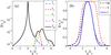 |
Fig. A.1 Illustration of the distribution function model. a) The total and the four components of the distribution function shown by the blue curves in Figs. 4f and i. b) The M(v) and T(v) factors of Eq. (3) and the product f(v) = M(v)T(v) for the rising slope of the tail in Figs. 4d and g. The velocity scale is normalised to |
Panel b) of Fig. A.1 shows one of the components of the distribution represented by the blue curves in Fig. 4d and g. This component is used to fit the model distribution to the data for the rising edge of the tail, peaking at vχ = 17 km s-1 in Fig. 4d. The parameters of the simple pole expansion are shown in Table A.2.
The centre of the T(v) function (dashed red curve) is displaced 0.3cs from the centre of the M(v) function (dashed black curve). This makes the rising slope of the product f(v) = M(v)T(v) (solid blue curve) steeper than the falling slope.
The supplementary material includes computer code to compute dispersion relations and input files for all distribution functions shown in Fig. 4.
All Tables
All Figures
|
Fig. 1 Illustration of particle motion at 67P/Churyumov-Gerasimenko, showing outgassing of neutral water molecules, the beginning of the H2O+ trajectories, and deflection of solar wind ions. During the observations reported in this paper the position of the spacecraft was 28 km from the comet, which was 2.5 AU from the Sun. Schematic of solar wind deflection adapted from Behar et al. (2016a). Photo of nucleus and spacecraft: ESA – European Space Agency. |
| In the text | |
|
Fig. 2 Geometry of the observations. Panels a)–c) show the viewing directions, that is, the centres of the fields of view, for the RPC-ICA instrument projected onto the plane containing the comet to spacecraft direction and the CSEQ x direction for times 08:00, 16:24, and 20:46 in panels a)−c), respectively. The nucleus of the comet is located at the origin of the coordinate system. For the same times, panels d)–f) show the orientation of the spacecraft and the ROSINA COPS instrument with respect to the gas flow from the nucleus, which is shown by the black arrows. |
| In the text | |
|
Fig. 3 Overview of the observations by instruments on board the Rosetta spacecraft on 20 January 2015. a) Ion energy spectrum measured by RPC-ICA. The colour coded quantity is the differential particle flux summed over all viewing directions. The energy scale has been adjusted for Vsc and Voffset. b) Differential particle flux of hot water ions (9 eV ≲ E ≲ 23 eV when E is adjusted for offset and spacecraft potential) for the different sectors of the RPC-ICA instrument. c) Electron temperature observed by RPC-LAP. d) Magnitude of the magnetic flux density B seen by RPC-MAG. e) Neutral gas density measured by ROSINA-COPS. f) Angles between the coordinate axes of the spacecraft frame of reference and the direction to the nucleus of the comet. g) Power Spectral density of the current to Langmuir probe 1 in the frequency range 200 Hz <f ≤ 1450 Hz. h) Power Spectral density of the current to Langmuir probe 2 for 200 Hz <f ≤ 1450 Hz. Periods when the ROSINA-COPS measurements were affected by the spacecraft pointing are marked in grey at the bottom of panel e) and the top of panel f). The spikes in the neutral density at 03:54, 14:00, and 23:31 (shown in grey in panel e)) are due to wheel off-loading manoeuvres. The RPC-ICA instrument (panels a) and b)) was off during these manoeuvres. |
| In the text | |
|
Fig. 4 Water ion distribution functions observed at 08:00 (left column), 16:24 (mid column), and 20:46 (right column) on 20 January 2015. Panels a)–c) show the two-dimensional projection of the distribution function on a plane in velocity space. Panels d)–f) show the one-dimensional projection of the distribution functions on the horizontal axis of panels a)–c). Panels g)–i) show the same one-dimensional projection on a logarithmic vertical scale. The black curves show the data. The red, blue, and green curves show three different functions used as fits to the data. Corrections for the instrument offset and spacecraft potential have been applied. Densities and temperatures for the model curves are shown in Table 1. |
| In the text | |
|
Fig. 5 Comparison of densities derived from RPC-ICA measurements to those from RPC-LAP and RPC-MIP. The blue and red lines show the minimum and maximum RPC-MIP plasma density estimates, respectively. Estimates based on RPC-LAP data are marked “×”. The two sets of estimates derived from RPC-ICA data assuming the ion distribution to be isotropic for vi ≲ 7 km s-1 and vi ≲ 12 km s-1 are marked “∗” and “°”, respectively. The data sets were recorded on 19 January 2015. |
| In the text | |
|
Fig. 6 Panels a), c), and e): power spectral densities of the currents to the Langmuir probes at 08:00, 16:24, and 20:46 on 20 January 2015. The red lines show probe 1 and the black lines probe 2. The dashed lines show lower frequency resolution, where data points taken while the RPC-MIP instrument was running have been removed. The error bars show the 95% confidence intervals for the solid curves in blue and the dashed curves in green. Panels b), d), and f) power spectral densities divided by ω2. |
| In the text | |
|
Fig. 7 Dispersion relations at 08:00 on 20 January 2015. a) Distribution functions for cometary water ions (solid blue curve) and solar wind protons (dash-dotted orange curve) and alpha particles (dashed black curve). b) Real part of ω as a function of wave number. c) The imaginary part of ω as a function of wave number. In this case γ> 0 for all three curves, which means that these modes are damped. The blue curves represent the same mode as the blue curves in Fig. 8. |
| In the text | |
|
Fig. 8 Dispersion relations at 08:00 on 20 January 2015. a) Real part of ω as a function of wave number. b) The imaginary part of ω as a function of wave number. For growing modes γ< 0 and for damped modes γ> 0. The red, blue, and green curves correspond to the distribution functions shown in Figs. 4d and g by the red, blue, and green curves, respectively. |
| In the text | |
|
Fig. 9 Dispersion relations at 16:24 on 20 January 2015. a) Real part of ω as a function of wave number. b) The imaginary part of ω as a function of wave number. For growing modes γ < 0 and for damped modes γ > 0. The red, blue, and green curves correspond to the distribution functions shown in Fig. 4e and h by the red, blue and green curves, respectively. |
| In the text | |
|
Fig. 10 Dispersion relations at 20:46 on 20 January 2015. a) Real part of ω as a function of wave number. b) The imaginary part of ω as a function of wave number. For growing modes γ < 0 and for damped modes γ > 0. The red, blue, and green curves correspond to the distribution functions shown in Figs. 4f and i by the red, blue, and green curves, respectively. |
| In the text | |
|
Fig. A.1 Illustration of the distribution function model. a) The total and the four components of the distribution function shown by the blue curves in Figs. 4f and i. b) The M(v) and T(v) factors of Eq. (3) and the product f(v) = M(v)T(v) for the rising slope of the tail in Figs. 4d and g. The velocity scale is normalised to |
| In the text | |
Current usage metrics show cumulative count of Article Views (full-text article views including HTML views, PDF and ePub downloads, according to the available data) and Abstracts Views on Vision4Press platform.
Data correspond to usage on the plateform after 2015. The current usage metrics is available 48-96 hours after online publication and is updated daily on week days.
Initial download of the metrics may take a while.