| Issue |
A&A
Volume 600, April 2017
|
|
|---|---|---|
| Article Number | A59 | |
| Number of page(s) | 15 | |
| Section | Celestial mechanics and astrometry | |
| DOI | https://doi.org/10.1051/0004-6361/201629679 | |
| Published online | 30 March 2017 | |
A new insight into the Galactic potential: A simple secular model for the evolution of binary systems in the solar neighbourhood
1 Grupo de Ciencias Planetarias, Complejo Astronómico El Leoncito, UNLP, UNC, UNSJ, CONICET, Av. España 1512 sur, J5402DSP San Juan, Argentina
e-mail: This email address is being protected from spambots. You need JavaScript enabled to view it.
2 Universidad Nacional de San Juan, J. I. de la Roza 590 oeste, 5400 Rivadavia, San Juan, Argentina
Received: 9 September 2016
Accepted: 4 November 2016
Abstract
Context. Among the main effects that the Milky Way exerts in binary systems, the Galactic tide is the only one that is not probabilistic and can be deduced from a potential. Therefore, it is possible to perform an analysis of the global structure of the phase space of binary systems in the solar neighbourhood using the Galactic potential.
Aims. The aim of this work is to obtain a simple model to study the collisionless dynamical evolution of generic wide binaries systems in the solar neighbourhood.
Methods. Through an averaging process, we reduced the three-dimensional potential of the Galaxy to a secular one-degree of freedom model. The accuracy of this model was tested by comparing its predictions with numerical simulations of the exact equations of motion of a two-body problem disturbed by the Galaxy.
Results. Using the one-degree of freedom model, we developed a detailed dynamical study, finding that the secular Galactic tide period changes as a function of the separation of the pair, which also gives a dynamical explanation for the arbitrary classification between “wide” and “tight” binaries. Moreover, the secular phase space for a generic gravitationally bound pair is similar to the dynamical structure of a Lidov-Kozai resonance, but surprisingly this structure is independent of the masses and semimajor axis of the binary system. Thus, the Galactic potential is able to excite the initially circular orbit of binary systems to high values of eccentricity, which has important implications for studies of binary star systems (with and without exoplanets), comets, and Oort cloud objects.
Key words: galaxies: kinematics and dynamics / binaries: general / solar neighborhood / methods: analytical / methods: numerical / planets and satellites: dynamical evolution and stability
© ESO, 2017
1. Introduction
The binary systems in the solar neighbourhood are commonly associated with gravitationally bounded stars. However, the Sun and a comet or an Oort cloud object can also be considered a binary system in the framework of a restricted two-body problem. For any of these pairs, their orbits mainly change by the influence of Galactic tides and encounters with close passing stars and molecular clouds (Brunini 1995; Eggers & Woolfson 1996; Levison & Dones 2001; Fouchard et al. 2006; Jiang & Tremaine 2010; Kaib et al. 2011, 2013).
The effect exerted by the Milky Way on a binary system depends on its orbit, since its semimajor axis (a) regulates the influence of the Galactic environment. Binary systems with a large separation are weakly bound by self-gravity, and therefore they are the most disturbed by the Galaxy (Heggie 1975; Bahcall et al. 1985; Jiang & Tremaine 2010). These configurations with a> 1000 au are called “wide binaries” (Roell et al. 2012) and a system with smaller semimajor axis is considered a “tight or close” binary. This limit (~1000 au) is defined empirically, but there is not an analytic deduction that supports it.
In the solar neighbourhood, our Galaxy disturbs a binary system with two main effects: first, the tidal field of the Milky Way and, second, the gravitational perturbation from passing stars or other perturbers (e.g. molecular clouds). However, while the Galactic tidal field is derived from an analytical potential, the effects of encounters caused by passing stars (or other object) correspond to a stochastic perturbation on the pair.
Therefore, because of the random influence of the Milky Way in wide pairs, almost all the works carried out in this area are statistical studies (Brunini 1995; Eggers & Woolfson 1996; Levison & Dones 2001; Fouchard et al. 2006; Jiang & Tremaine 2010). However, despite the dynamic importance of a theoretical analysis about the effect of the Galactic tide on a binary system, it is difficult to find these types of studies in the literature.
Heisler & Tremaine (1986) performed an analytical study of the Galactic potential for the restricted two-body problem (i.e. Sun-comet), but they focused on the lost rate of minor bodies due to the Galactic tide and stellar encounters. We have not found a specific study about the dynamic portrait of the secular phase space of a binary system disturbed by the gravitational potential of the Milky Way.
The importance of a detailed dynamical study about these systems relies on the possibility of simplifying the Hamiltonian. Such a mathematical procedure allows us to reduce the equations of motion, with the consequent low computational cost, despite the diversity of systems and initial configurations that can be analysed.
The aims of the present work are twofold: first, to obtain a simple model for the secular evolution of a pair of objects that are gravitationally bound and located in the solar neighbourhood, and second, through that model, to perform a detailed study of the effects of the Galactic gravitational potential in generic binary systems (i.e. star-star, Sun-comet, etc.).
In Sect. 2 we deduce the model that has one-degree of freedom. In Sect. 3 the model is used to find the position of the equilibrium points of the Hamiltonian. In Sect. 4 a detailed analysis of the phase space of a binary system is presented. An application of the model is in Sect. 5. Conclusions close the paper in Sect. 6.
2. The model for the Galactic potential
We allow m1 and m2 to be the masses of the components of a binary system (i.e. star-star, star-planet, Sun-comet, etc.), which are negligible compared with the mass of the Galaxy. The motion of such a binary system in the Galaxy can be described by the use of the Hill approximation (Heggie 2001; Binney & Tremaine 2008). We consider a non-inertial Cartesian astrocentric coordinate system (x,y,z) with origin in the main body (m1). This system is at a distance Rg from the Galactic centre, and corotates with the Galaxy. The z-axis is perpendicular to the Galactic plane and points towards the south Galactic pole, the y-axis points in the direction of Galactic rotation, and the x-axis points radially outwards from the Galactic centre.
Then, assuming a symmetric potential on the plane z = 0, the Galactic tide disturbs the binary system according to the Hamiltonian, 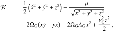 (1)where
  ,
,  is the gravity constant and x, y, z, ẋ, ẏ, ż are the astrocentric components of position and velocity of the secondary body m2 around m1. Moreover, ΩG, AG, and νG are the angular speed of the Galaxy, Oort constant, and frequency for small oscillations in z, respectively. For Rg = 8 kpc (i.e. approximately the distance from the Galactic centre to the Sun) their values are (Jiang & Tremaine 2010)
 ![Mathematical equation: \begin{equation} \begin{array}{ccl} \Omega_{\rm G} &\cong& 3.017 \times 10^{-8} \, {\rm yr}^{-1}\, \rm{,} \\[1mm] A_{\rm G} &\cong& 1.513 \times 10^{-8} \, {\rm yr}^{-1} \rm{,} \\[1mm] \nu_{\rm G} &\cong& 7.258 \times 10^{-8} \, {\rm yr}^{-1} \rm{.} \label{eq2} \end{array} \end{equation}](/articles/aa/full_html/2017/04/aa29679-16/aa29679-16-eq22.png) (2)
(2)
The equations of motion for this Hamiltonian are (see Jiang & Tremaine 2010) ![Mathematical equation: \begin{equation} \begin{array}{cclccl} \dot{x} &=& \dfrac{\partial \mathcal{K}}{\partial \dot{x}} , & \ddot{x} &=& -\dfrac{\partial \mathcal{K}}{\partial x} \rm{,}\\[2mm] \dot{y} &=& \dfrac{\partial \mathcal{K}}{\partial \dot{y}} , & \ddot{y} &=& -\dfrac{\partial \mathcal{K}}{\partial y} \rm{,} \\[2mm] \dot{z} &=& \dfrac{\partial \mathcal{K}}{\partial \dot{z}} , & \ddot{z} &=& -\dfrac{\partial \mathcal{K}}{\partial z} \cdot \label{eq3} \end{array} \end{equation}](/articles/aa/full_html/2017/04/aa29679-16/aa29679-16-eq23.png) (3)In dynamical studies it is convenient to work with orbital elements instead of Cartesian coordinates. Once again, we place the centre of the coordinate system in m1, and then the orbital elements correspond to the astrocentric orbit of m2 around m1. We define the orbital elements as follows: the size and form of the orbit are defined by the semimajor axis a and the eccentricity e, respectively. The mean anomaly M indicates the position of m2 in the orbit. The reference plane is the mid-plane of the Galaxy, and its intersection with the orbital plane of m2 defines the position of the ascending node. The direction radially outwards from the Galactic centre (i.e. x−axis) is taken as reference to define the angular position of the ascending node Ω, where the angle is measured in anti-clockwise sense (i.e. towards the positive y-axis). The inclination I is defined with respect to the reference plane, and the argument of pericentre ω is measured from the ascending node in an anti-clockwise sense. For these astrocentric orbital elements, we can define the Hamiltonian as
(3)In dynamical studies it is convenient to work with orbital elements instead of Cartesian coordinates. Once again, we place the centre of the coordinate system in m1, and then the orbital elements correspond to the astrocentric orbit of m2 around m1. We define the orbital elements as follows: the size and form of the orbit are defined by the semimajor axis a and the eccentricity e, respectively. The mean anomaly M indicates the position of m2 in the orbit. The reference plane is the mid-plane of the Galaxy, and its intersection with the orbital plane of m2 defines the position of the ascending node. The direction radially outwards from the Galactic centre (i.e. x−axis) is taken as reference to define the angular position of the ascending node Ω, where the angle is measured in anti-clockwise sense (i.e. towards the positive y-axis). The inclination I is defined with respect to the reference plane, and the argument of pericentre ω is measured from the ascending node in an anti-clockwise sense. For these astrocentric orbital elements, we can define the Hamiltonian as 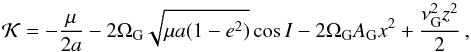 (4)where
 ![Mathematical equation: \begin{eqnarray} x &=& a \bigg\{ \cos \Omega \left[ (\cos E - e) \cos \omega - \sqrt{1-e^2} \sin E \sin \omega\right]\nonumber \\ &&- \cos I \sin \Omega \left[ (\cos E - e) \sin \omega + \sqrt{1-e^2} \sin E \cos \omega \right] \bigg\} \, \rm{,} \nonumber\\ z &=& a \sin I \left[ (\cos E - e) \sin \omega + \sqrt{1-e^2} \sin E \cos \omega \right] \rm{,} \label{eq5} \end{eqnarray}](/articles/aa/full_html/2017/04/aa29679-16/aa29679-16-eq31.png) (5)and E is the eccentric anomaly, which is an implicit function of the mean anomaly (M = E−esinE).
(5)and E is the eccentric anomaly, which is an implicit function of the mean anomaly (M = E−esinE).
The first term in Eq. (4) corresponds to the two-body contribution,  . The second term in Eq. (4) is the z component of the angular momentum multiplied by the angular speed of the Galaxy (ΩG) and it is included because we are working in a non-inertial frame. The influence of this term (
 ) is small compared with the two-body term . Finally, the last two terms correspond to the tidal perturbation of the Galaxy, which are still smaller than the previous terms, so both are considered a perturbation called
  . Then, we can schematically write the Hamiltonian as a disturbed two-body problem,
 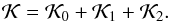 (6)Considering the distant-tide approximation (Jiang & Tremaine 2010), it is possible to write the effects of the Galactic tidal field (i.e. ) about Rg = 8 kpc using a Taylor series expansion. We truncate the series expansion at second order in
  , as in many other works (Heisler & Tremaine 1986; Jiang & Tremaine 2010; Kaib et al. 2013). Although it is possible to consider higher orders of the series, their effects are negligible for the range of distance (r) considered in this paper (Sect. 2.2) and also for larger separations between the pair Jiang & Tremaine (2010).
However, the orbital elements are not canonical variables, which makes the application of the canonical perturbation theory difficult (Morbidelli 2002; Ferraz-Mello 2007), despite the complex equations of variation of the orbital elements. Then, a better choice is to work with the canonical action-angles variables of Delaunay associated with the orbital elements defined above written as 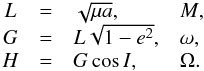 (7)In these variables the Hamiltonian is defined as
 ![Mathematical equation: \begin{equation} \begin{array}{ccl} \mathcal{K}_0 &=& - \frac{1}{2}\mu^2 L^{-2} \rm{,} \\[2mm] \mathcal{K}_1 &=& - 2 \Omega_{\rm G} H \rm{,} \\ \mathcal{K}_2 &=& - 2 \Omega_{\rm G} A_{\rm G} x^2 + \dfrac{1}{2} \nu_{\rm G}^2 z^2 \rm{,} \label{eq8} \end{array} \end{equation}](/articles/aa/full_html/2017/04/aa29679-16/aa29679-16-eq42.png) (8)where
(8)where ![Mathematical equation: \begin{equation} \begin{array}{ccl} x & = & \dfrac{L^2}{\mu} \Bigg [ \cos E \left( \cos \omega - \dfrac{H}{G} \sin \omega \sin \Omega \right) \\[2mm] & &- \dfrac{G}{L} \sin E \left( \sin \omega \cos \Omega + \dfrac{H}{G} \cos \omega \sin \Omega \right) \\[2mm] & &+ \sqrt{1- \left( \dfrac{G}{L} \right)^2} \left(\dfrac{H}{G} \sin \omega \sin \Omega - \cos \omega \cos \Omega \right) \Bigg] \rm{,} \\[2mm] z & = & \dfrac{L^2}{\mu} \sqrt{1- \left( \dfrac{H}{G} \right)^2} \Bigg [ \cos E \sin \omega \\[2mm] && + \dfrac{G}{L} \sin E \cos \omega - \sqrt{1- \left( \dfrac{G}{L} \right)^2} \sin \omega \Bigg] \rm{,} \label{eq9} \end{array} \end{equation}](/articles/aa/full_html/2017/04/aa29679-16/aa29679-16-eq43.png) (9)and with these variables, the equations of variation of the orbital elements are the following Delaunay equations:
(9)and with these variables, the equations of variation of the orbital elements are the following Delaunay equations: ![Mathematical equation: \begin{equation} \begin{array}{cclccl} \dot{M} &=& \dfrac{\partial \mathcal{K}}{\partial L} , & \dot{L} &=& -\dfrac{\partial \mathcal{K}}{\partial M} \, \rm{,} \\[2mm] \dot{\omega} &=& \dfrac{\partial \mathcal{K}}{\partial G} , & \dot{G} &=& -\dfrac{\partial \mathcal{K}}{\partial \omega} \rm{,} \\[2mm] \dot{\Omega} &=& \dfrac{\partial \mathcal{K}}{\partial H} , & \dot{H} &=& -\dfrac{\partial \mathcal{K}}{\partial \Omega} \cdot \label{eq10} \end{array} \end{equation}](/articles/aa/full_html/2017/04/aa29679-16/aa29679-16-eq44.png) (10)For the objectives of this paper, it is convenient to write the Eq. (9) as
(10)For the objectives of this paper, it is convenient to write the Eq. (9) as ![Mathematical equation: \begin{equation} \begin{array}{ccl} x & = & a x_1 \, \\[1mm] z & = & a z_1 \rm{,} \label{eq9b} \end{array} \end{equation}](/articles/aa/full_html/2017/04/aa29679-16/aa29679-16-eq45.png) (11)where x1 and z1 are functions of the orbital elements e, I, M, ω, and Ω with their range of values between –1 and 1. Moreover, the derivative of these functions with respect to the action variables L, G, and H can also be written in a simplified form as
(11)where x1 and z1 are functions of the orbital elements e, I, M, ω, and Ω with their range of values between –1 and 1. Moreover, the derivative of these functions with respect to the action variables L, G, and H can also be written in a simplified form as![Mathematical equation: \begin{equation} \begin{array}{ccl} \dfrac{\partial x}{\partial \chi} & = & \sqrt{\dfrac{a}{\mu}} x_\chi \\[4mm] \dfrac{\partial z}{\partial \chi} & = & \sqrt{\dfrac{a}{\mu}} z_\chi \rm{,} \label{eq9c} \end{array} \end{equation}](/articles/aa/full_html/2017/04/aa29679-16/aa29679-16-eq52.png) (12)with χ representing any of the action variables. The functions xχ and zχ are dependent of the orbital elements e, I, M, ω, and Ω, and they are bounded in the range ∈ (–1, 1).
(12)with χ representing any of the action variables. The functions xχ and zχ are dependent of the orbital elements e, I, M, ω, and Ω, and they are bounded in the range ∈ (–1, 1).
Finally, the limit for the disturbed two-body problem depends on the semimajor axis, since for small values of a the perturbations of the Galaxy ( and ) are too small. However, with the increase of the semimajor axis such approximation is no longer valid because of the increase of the disturbing terms (i.e. we leave the regime of a disturbed two-body problem).
2.1. The one-degree of freedom model
The Hamiltonian (6) can be written as  (13)with,
 ![Mathematical equation: \begin{equation} \begin{array}{ccl} \mathcal{K}_{g0} &=& - \dfrac{\mu^2}{2 L^{2}} - 2 \Omega_{\rm G} H \rm{,} \\[3mm] \epsilon &=& \left( \dfrac{a}{r_J} \right) ^3 \rm{,} \\[3mm] \mathcal{K}_{g1} &=& - \dfrac{\mu}{2 \, a^3} x^2 + \dfrac{\beta \, \mu}{4 \, a^3} z^2 \rm{,} \label{eq6c} \end{array} \end{equation}](/articles/aa/full_html/2017/04/aa29679-16/aa29679-16-eq58.png) (14)where
(14)where  (15)is a constant and
  (16)is the radius of Jacobi of a binary system in the tidal field of the Galaxy (Jiang & Tremaine 2010). Considering a three-body system composed by the binary system and the Galaxy, the tidal radius rJ is the position of the stationary Lagrange points L1, which defines the Roche lobe of the binary. Here,
  is the integrable approximation,
  the disturbing function or perturbation. and ϵ a small parameter. Thus, we can represent the Hamiltonian (6) as the Hamiltonian of a quasi-integrable system (Morbidelli 2002; Ferraz-Mello 2007). Moreover, the quasi-integrable Hamiltonian (13) can be written in the simplified form,
  (17)where
 ![Mathematical equation: \begin{equation} \begin{array}{ccl} f_{\rm o} &=& \dfrac{\partial \mathcal{K}_0}{\partial L} = n \rm{,} \\[3mm] f_{\rm n} &=& \dfrac{\partial \mathcal{K}_0}{\partial H} = -2 \Omega_{\rm G} \, \rm{} \label{eq6f} \end{array} \end{equation}](/articles/aa/full_html/2017/04/aa29679-16/aa29679-16-eq67.png) (18)are the frequencies of the integrable approximation and n the mean motion of the binary system. Therefore, we can perform a first-order averaging of the Hamiltonian over the fast angles M and Ω. This averaging is performed by the Hori method at first order (Morbidelli 2002; Ferraz-Mello 2007), which takes advantage of the Lie series and is similar to the transformation of Von Zeipel-Brouwer (Brouwer & Clemence 1961; Naoz et al. 2013).
(18)are the frequencies of the integrable approximation and n the mean motion of the binary system. Therefore, we can perform a first-order averaging of the Hamiltonian over the fast angles M and Ω. This averaging is performed by the Hori method at first order (Morbidelli 2002; Ferraz-Mello 2007), which takes advantage of the Lie series and is similar to the transformation of Von Zeipel-Brouwer (Brouwer & Clemence 1961; Naoz et al. 2013).
The averaged Hamiltonian can be written as  (19)where
  has the same functional form that , and
  define the homologic equation,
  (20)with χg as the generating function.
In order to solve the homologic equation we take advantage of the Hamiltonian (6), which is periodic in the angles M and Ω, the disturbing function can thereby be expanded in Fourier series,  (21)where q = (M,Ω,ω) and n is an integer vector. Then, for a similar expansion of the homologic equation, the averaged disturbing function is simply
  . The corresponding coefficient c0 of the Fourier expansion is
  (22)or using the implicit relation M = E−e sinE and its differential form dM = 1−e cosE dE, we can write
  (23)For more details about the averaging process, see Chap. 2 of Morbidelli (2002).
Then, the averaging disturbing function is defined as ![Mathematical equation: \begin{equation} \begin{array}{ccl} \mathcal{K}_{g1}^* & = & \dfrac{\mu^2}{4\,{L^*}^2} \bigg\lbrace \dfrac{\alpha}{{G^*}^2} \big[ \left(2{L^*}^2-{G^*}^2\right) \left({G^*}^2-{H^*}^2\right) \\[3mm] & & - \left({L^*}^2-{G^*}^2\right) \left({G^*}^2-{H^*}^2\right) \cos{2\omega^*} \big] \\[3mm] && - \left(2{L^*}^2-{G^*}^2\right) \bigg\rbrace \rm{,} \end{array} \label{eq61} \end{equation}](/articles/aa/full_html/2017/04/aa29679-16/aa29679-16-eq83.png) (24)
(24)
with α = 0.5(1 + β). In terms of astrocentric orbital elements, the mean-mean or averaged disturbed function can be expressed as ![Mathematical equation: \begin{equation} \mathcal{K}_{g1}^* \, = \, \dfrac{\mu}{4\,{a^*}} \left[ \alpha (\sin{{I^*}})^2 \left(1+{e^*}^2 - {e^*}^2 \cos{2\omega^*}\right) - \left(1+{e^*}^2\right) \right] \rm{,} \label{eq61b} \end{equation}](/articles/aa/full_html/2017/04/aa29679-16/aa29679-16-eq85.png) (25)where a∗, e∗, I∗, ω∗ are the mean-mean orbital elements averaged in the fast angles M and Ω.
(25)where a∗, e∗, I∗, ω∗ are the mean-mean orbital elements averaged in the fast angles M and Ω.
From the averaging process we obtain new canonical variables (L∗, G∗, H∗, M∗, ω∗, Ω∗) such that the transformed Hamiltonian is K∗ =  (G∗, ω∗; L∗, H∗) and M∗ and Ω∗ are cyclic. The associated momenta L∗ and H∗ are then new constants of motion, and the system is reduced to a model with one-degree of freedom for the canonical variables (G∗, ω∗). Thus, the mean-mean Hamiltonian, which defines our one-degree of freedom model, is
 (26)with
 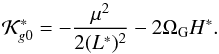 (27)Owing to the conservation of \begin{lxirformule}$H^*$\end{lxirformule} (
 ), there is a coupling between the eccentricity and inclination, and thereby the dynamical behaviour of the system seems to be similar to the Lidov-Kozai resonance (Lidov 1961; Kozai 1962; Naoz 2016).
2.2. Scope of the approximation
The scope of our quasi-integrable Hamiltonian (6) is defined by the weight of the disturbing function. The second term of the right part in Eq. (6) must be a small perturbation over the integrable Hamiltonian .
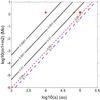 |
Fig. 1 Level curves of constant ϵ in the plane (a, m1 + m2). The dotted red line indicates the limit for the integrable approximation. The approximation fails for the binary systems below the dashed blue line. The red symbols (cross, triangle, and circle) represent the position of three binary systems (see Sect. 2.5). |
The integrable Hamiltonian has two terms and working algebraically we obtain 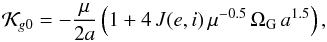 (28)where J is a function with values in the range ∈ (–1, 1). The functional form of the second term in the parenthesis of the right side in Eq. (28) can be approximately by its dependence on a because the range of values of the parameter μ is smaller than the range of the semimajor axis. So, the second term in the parenthesis becomes comparable to 1 for a ~ 105 au. In this way we can approximate
  . On the other hand, the perturbation can be written using the simplified forms (11) and (12),
 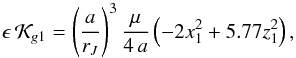 (29)and then,
  . Therefore, the integrable Hamiltonian and the disturbing function are comparable terms, being
  who defines the weight of the perturbation. The limit for the disturbing regime is difficult to define, but we can consider ϵ ~ 0.05 as the upper limit for the quasi-integrable approximation.
However, the small parameter only depends on the semimajor axes and the masses  (30)Thus, the scope of the one-degree of freedom model is defined by two parameters. Figure 1 shows level curves of ϵ in the plane (a, m1 + m2), with the approximated upper limit (ϵ ~ 0.05) shown with a dotted red line. The binary systems below the dashed blue curve cannot be approximated by the model, but these are very separated pairs of small masses. Finally. we can quickly estimate the limit of the integrable approximation for any binary system from the graph.
2.3. Numerical approximation of the one-degree of freedom model
The weak effect of the Galactic perturbation for the case ϵ< 0.05 can also be deduced from the motion equation of the complete three-degree of freedom model.
The temporal evolution of the mean anomaly (Eq. (10)) is defined as  (31)
(31)
The second term in the right side of the Eq. (31) is zero since it is independent of L, the first term is the mean motion of the astrocentric orbit of m2 around m1, and the last term is the perturbation of the Galaxy, (32)where
  (33)
(33)
which can be written using a simplified form (Eqs. (11) and (12)), i.e. 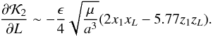 (34)Because we are considering ϵ< 0.05 the second term in the right part of Eq. (32) is smaller than the mean motion of the binary system. Therefore, the perturbation of the Galaxy is small enough to use the approximation M ~ nt + τn (τn is an arbitrary constant). So, M circulates with a frequency n, and the semimajor axis has an almost constant evolution with a small amplitude.
The precession frequency of the ascending node is defined as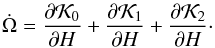 (35)In this equation the first term of the right part is zero since
  is independent of H, the second term is the motion of the binary system around the Galaxy, and the last term corresponds to the tidal perturbation of the Galaxy,
 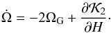 (36)where
 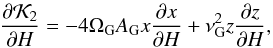 (37)which can be written using a simplified form (Eqs. (11) and (12)), i.e.
 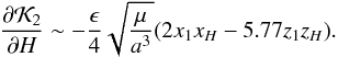 (38)In this case, for ϵ< 0.05 the second term in the right side of Eq. (36) is smaller than the angular velocity of the binary system around the Galaxy (i.e. ΩG).
Then, since the perturbation of the Galaxy is small we can write Ω ~ 2ΩGt + τo (τo is an arbitrary constant), which corresponds to a circulation of the angle Ω with frequency 2ΩG, the action H has small variations and can be considered almost constant. The circulation of Ω is related to the orbital period of the binary system around the centre of the Galaxy.
The frequency of the argument of pericentre is defined as 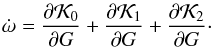 (39)The first and second terms on the right side are independent of G∗ and then are equal to zero. The last term, which is small, defines the tidal perturbation of the Galaxy on the binary system. So, the frequency is defined by
 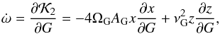 (40)which can be simplified with the approximations (11) and (12),
 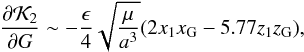 (41)which define the secular evolution of the binary system.
Thus, for ϵ< 0.05 the equations of motion for the original three-degree of freedom model can be approximated by ![Mathematical equation: \begin{equation} \begin{array}{lclccl} \dot{M} &\sim& n , & \dot{L} &\sim& 0 \rm{,} \\[2mm] \dot{\omega} &=& \dfrac{\partial \mathcal{K}_2}{\partial G} , & \dot{G} &=& -\dfrac{\partial \mathcal{K}_2}{\partial \omega} \rm{,} \\[2mm] \dot{\Omega} &\sim& -2 \Omega_{\rm G} , & \dot{H} &\sim& 0 \rm{.} \label{eq19} \end{array} \end{equation}](/articles/aa/full_html/2017/04/aa29679-16/aa29679-16-eq129.png) (42)In this approximation L and H are almost constants with small variations, and the angles M and Ω circulate with an osculating period Tn ~ 2π/n and a Galactic rotational period To ~ π/ Ωg ~ 108 yr, respectively. The latter defines the small precession of the ascending node, which is related to the circulation of the system around the Galaxy. Hence, the tidal secular evolution has a dynamical behaviour that can be approximated by a system of one-degree of freedom and is defined by the pair action-angle variables G and ω. The almost constant value of H implies a dynamical behaviour of e and I that is similar to the dynamic of the Lidov-Kozai resonance, such as we deduce from the averaging process.
(42)In this approximation L and H are almost constants with small variations, and the angles M and Ω circulate with an osculating period Tn ~ 2π/n and a Galactic rotational period To ~ π/ Ωg ~ 108 yr, respectively. The latter defines the small precession of the ascending node, which is related to the circulation of the system around the Galaxy. Hence, the tidal secular evolution has a dynamical behaviour that can be approximated by a system of one-degree of freedom and is defined by the pair action-angle variables G and ω. The almost constant value of H implies a dynamical behaviour of e and I that is similar to the dynamic of the Lidov-Kozai resonance, such as we deduce from the averaging process.
2.4. Frequency analysis
From the three natural frequencies involved in the problem we can perform a brief comparative analysis between them, such as that carried out by Antognini (2015). A frequency analysis (Michtchenko et al. 2002) is very important because this allows us to predict the interaction between the natural frequencies of the system, which can act as a source of chaos (i.e. commensurable periods). Our previous deduction of the angular frequencies allows us to define the secular (fs), node-precession (fn), and osculating (fo) frequencies as 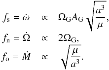 (43)Then, the ratio between these frequencies are
 ![Mathematical equation: \begin{equation} \begin{array}{ccl} f_{\rm o}/f_{\rm s} &\sim& \dfrac{4}{\epsilon } \rm{,} \\[2mm] f_{\rm n}/f_{\rm s} &\sim& 4 \sqrt{\dfrac{\Omega_{\rm G}}{ A_{\rm G} \epsilon }} \rm{,} \\[2mm] f_{\rm o}/f_{\rm n} &\sim& \sqrt{\dfrac{A_{\rm G}}{ \Omega_{\rm G} \epsilon }} \cdot \label{eq19rx} \end{array} \end{equation}](/articles/aa/full_html/2017/04/aa29679-16/aa29679-16-eq137.png) (44)Figure 2 shows the ratio between the frequencies for the same range of masses and semimajor axis of Fig. 1. The relation between the high frequencies and the secular frequency are indicated with a dashed black line for fo/fs, and dotted blue line for fn/fs. For simplicity, we only plot levels 1 and 10 because the commensurable region is restricted to binary systems with particular characteristics. The ratio fo/fn is plotted with a red line and we show the levels 1, 2, 5, and 10. For the high frequencies, the commensurability (fo/fn ≤ 5) achieves a greater region in the plane (a, m1 + m2).
(44)Figure 2 shows the ratio between the frequencies for the same range of masses and semimajor axis of Fig. 1. The relation between the high frequencies and the secular frequency are indicated with a dashed black line for fo/fs, and dotted blue line for fn/fs. For simplicity, we only plot levels 1 and 10 because the commensurable region is restricted to binary systems with particular characteristics. The ratio fo/fn is plotted with a red line and we show the levels 1, 2, 5, and 10. For the high frequencies, the commensurability (fo/fn ≤ 5) achieves a greater region in the plane (a, m1 + m2).
 |
Fig. 2 Level curves of the ratio between the frequencies: fo/fs (dashed black line), fn/fs (dotted blue line) and fo/fn (red line). For the comparison with the secular frequency we plot the ratio 1 and 10. For the comparison between the fast frequencies (fo/fn) we plot the levels 1, 2, 5 and 10. The red symbols (cross, triangle and circle) represent the position of three binary systems (see Sect. 2.5). |
For binary systems with a < 3 × 10⁶ au (~1.5 pc), the problem of the interaction of the secular frequency with the other periods is restricted to small masses. For binary systems with m1 + m2 > 0.1M⊙, fo and fn are commensurate for a > 60 000 au. Then, the application of the secular one-degree of freedom model is accurate for binary systems with fo/fn ≥ 5. The scope of the model (Sect. 2.2) is close to the start of the non-secular region.
Finally, the approximated secular frequency for binary systems with a < 1000 au and m1 + m2 < 10 M⊙ (Eq. (43)) has an associated period of hundred of Gyr. Such a period is an order of magnitude greater than the age of the universe (i.e. ~13 Gyr). This gives a theoretical explanation for the empirical limit of 1000 au between tight and wide binary systems .
 |
Fig. 3 Time evolution of the action variables of Delaunay L (top panel), H (middle panel) and G (bottom panel) for our standard system. The small variations of L and H and the circulation of M and Ω (Fig. 4) confirm the proposed approximation. |
 |
Fig. 4 Time evolution of the angular variables of Delaunay M (top panel), Ω (middle panel) and ω (bottom panel) for our standard system. The small variations of L and H (Fig. 3) and the circulation of M and Ω confirm the approximation proposed. |
2.5. Testing the one-degree of freedom model: an application example
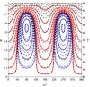 |
Fig. 5 Comparison between the predictions of our model (dashed black line) and numerical simulations (red and blue lines) in the plane (ω∗,e∗), for the family of solutions of the standard system. |
In order to show the use of the model we use a binary system with masses m1 = 1.0M⊙ and m2 = 0.3M⊙ as an example. The secondary star is moving around the main star in an initial configuration named “standard system”, where the initial parameters are a0 = 10 000 au (L0 = 716.4 au2/yr), e0 = 0.2 (G0 = 702 au2/yr), I0 = 53° (H0 = 421.86 au2/yr), and ω0 = 90°. The other two angles are equal to zero. Figures 3 and 4 show the temporal evolution of the action and angle variables of Delaunay, respectively. In these figures the simulations were carried out by integrating the exact equations of motion through a Bulirsch-Stoer code with adopted accuracy of 10-13.
On the top graphs of each Figure we show the evolution of the osculating elements, the middle panels show the evolution of motion in the Galactic z direction, and the bottom panel of each figure represents the secular motion. In the case of M, there is a circulation and L has a small variation (ΔL/L0 ~ 10-4). The same behaviour is followed by the angle Ω which circulates, and the variation of H is also small (ΔH/H0 ~ 10-3). If we consider the secular motion, it is evident that the influence of the two first degrees of freedom considered are small and this confirms that  and Ḣ∗ ~ 0, and then the simple model is useful in this case.
On the other hand it is remarkable that the tidal secular period is long (~7 × 10⁹ yr) and has a timescale that is comparable to the age of the solar system as we can see in the evolution of G and ω. The angle ω librates (or oscillates) and later we determine if this motion is resonant or not. The period of the precession of the ascending node is ~108 yr, and it is seen in the pair angle-action Ω and H. This dynamical behaviour shows a combined dynamics between the tidal secular component and the precession of the stellar pair, but owing to the great differences between the terms in the Hamiltonian ( ), we can approximate the decoupling of both dynamical components. This is also valid for the osculating behaviour, where the secular and node precession are responsible for the amplitude different to zero in L. The limits for such approximation are determined in the following sections.
However, our standard system (Figs. 3 and 4) is only one case. In order to show a more robust confirmation of our approach, we considered a set of binary systems with equal values of masses, H∗ and L∗. We call such set of solutions a family. The mean-mean variables, which are needed in the one-degree of freedom model, can be obtained with the generatrix function. Nevertheless, because of the small amplitude of the two osculating actions variables L and H, we can use the initial values to approximate their mean-mean values L∗ and H∗.
Although, the action G∗ is a canonical variable, for practical applications the eccentricity is more useful. Figure 5 shows, with a dashed black line, the level curves of constant  for the family of the standard system (i.e. equal values of m1, m2, L∗, and H∗) in the plane (ω∗,e∗), which were calculated with the one-degree of freedom model. In Fig. 5 we also include the numerical simulation of ten binary systems, with the same initial values of H and L, that could be approximated by the mean-mean values. In that figure the binary systems with circulation in the angle ω are indicated in red, and those with oscillation are shown in blue. We can see that our model is a good approximation of the real system because the other two degrees of freedom have a small influence in the secular dynamic of the real binary system, and this allows us to approximate the mean-mean variables L∗ and H∗ by their osculating variables L and H.
However, there is a small difference between the model and numerical simulations at high eccentricities in Fig. 5 because of our assumption that the osculating actions are similar to their averaged value. Although in a first approximation the prediction can be useful, for a more accurate result it is necessary to calculate the averaged value of L and H with the generating function χg or with a short numerical integration.
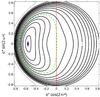 |
Fig. 6 Energy levels of the secular Hamiltonian (45) in the plane (e∗cos2ω∗ – e∗sin2ω∗) for the family of solutions of the standard system. The dashed green line shows the kinematic transition from oscillation to circulation. |
Moreover, in order to test our analytic estimations of the quasi-integrable approximation and the ratio of frequencies, we carry out three numerical simulations with different semimajor axes. We consider the standard system with the following different separations: a = 10 000 au (~0.05 pc), a = 60 000 au (i.e. ~0.3 pc), and a = 100 000 au (~0.5 pc). In Figs. 1 and 2, the three cases are indicated with red symbols as follows: a cross for a = 10 000 au, a triangle for a = 60 000 au, and a circle for a = 100 000 au. For the three examples, we plot the temporal evolution of the angle ω and the dynamical behaviour in the plane (ω,e) in Figs. 7 and 8, respectively. For a = 60 000 au the temporal evolution shows other perturbations in addition to the secular frequency and for larger semimajor axes (i.e. a> 60 000 au) our approximation is no longer valid (i.e. fo and fn are commensurable), which agrees with our analytical deduction.
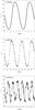 |
Fig. 7 Evolution of the angle ω for the binary system of Figs. 3 and 4, but with the following three different values of semimajor axis: a = 10 000 au (top panel), a = 60 000 au (middle panel), and a = 100 000 au (bottom panel). |
The prediction of the secular one-degree of freedom model shows a good agreement with the numerical experiments for ϵ< 0.05 and out of the region of commensurable frequencies, indicating that the model seems to be accurate enough for the approximations considered.
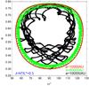 |
Fig. 8 Dynamical evolution of the binary system of Figs. 3 and 4 in the plane (ω,e), but for the following three different values of semimajor axis: a = 10 000 au (red), a = 60 000 au (green), and a = 100 000 au (black). |
3. Stationary solutions of the averaged Hamiltonian
The family of solutions in Fig. 5 shows two stable stationary solutions at (ω∗,e∗) ~ (90°, 0.54) and (270°, 0.54). Such points are equilibrium solutions (maxima or minima) of the tidal secular dynamic defined by the Hamiltonian function. From the mean-mean Hamiltonian of the one-degree of freedom model, we can find the position of the equilibrium solutions and also we are able to determine if the coupling between e∗ and I∗ (H∗ = const.) is a consequence of the Lidov-Kozai type resonance or not. In the case of a resonant behaviour there are three equilibrium points, while in a non-resonant one there is a single point (Murray & Dermott 1999).
The averaged mean-mean Hamiltonian is 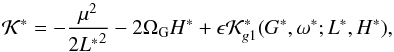 (45)where the two first terms are constant (i.e. H∗ and L∗), and the equilibrium points of the Hamiltonian are defined by the last term. Thus, our function is
 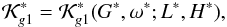 (46)with variables G∗ and ω∗.
The zero of the equations of motion are 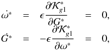 (47)where the frequency of G∗ is the derivative of the Hamiltonian with respect to the angle ω∗, and only the second term is a function of this angle (Eq. (24)). Then, the equilibrium solutions are possible for sin2ω∗ = 0 (i.e. 2ω∗ = mπ, with m = 0, 1, 2, etc.).
On the other hand, the frequency of ω∗ is the derivative of the Hamiltonian with respect to the action G∗, ![Mathematical equation: \begin{equation} \begin{array}{ccl} \dfrac{\partial \mathcal{K}^*_{g1}}{\partial G^*} &=& \dfrac{\mu^{2}}{4\,{L^*}^2} \bigg\lbrace G^* [\alpha \left(2 \cos{2 \omega^*} - 1 \right) + 1 ] \\ &&\\ &&- \dfrac{ 2 \alpha (\cos{2 \omega^*} - 1) {H^*}^2 {L^*}^2 }{{G^*}^{3}} \bigg\rbrace \, = \, 0 \rm{,} \label{eq27} \end{array} \end{equation}](/articles/aa/full_html/2017/04/aa29679-16/aa29679-16-eq191.png) (48)and solving for G∗ we obtain
(48)and solving for G∗ we obtain 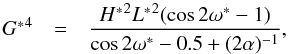 (49)with (2α)-1 ~ 0.1477. For an even multiple of π (i.e. mπ, where m = 0, 2, 4, etc.), the term cos2ω∗−1 is always 0. Hence, G∗ = 0 (e∗ = 1) and the solutions are in the limit of an hyperbolic motion. Moreover, because the coupling of e and I (i.e. H∗ = const.), there is a single value of H∗ (H∗ = 0) that satisfies such solutions. Therefore, we can discard these equilibrium points because they are not a general solution of each family and their study are out the scope of our study.
In the case of odd values of m the equilibrium points are
![Mathematical equation: \begin{eqnarray} &&{G^*_M}^2 = {H^*} {L^*} \sqrt{\dfrac{-2}{ - 1.5 + ( 2 \alpha)^{-1}}} {,} \quad \,\, 2\omega^* = m \pi \, (m=1 , 3) {,} \nonumber\\[2mm] &&{G^*_M} \sim 1.103 \sqrt{{H^*} {L^*} } {,} \qquad\qquad \qquad \omega^* = m \pi/2 \, (m=1, 3) {.} \label{eq29} \end{eqnarray}](/articles/aa/full_html/2017/04/aa29679-16/aa29679-16-eq203.png) (50)
(50)
Considering the standard system of Sect. 2.5, we found  au2/yr, or
  and ω∗ = 90 and 270° (2ω∗ = 180°), which is coincident with the maxima shown in the Fig. 5.
Therefore, we found that for each combination of H∗ and L∗ there is a single equilibrium point at 2ω∗ = 180°, whose value  in eccentricity could be interpreted as a “forced eccentricity” (ef). The forced eccentricity is a fixed value and the curves around it (e.g. ef) could be defined as a proper or free eccentricity with their own free frequency.
The existence of a single maximum indicates a similar secular (non-resonant) motion, even if the coupling between the eccentricity and the inclination seems to behave like the Lidov-Kozai resonance, but the dynamical behaviour is different because there is not a separatrix. The secular motion without resonance could be better appreciated in the plane of the regular variables x = e∗cos(2ω∗) and y = e∗sin(2ω∗), where the motion is defined as quasi-concentric circles around the forced eccentricity (). The level curves of constant mean-mean Hamiltonian of Fig. 5 (i.e. family of the standard system) are repeated in the new plane (x,y) in Fig. 6, where the absence of a separatrix is evident. In fact, we have quasi-concentric circles with the centre separated from the origin.
The difference between the dynamical structures of resonant and non-resonant motion allows us to understand why this Hamiltonian is only secular (Murray & Dermott 1999). Indeed, although the angles could oscillate in both cases, the oscillations are topologically different. In the resonant case the transition of the angle from oscillation to circulation occurs through true bifurcations of the solutions, along the separatrix that contains a saddle-like point. In other words, the two regimes of motions, oscillations, and circulation are topologically distinct. In this case, we can say that the resonant angle librates and the system is in a true resonance state. In the other case (our study case) the oscillations are merely kinematic since all levels, even those passing through the origin (green dashed curves), belong to the same structurally stable family. In other words, there is no topological difference between oscillations and circulations.
Finally, a two-body system that is disturbed by a third body is able to develop a resonance of Lidov-Kozai (Lidov 1961; Kozai 1962; Antognini & Thompson 2016). In this work we are dealing with a similar problem, where a binary system is disturbed by an external force, but we found a secular coupling of e and I. The difference seems to be in the form of the third body; in three star systems the disturbing body is a point mass, while we are working with a potential corresponding to an extended body (i.e. the Galaxy).
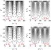 |
Fig. 9 Structure of the secular phase space of the standard system for the following four different values of the DPAM (J = H∗/L∗): 0.1 and –0.1 (top panels), and 0.3 and –0.3 (bottom panels). The left panels show the (ω∗−e∗) plane, and the right panels show the (ω∗−I∗)-plane. Although the dynamical structure is similar, the position of the equilibrium points in the e∗-axis (and I∗-axis) and the extension of the phase space decrease with the increase of J. |
4. Dynamical portait of the secular evolution
In the previous section we analysed the energy levels of a particular set of values for H∗ and L∗, which we named a “family”, and now we consider other families to provide a complete description of the dynamical portrait of the problem. Since  , a better option is to work on fixing the value of L∗, which allows us to introduce the variable
 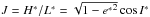 (i.e. a dimensionless projection of the angular momentum, DPAM), which varies between –1 to 1.
Then, for the masses and initial value of L of the standard system, we chose eight different values for DPAM: J = −0.7, –0.5, –0.3, –0.1, 0.1, 0.3, 0.5, and 0.7, which are represented in Figs. 9 and 10. However, the Galactic potential is symmetric in the z-axis; in fact the equilibrium points (Eq. (49)) and the equations of motion (47) have a quadratic dependence on H∗. Thus, the secular phase space of the binary system depends on the absolute value of H∗ or J. Therefore, we represent the eight DPAM in four dynamical maps, one for each positive-negative pair of J. In order to make a more complete dynamical analysis, we represent each map in two planes: the (ω∗−e∗)-plane and (ω∗−I∗)-plane.
We can see that the general structure of the phase space does not change and there are two maxima for mean-mean Hamiltonian at ω∗ = 90° and 270°. The most important differences between the eight maps are the following: first, the position of the equilibrium points of the Hamiltonian, which decreases in eccentricity (and I∗) when J increase; second, smaller values of J allow greater values of eccentricity (and I∗) and the extension of the phase space increase in the e∗ direction (I∗ direction). We are working with mean-mean variables, but we choose the initial value of L as our mean-mean value L∗, which is possible because of the small amplitude of the action variables L and H (see Sect. 2.5).
Next, we changed the value of L∗, keeping fixed J (H∗/L∗) in 0.5 (Fig. 10, top panel). However, L∗ depend on the masses and the semimajor axis, and then we choose three test cases with a = 100 and 50 000 au, and m2 = 0.8M⊙. Figure 11 shows our results (black line), where the levels of constant mean-mean Hamiltonian for a = 10 000 au (i.e. Fig. 10, top panel) were included for comparison (dashed red line). The dynamical structure is equal in the three cases, and it agrees very well with the example of reference (dashed red lines).
 |
Fig. 10 Same as in Fig. 9 except for DPAM (J = H∗/L∗): 0.5 and –0.5 (top-panels), and 0.7 and –0.7 (bottom-panels). |
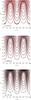 |
Fig. 11 Phase space for different values of L∗: a∗ = 100 (top panel), 50 000 au (middle panel), and m2 = 0.8 M⊙ (bottom panel). As comparison the levels of constant Hamiltonian for a = 10 000 au of the Fig. 10 (top panel) are indicated with dashed red line. |
The independence of the dynamic structure with the variable L∗ is a very important result, which indicates that the long-period dynamics of a binary system in the Galaxy depends on the z component of the angular momentum (H), but it is independent of the semimajor axis and the masses (L). Because of such independence of the masses, the dynamical behaviour for any binary system (i.e. star-star, Sun-comet, etc.) is always the same for similar values of DPAM (J).
Such results can be analytically deduced from the mean-mean Hamiltonian,  (51)The two first terms of the Hamiltonian are constants, thus solving for
  we can define a new Hamiltonian,
![Mathematical equation: \begin{equation} \mathcal{K}_J \, = \, \epsilon \dfrac{\mu^{2}}{4\,{L^*}^2} \left[ \alpha \left(\sin{{I^*}}\right)^2 \left(1+{e^*}^2 - {e^*}^2 \cos{2\omega^*}\right) - \left(1+{e^*}^2\right) \right] \rm{.} \label{eq31} \end{equation}](/articles/aa/full_html/2017/04/aa29679-16/aa29679-16-eq229.png) (52)Since ϵL∗-2μ2/ 4 is a constant, we can move it to the left side and we obtain a new Hamiltonian, which is only function of e∗ and I∗, and is written as
(52)Since ϵL∗-2μ2/ 4 is a constant, we can move it to the left side and we obtain a new Hamiltonian, which is only function of e∗ and I∗, and is written as  (53)Then, although the absolute value of the Hamiltonian
  changes for different values of a∗ or the masses, its functional form depends only on the eccentricity and inclination, which explains the agreement in Fig. 11.
However, the influence of the Galactic potential is only reported for wide binary systems (Brunini 1995; Jiang & Tremaine 2010), and it is ignored for tight binary systems (a< 1000 au). Therefore we could explore these systems looking for the dependence of the potential with the separation. We find that the difference lies in the period of the tidal secular cycle. From the Eq. (51), the Hamilton equations are ![Mathematical equation: \begin{equation} \begin{array}{ccl} \dot{\omega^*} = \epsilon \dfrac{\partial \mathcal{K}^*_{g1}}{\partial G} &=& \epsilon \dfrac{\mu^{2}}{4\,{L^*}^2} \bigg\lbrace G^* [\alpha (2 \cos{2 \omega^*} - 1 ) + 1 ] \\ &&- \dfrac{ 2 \alpha (\cos{2 \omega^*} - 1) {H^*}^2 {L^*}^2 }{{G^*}^{3}} \bigg\rbrace \rm{,} \\ \dot{G^*} = - \epsilon \dfrac{\partial \mathcal{K}^*_{g1}}{\partial \omega} &=& - \epsilon \dfrac{2 \alpha \mu^{2}}{4\,{L^*}^2\,{G^*}^2} ({L^*}^2 - {G^*}^2) ( {G^*}^2 -{H^*}^2) \sin{2 \omega^*} \rm{.} \label{eq33} \end{array} \end{equation}](/articles/aa/full_html/2017/04/aa29679-16/aa29679-16-eq233.png) (54)Once again, working algebraically we obtain
(54)Once again, working algebraically we obtain ![Mathematical equation: \begin{equation} \begin{array}{ccl} \dot{\omega^*} &=& \Omega_{\rm G} A_{\rm G} \dfrac{{L^*}^3}{\mu^{2}} \bigg\lbrace \sqrt{1-{e^*}^2} [\alpha (2 \cos{2 \omega^*} - 1 ) + 1 ] \\[3mm] &-& \dfrac{ 2 \alpha (\cos{2 \omega^*} - 1) {(\cos I^*)}^2 }{\sqrt{1-{e^*}^{2}}} \bigg\rbrace \, \rm{,}\\[3mm] \dot{G^*} &=& - 2 \Omega_{\rm G} A_{\rm G} \alpha \dfrac{{L^*}^4}{ \mu^2} {e^*}^2 (\sin I^*)^2 \sin{(2 \omega^*)} \rm{.} \label{eq34} \end{array} \end{equation}](/articles/aa/full_html/2017/04/aa29679-16/aa29679-16-eq234.png) (55)Thus, the functional form of the evolution of the variables ω∗ and G∗ is the same and similar to the mean-mean Hamiltonian, it is independent of the semimajor axis and the masses. However, the terms L∗3μ-2 and L∗4μ-2 in
(55)Thus, the functional form of the evolution of the variables ω∗ and G∗ is the same and similar to the mean-mean Hamiltonian, it is independent of the semimajor axis and the masses. However, the terms L∗3μ-2 and L∗4μ-2 in  and
and  , respectively, change the frequency of the secular cycle. It is worth to note that, the evolution of ω∗ is dimensionless, but is parametrized by L∗. So, the motion equations and
  are a better choice to understand the dynamical difference between binary systems.
For the modified motion equations ( and  ), the tidal secular period is defined by L∗3μ-2 (a∗1.5μ-0.5). These results allow us to understand the difference between tight and wide binary systems with similar masses. The dynamical behaviour is the same for any binary system, but the time required to complete the secular cycle changes as a function of the separation and the masses of the components of the pair.
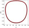 |
Fig. 12 Secular phase space of the standard system for a = 10 000 au (black line) and a = 1000 au (red line), in the plane (ω,G/L). Because we find good agreement between the two binary systems, we decided to reduce the size of the red curve to appreciate the black curve. |
The analytic result deduced from Eq. (55) is illustrated by the standard system of Sect. 2.5. For the binary star with masses m1 = 1.0 M⊙ and m2 = 0.3 M⊙, we consider two configurations: aA = 10 000 au and aB = 1000 au. From our one-degree of freedom model, in the modified motion equations ( and ) we can predict a relation between the secular periods as ![Mathematical equation: \begin{equation} \begin{array}{ccccccl} \dfrac{\dot{\omega^*_B}}{\dot{\omega^*_A}} &=& \dfrac{T_A}{T_B} &\sim& ({a^*_B}/{a^*_A})^{1.5} &\sim& 0.031 \rm{,}\\[3mm] \dfrac{\dot{G^*_B}L^*_A}{\dot{G^*_A}L^*_B} &=& \dfrac{T'_A}{T'_B} &\sim& ({a^*_B}/{a^*_A})^{1.5} &\sim& 0.031 \rm{.} \label{eq35} \end{array} \end{equation}](/articles/aa/full_html/2017/04/aa29679-16/aa29679-16-eq249.png) (56)Then, the wide binary star (10 000 au) has a secular period ~31 times smaller than the tidal period of the more compact binary star (1000 au).
(56)Then, the wide binary star (10 000 au) has a secular period ~31 times smaller than the tidal period of the more compact binary star (1000 au).
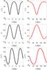 |
Fig. 13 Temporal evolution of the orbital elements I (top panels), e (middle panels) and ω (bottom panels) of the standard system: a = 10 000 au (left panels) and a = 1000 au (right panels). |
In order to test our theoretical predictions, we consider some numerical examples. From Sect. 2.5, we know that the temporal evolution of the osculating (G, ω) and mean-mean (G∗, ω∗) action-angle variable are similar. Then, in Figs. 12 and 13 we show the dynamical behaviour of first, the standard system (10 000 au) and, second, a modify standard system (1000 au). The structures of both systems have similar dynamical behaviours, which can be seen in the plane (ω,G/L) in Fig. 12. However, the temporal evolution of ω and G/L in Fig. 13 show different secular periods for each one. For clarity, it is easier to work with the eccentricity than with G/L, so in Fig. 13 we represent the evolution of e (middle panels) and to give a more complete picture we also include the evolution of I (top panels). We can see that the standard system completes the cycle in 5 Gyr (top panel), but the modify standard system (bottom panel) has a period of 160 Gyr, with a relation of 160/5 ~ 32, which confirms our prediction. The implication of this result is that a binary system with a< 1000 au have a dynamical behaviour similar to that shown by a wide binary (a> 1000 au), but the period of the first system has a Galactic tidal cycle longer than the age of the universe, which is in agreement with our theoretical predictions, and cannot be detected in real systems.
The other variables (or parameters) in L∗ are the masses of each body, m1 and m2. The dependence of the secular frequency with these parameters is weaker than the dependence with the semimajor axis. This is because the range of possible masses is smaller than the range in a (i.e. between 10 and 0 M⊙), and the dependence of the secular period with the semimajor axis has a steeper slope than with the masses. As an example, we consider the standard system of Sect. 2.5 with a central body of 1 M⊙ and semimajor axis 10 000 au, but we change the mass of the secondary: 0.8 M⊙ (A), 0.3 M⊙ (B), and 0.001 (C) M⊙. The theoretical prediction of the ratio between their tidal secular periods in  is
is 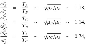 (57)respectively. The same difference is obtained for the frequency of G∗/L∗. So, the difference is small and the long tidal periods for different binary systems such as star-star, star-planet, or even Sun-comet is similar. Figure 14 shows the temporal evolution of the osculating angle ω for the three examples, where, once again, we consider the temporal evolution of the osculating elements similar to the mean-mean action-angle variable (Sect. 2.5). The numerical determined periods are A: ~6.1 Gyr, B: ~ 5.2 Gyr and C: ~4.5 Gyr, with a ratio between these periods that confirms our theoretical prediction.
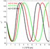 |
Fig. 14 Comparison of the temporal evolution of ω for a standard system with m2: 0.8 (A, green line), 0.3 (B, red line), and 0.001 (C, black line) M⊙. |
Then, the total mass of the binary system (i.e. m1 + m2) is not important and has a negligible influence in the dynamical evolution of the system in the Galaxy. This is an important result because it shows that the one-degree of freedom model can be applied to different binary systems (i.e. star-star, planet-star, Sun-comet, etc.) with similar results.
Finally, from our study we can deduce that the DPAM, J, defines the structure of the phase space and the scale parameter L∗ regulates the temporal evolution of the binary system in the Galaxy. So, for each value of J there is a maximum in the Hamiltonian, and from Eq. (50) we can obtain the position of such maximum in the plane (e∗, I∗). In this way, different values of J define a curve of equilibrium points in the plane (e∗, I∗), which can be defined as a “family of equilibrium solutions” (FES). Figure 15 shows the position of all the equilibrium solutions calculated for the scale parameter L∗ of the standard system of Sect. 2.5. We can see that J increases when e∗ and I∗ decrease. For simplicity we plotted only the positive values of J because owing to the potential symmetry the curve is similar for I< 0°. The structure of the FES in the plane (e∗,i∗) is equal for any value of L∗ because it has no influence in the dynamic behaviour of the binary systems.
5. Application to the problem of stellar collisions
The collision of the components of a wide binary star system due to the perturbation of the Galaxy (Kaib & Raymond 2014) is an interesting problem to which we can apply the predictions of our model. The tidal field of the Milky Way influences the pericentre distance (q) of the system, forcing close passages between the components of the pair.
For a collision a close encounter between the components of the binary system at a distance less than the combined radii of the stars is necessary. The range of radii considered in Kaib & Raymond (2014) is ∈ (0.13, 4.4) R⊙. Then, the minimum distance of pericentre is equal to the combined radius of the stars as follows: qm = R1 + R2. According to the range of radii, the distance qm has a maximum of ~8.8 R⊙ for two massive stars, and a minimum of ~0.26 R⊙ for late-type stars. Moreover, the separation between the stars in Kaib & Raymond (2014) has a range of values ∈ (1000, 30 000) au. These two distances (i.e. a and qm) define the parameter 1−e = qm/a, which regulates the probability of a collision.
We can define two limits of probability for the collision: an upper limit of maximum probability for massive stars with a = 1000 au and a lower probability limit for late-type stars separated by 30 000 au. These limits give us a critical value for the eccentricity of 1−ec1 ~ 4 × 10⁻⁵ in the first case and 1−ec2 ~ 4 × 10⁻⁸ in the second case.
According to our one-degree of freedom model, the parameter that regulates the secular phase space of any binary system in the Galaxy is J. This parameter is defined as  , which together with ec and the limit of the cosine function (i.e. | cosI | < 1) define the probability of collision of a particular binary star system.
In both cases, ec1 and ec2, the maximum value of the relation  is 1, which corresponds to I = 0°. This give us the critical values | Jc1 | ~ 0.01 and | Jc2 | ~ 3 × 10⁻⁴.
Because the whole secular phase space is in the range | J | ∈ (0,1), the limits | Jc1 | and | Jc2 | indicate the fraction of the phase space where a collision is possible. Then, we can consider | Jc1 | and | Jc2 | as the maximum and minimum probabilities of collision (i.e. PM and Pm) of each system. Because we are considered two limit cases, the probability of collision for any other binary stars systems is between | Jc1 | and | Jc2 | (i.e. between PM and Pm).
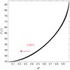 |
Fig. 15 Position of the maxima for all the possible values of J (FES) for the L∗ of the standard system in the plane (e∗,i∗). We can see that J (H∗) increases with the decrease of e∗ and I∗. |
We note that for a particular value of J, there is a secular plane of motion associated; see Figs. 9 and 10. Then, for particular values | Jc1 | and | Jc2 |, not all the orbits in the plane achieve the high eccentricities necessary to collide, and it is very difficult to estimate the percentage of close encounters in each plane. Thus, for the sake of simplicity we give an approximate 50% probability of each plane. This estimation reduces the maximum PM and minimum Pm probabilities by a factor two. Hence, we can conclude that a particular wide binary star system has a probability between 1 in 200 and 1 in 6000 of having a close encounter that ends in a collision between their components. Finally, although we have not considered stellar passages and tidal forces between the stars, our analytical results are in agreement with the empirical collision probability found by Kaib & Raymond (2014).
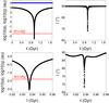 |
Fig. 16 Temporal evolution of a binary system with small pericentre distance, similar to that of Fig. 1 in Kaib & Raymond (2014). In the top left panel we plot the semimajor axis (blue line) and the pericentre distance (black line). The red line indicates the limit of stellar collision. The top right panel shows the inclination. Bottom panels show a zoom over the minimum distance of approach between the stars. |
As an application example of the prediction of our model, we carry out two numerical simulations by integrating the exact equations of motion through a Bulirsch-Stoer code with an adopted accuracy of 10-13. For example, we consider the binary system of Fig. 1 of Kaib & Raymond (2014) with two stars of 1 M⊙ each, where a = 10 000 au and q0 = 1000 au (i.e. initial pericentre distance). From the prediction of our one-degree of freedom model, this system has a collision probability of ~0.001, which indicates that J ≤ 0.001. Then, we arbitrarily choose J = 8 × 10⁻⁴, which, combined with the initial eccentricity (0.9), allow us to calculate the initial inclination, I0 ~ 89.7°. Our model also predicts that the angles M and Ω can be chosen randomly because they are fast angles related to the secular period. We chose an initial value of 0 for the angle ω because at 90° it achieves the minimum pericentre distance. However we can randomly choose any value between 0 and 80, close to the minimum q. It is worth noting the simplicity of the process to define the required initial conditions through the one-degree of freedom model.
Moreover, we consider another example with same masses and semimajor axis, but an initially circular orbit (i.e. q0 = 10 000 au). The aim of this second example is to show the importance of the Galaxy even in circular orbits, according to the prediction of our model. The Jc is equal, so we consider the same value of J used to calculate the inclination. The angle ω is zero and the other two angles are randomly defined.
Figures 16 and 17 show the temporal evolution of the semimajor axis, the pericentre distance and the inclination for both examples. The red line shows the distance of collision between the stars. Although we do not consider stellar passages and the dynamical tidal force between the stars, the isolated effect of the Galactic potential allows us to deduce important conclusions:
-
The fast angles are not important for the problem and, although weshow one example for each simulation here, we have tested othervalues with identical results.
-
The two systems spend most of the time separated by most of 100 au and at high inclination (I> 88°).
-
The time of approach between the stars is short compared with the total secular cycle and the inclination only decreases in such instances.
These conclusions seem to indicate that the most important condition for a close approach between the stars are the high inclination between the orbital plane and the mid-plane of the Galaxy.
From these conclusions, we can say that the secular model is an important tool to obtain fast results in wide binary systems. Through our model we are able to estimate the percentage of the system that ends in collision and also we easily found initial conditions that end in a collision between the stars.
6. Conclusions
In this paper, we found an analytic one-degree of freedom model for the secular evolution of a binary system in the Galactic environment of the solar neighbourhood. With this model, we develop a detailed dynamic portrait of the phase space of a binary system affected by the tidal field of the Galaxy.
The simple secular model was obtained through an averaging process (Morbidelli 2002; Ferraz-Mello 2007) applied to the three-dimensional Galactic potential of Binney & Tremaine (2008). The mean-mean Hamiltonian and corresponding equations of motion allow a fast calculation of the secular evolution of binary systems with a low computational cost, despite a fast characterization of the phase space. We note that our reduced model is useful not only for binary stars systems, but also for restricted two-body problems (i.e., star-comet, star-planet, etc.).
On the other hand, we found that the structure of the phase space of binary systems disturbed by the tidal field of the Galaxy is only dependent on the angular momentum and is independent of the masses and the separation of the pair. Moreover, the quasi-conservation of the z component of the angular momentum gives a dynamical structure similar to the Lidov-Kozai resonance, but without the presence of a separatrix (i.e. there is not a resonant motion). This result has two important consequences for studies of binary systems: first, the Galaxy can excite the astrocentric orbit of the companion from a circular initial orbit to a high eccentric orbit (Sect. 5), and, second, in the limit of application of this simple model we do not find a source of chaos in the secular behaviour (i.e. there is not separatrix), therefore the disruption of the pair seems to be unlikely.
However, the secular periods change as a function of the semimajor axis (a). Then, binary systems with lower separation between their components have higher secular periods than more separated pairs. This result is very important because it represents an analytical dynamical interpretation for the empirical limit of ~1000 au that separates “wide” and “tight” binary systems. For object couples with separations lower than 1000 au, the secular tidal period is greater than the age of the universe.
We also apply our model for the study of a specific problem: stellar collision in wide binary stars systems. We have found that the secular model allows us to estimate quickly the region of the phase space where a close approach is possible. Moreover, these results may have an important application for studies of planetary systems in wide binary stars.
Finally, we have determined a limit of the application of our model, which depends on the masses and separation between the components of the binary. For very separated binary systems with small masses, the model loses precision. So, the simplifications are no longer valid and we must consider the three-dimensional complete model.
Acknowledgments
The authors are grateful to an anonymous referee for numerous suggestions and corrections that have helped to improve this paper.
References
- Antognini, J. M. O. 2015, MNRAS, 452, 3610 [NASA ADS] [CrossRef] [Google Scholar]
- Antognini, J. M. O., & Thompson, T. A. 2016, MNRAS, 456, 4219 [NASA ADS] [CrossRef] [Google Scholar]
- Bahcall, J. N., Hut, P., & Tremaine, S. 1985, AJ, 290, 15 [Google Scholar]
- Binney, J., & Tremaine, S. 2008, Galactic Dynamics 2nd edn. (Princeton University Press) [Google Scholar]
- Brouwer, D., & Clemence, G. M. 1961, Methods of celestial mechanics (New York: Academic Press) [Google Scholar]
- Brunini, A. 1995, A&A, 293, 935 [NASA ADS] [Google Scholar]
- Eggers, S., & Woolfson, M. 1996, MNRAS, 282, 13 [NASA ADS] [CrossRef] [Google Scholar]
- Ferraz-Mello, S. 2007, Canonical Perturbation Theories: Degenerate Systems and Resonance (Springer Press) [Google Scholar]
- Fouchard, M., Froeschlé, C., Valsecchi, G., & Rickman, H. 2006, Mech. Dyn. Astron., 95, 299 [Google Scholar]
- Heggie, D. C. 1975, MNRAS, 173, 729 [NASA ADS] [CrossRef] [Google Scholar]
- Heggie, D. C. 2001, in The Restless Universe, eds. B. A. Steves, & A. J. Maciejewski, 109 [Google Scholar]
- Heisler, J., & Tremaine, S. 1986, Icarus, 65, 13 [NASA ADS] [CrossRef] [Google Scholar]
- Jiang, Y. F., & Tremaine, S. 2010, MNRAS, 401, 977 [NASA ADS] [CrossRef] [Google Scholar]
- Kaib, N. A., & Raymond, S. N. 2014, ApJ, 782, 60 [NASA ADS] [CrossRef] [Google Scholar]
- Kaib, N. A., Roskar, R., & Quinn, T. 2011, Icarus, 215, 491 [NASA ADS] [CrossRef] [Google Scholar]
- Kaib, N. A., Raymond, S. N., & Duncan, M. 2013, Nature, 493, 381 [NASA ADS] [CrossRef] [Google Scholar]
- Kozai, Y. 1962, AJ, 67, 591 [Google Scholar]
- Levison, H. F., & Dones, L. 2001, AJ, 121, 2253 [NASA ADS] [CrossRef] [Google Scholar]
- Lidov, M. L. 1961, Iskusst. sputniky Zemly 8, Acad. of Sci., USSR [Google Scholar]
- Michtchenko, T. A., Lazzaro, D., Ferraz-Mello, S., & Roig, F. 2002, Icarus, 158, 343 [NASA ADS] [CrossRef] [Google Scholar]
- Morbidelli, A. 2002, Modern Celestial Mechanics: aspects of solar system dynamics (CRC Press) [Google Scholar]
- Murray, C. D., & Dermott, S. F. 1999, Solar system dynamics (Cambridge University Press) [Google Scholar]
- Naoz, S. 2016, ARA&A, 54, 441 [Google Scholar]
- Naoz, S., Farr, W. M., Lithwick, Y., Rasio, F. A., & Teyssandier, J. 2013, MNRAS, 431, 2155 [NASA ADS] [CrossRef] [Google Scholar]
- Roell, T., Neuhäuser, R., Seifahrt, A., & Mugrauer, M. 2012, A&A, 542, A92 [NASA ADS] [CrossRef] [EDP Sciences] [Google Scholar]
All Figures
|
Fig. 1 Level curves of constant ϵ in the plane (a, m1 + m2). The dotted red line indicates the limit for the integrable approximation. The approximation fails for the binary systems below the dashed blue line. The red symbols (cross, triangle, and circle) represent the position of three binary systems (see Sect. 2.5). |
| In the text | |
|
Fig. 2 Level curves of the ratio between the frequencies: fo/fs (dashed black line), fn/fs (dotted blue line) and fo/fn (red line). For the comparison with the secular frequency we plot the ratio 1 and 10. For the comparison between the fast frequencies (fo/fn) we plot the levels 1, 2, 5 and 10. The red symbols (cross, triangle and circle) represent the position of three binary systems (see Sect. 2.5). |
| In the text | |
|
Fig. 3 Time evolution of the action variables of Delaunay L (top panel), H (middle panel) and G (bottom panel) for our standard system. The small variations of L and H and the circulation of M and Ω (Fig. 4) confirm the proposed approximation. |
| In the text | |
|
Fig. 4 Time evolution of the angular variables of Delaunay M (top panel), Ω (middle panel) and ω (bottom panel) for our standard system. The small variations of L and H (Fig. 3) and the circulation of M and Ω confirm the approximation proposed. |
| In the text | |
|
Fig. 5 Comparison between the predictions of our model (dashed black line) and numerical simulations (red and blue lines) in the plane (ω∗,e∗), for the family of solutions of the standard system. |
| In the text | |
|
Fig. 6 Energy levels of the secular Hamiltonian (45) in the plane (e∗cos2ω∗ – e∗sin2ω∗) for the family of solutions of the standard system. The dashed green line shows the kinematic transition from oscillation to circulation. |
| In the text | |
|
Fig. 7 Evolution of the angle ω for the binary system of Figs. 3 and 4, but with the following three different values of semimajor axis: a = 10 000 au (top panel), a = 60 000 au (middle panel), and a = 100 000 au (bottom panel). |
| In the text | |
|
Fig. 8 Dynamical evolution of the binary system of Figs. 3 and 4 in the plane (ω,e), but for the following three different values of semimajor axis: a = 10 000 au (red), a = 60 000 au (green), and a = 100 000 au (black). |
| In the text | |
|
Fig. 9 Structure of the secular phase space of the standard system for the following four different values of the DPAM (J = H∗/L∗): 0.1 and –0.1 (top panels), and 0.3 and –0.3 (bottom panels). The left panels show the (ω∗−e∗) plane, and the right panels show the (ω∗−I∗)-plane. Although the dynamical structure is similar, the position of the equilibrium points in the e∗-axis (and I∗-axis) and the extension of the phase space decrease with the increase of J. |
| In the text | |
|
Fig. 10 Same as in Fig. 9 except for DPAM (J = H∗/L∗): 0.5 and –0.5 (top-panels), and 0.7 and –0.7 (bottom-panels). |
| In the text | |
|
Fig. 11 Phase space for different values of L∗: a∗ = 100 (top panel), 50 000 au (middle panel), and m2 = 0.8 M⊙ (bottom panel). As comparison the levels of constant Hamiltonian for a = 10 000 au of the Fig. 10 (top panel) are indicated with dashed red line. |
| In the text | |
|
Fig. 12 Secular phase space of the standard system for a = 10 000 au (black line) and a = 1000 au (red line), in the plane (ω,G/L). Because we find good agreement between the two binary systems, we decided to reduce the size of the red curve to appreciate the black curve. |
| In the text | |
|
Fig. 13 Temporal evolution of the orbital elements I (top panels), e (middle panels) and ω (bottom panels) of the standard system: a = 10 000 au (left panels) and a = 1000 au (right panels). |
| In the text | |
|
Fig. 14 Comparison of the temporal evolution of ω for a standard system with m2: 0.8 (A, green line), 0.3 (B, red line), and 0.001 (C, black line) M⊙. |
| In the text | |
|
Fig. 15 Position of the maxima for all the possible values of J (FES) for the L∗ of the standard system in the plane (e∗,i∗). We can see that J (H∗) increases with the decrease of e∗ and I∗. |
| In the text | |
|
Fig. 16 Temporal evolution of a binary system with small pericentre distance, similar to that of Fig. 1 in Kaib & Raymond (2014). In the top left panel we plot the semimajor axis (blue line) and the pericentre distance (black line). The red line indicates the limit of stellar collision. The top right panel shows the inclination. Bottom panels show a zoom over the minimum distance of approach between the stars. |
| In the text | |
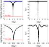 |
Fig. 17 Same as Fig. 16, but for a system with an initially circular orbit. |
| In the text | |
Current usage metrics show cumulative count of Article Views (full-text article views including HTML views, PDF and ePub downloads, according to the available data) and Abstracts Views on Vision4Press platform.
Data correspond to usage on the plateform after 2015. The current usage metrics is available 48-96 hours after online publication and is updated daily on week days.
Initial download of the metrics may take a while.