| Issue |
A&A
Volume 600, April 2017
|
|
|---|---|---|
| Article Number | A5 | |
| Number of page(s) | 11 | |
| Section | The Sun | |
| DOI | https://doi.org/10.1051/0004-6361/201629589 | |
| Published online | 17 March 2017 | |
A relaxation model of coronal heating in multiple interacting flux ropes
1 School of Mechanical, Aerospace, and Civil Engineering, University of Manchester, Manchester M13 9PL, UK
e-mail: This email address is being protected from spambots. You need JavaScript enabled to view it.
2 Jodrell Bank Centre for Astrophysics, School of Physics and Astronomy, University of Manchester, Manchester M13 9PL, UK
3 School of Mathematics and Statistics, University of St. Andrews, St. Andrews, Fife, KY16 9SS, UK
Received: 28 August 2016
Accepted: 22 December 2016
Abstract
Context. Heating the solar corona requires dissipation of stored magnetic energy, which may occur in twisted magnetic fields. Recently published numerical simulations show that the ideal kink instability in a twisted magnetic thread may trigger energy release in stable twisted neighbours, and demonstrate an avalanche of heating events.
Aims. We aim to construct a Taylor relaxation model for the energy release from two flux ropes and compare this with the outcomes of the simulations. We then aim to extend the model to large numbers of flux ropes, allowing the possibility of modelling a heating avalanche, and calculation of the energy release for ensembles of twisted threads with varying twist profiles.
Methods. The final state is calculated by assuming a helicity-conserving relaxation to a minimum energy state. Multiple scenarios are examined, which include kink-unstable flux ropes relaxing on their own, as well as stable and unstable flux ropes merging into a single rope as a result of magnetic reconnection. We consider alternative constraints that determine the spatial extent of the final relaxed state.
Results. Good agreement is found between the relaxation model and the magnetohydrodynamic simulations, both for interactions of two twisted threads and for a multi-thread avalanche. The model can predict the energy release for flux ropes of varying degrees of twist, which relax individually or which merge through reconnection into a single flux rope. It is found that the energy output of merging flux ropes is dominated by the energy of the most strongly twisted rope.
Conclusions. The relaxation approach provides a very good estimate of the energy release in an ensemble of twisted threads of which one is kink-unstable.
Key words: magnetohydrodynamics (MHD) / magnetic reconnection / Sun: corona / Sun: flares / Sun: magnetic fields
© ESO, 2017
 Open Access article, published by EDP Sciences, under the terms of the Creative Commons Attribution License (http://creativecommons.org/licenses/by/4.0),
which permits unrestricted use, distribution, and reproduction in any medium, provided the original work is properly cited.
Open Access article, published by EDP Sciences, under the terms of the Creative Commons Attribution License (http://creativecommons.org/licenses/by/4.0),
which permits unrestricted use, distribution, and reproduction in any medium, provided the original work is properly cited.
1. Introduction
The solar corona is heated to temperatures of several million degrees Kelvin through dissipation of magnetic energy. A promising scenario, especially for closed magnetic structures, or loops, is that stored magnetic energy is efficiently dissipated through the process of magnetic reconnection. Reviews of our current understanding of coronal heating are provided by Parnell & De Moortel (2012) and Klimchuk (2015), while the role of reconnection in coronal heating is reviewed by Longcope & Tarr (2015). The coronal magnetic field contains free energy if it is non-potential, and an elemental non-potential field is a twisted magnetic flux rope. Energy storage and release in twisted fields is representative of processes operating in more complex non-potential fields, and twisted flux ropes are likely to be common in the solar corona, arising both from emergence of twisted fields from the solar interior and through the action of footpoint motions with vorticity.
The ideal kink instability can trigger the onset of fast magnetic reconnection in a twisted flux rope, releasing stored magnetic energy and heating the plasma (Browning & Van der Linden 2003; Browning et al. 2008; Hood et al. 2009; Bareford et al. 2013). There are many observations of kink instability in the solar corona, manifesting as small confined flares; see, for example, Liu et al. (2007), Liu & Liu (2009), Srivastava & Dwivedi (2010), Wang et al. (2015). Nevertheless, it is unlikely that, at any point in time, the majority of coronal flux will be sufficiently twisted to be kink-unstable. Thus, effective energy release requires dissipation of energy from some magnetic flux ropes that are stable.
There is increasing observational evidence of multi-thread structures within observed coronal loops. From a theoretical point of view, the “flux tectonics” picture (Priest et al. 2002) suggests that a single large loop may have its footpoints rooted in several discrete photospheric flux sources. Twisting within the individual flux sources will lead to a closely-packed array of twisted flux ropes, separated by current sheets. A natural consequence will be reconnection at the current sheets, causing the flux ropes to merge, with associated heating as magnetic energy is dissipated. An alternative scenario is that photospheric motions with vorticity will twist up separate elements of a magnetic flux tube (e.g. De Moortel & Galsgaard 2006). Thus, the coronal magnetic field is likely to be non-potential, consisting of a large number of current-carrying threads (twisted magnetic flux ropes in the simplest situation), often interspersed by current sheets.
The merger of two or more twisted flux ropes into a single structure has long been considered as a possible mechanism for the release of stored magnetic energy; causing both large-scale flares, and, on smaller scales, coronal heating (Gold & Hoyle 1960; Melrose 1997; Kondrashov et al. 1999). There are, broadly, two possible approaches: in the first, the twisted flux ropes carry a net current and thus attract each other, while in the second, the flux ropes are in full equilibrium, thus requiring some instability or external driving to trigger merging. The former is relevant to many laboratory flux rope merging experiments, since the currents are inductively driven by external coils; merger in this situation has been modelled numerically by Stanier et al. (2013), with application to the MAST spherical tokamak. We focus here on the latter case, in which the twisted flux ropes are initially in equilibrium. The question then arises as to how the reconnection required for flux rope merger can be triggered.
Recently, it has been shown using 3D magnetohydrodynamic (MHD) simulations that one kink-unstable flux rope can trigger energy release in a stable neighbour (Tam et al. 2015). If the two ropes are initially sufficiently close, the unstable rope interacts with the stable one, releasing free magnetic energy from both flux ropes, with the two ropes merging through magnetic reconnection into a single twisted flux rope. This has important implications for coronal heating, since stored energy can be released even if a flux rope is stable. Subsequently, Hood et al. (2016) considered a set of 23 twisted loops, one unstable, with the remaining 22 loops stable, showing that the onset of instability in the one unstable loop triggered a series of mergers with the stable neighbours, with bursty energy release as the loops merge in turn. Such a scenario has been widely proposed in the context of Cellular Automaton (CA) models (e.g. Lu & Hamilton 1991; Charbonneau et al. 2001), but this was the first demonstration using 3D MHD simulations of an “avalanche”.
Such numerical simulations are very computationally demanding, and it is not viable to explore a wide parameter space. For this reason, it would be very useful to have a simpler, semi-analytical model. In order to understand solar coronal heating, the small-scale dynamics of the magnetic reconnection process are not important, rather we are only required to know the magnetic energy that can be dissipated. To this end, the approach of relaxation theory, following Taylor (1974, 1986), provides a powerful tool.
The idea that a stressed magnetic field undergoes a helicity-conserving relaxation to a minimum energy state was first applied to the coronal heating problem by Heyvaerts & Priest (1984). It is proposed that the coronal magnetic field is stressed by photospheric footpoints, and subsequently relaxes to a minimum energy state, which is a constant-α or linear force-free field, with the released magnetic energy heating the coronal plasma. This approach has been widely applied in the subsequent literature. One outstanding issue in the Heyvaerts and Priest theory was the question of how much the free energy builds up before the onset of relaxation. Browning & Van der Linden (2003) proposed that, in a twisted magnetic flux rope, relaxation could be triggered by the onset of the ideal kink instability. Subsequent 3D MHD numerical studies (Browning et al. 2008; Hood et al. 2009; Bareford et al. 2013) essentially confirmed this prediction, showing that a fragmented current sheet forms during the nonlinear phase of the kink instability. This leads to multiple reconnections of the magnetic field lines, which reduce the twist and allow the field to relax to a lower energy state, which is well approximated by Taylor theory. The relaxation approach was then used to model distributions of heating events caused by varying the current profile (Bareford et al. 2010, 2011), predicting a power-law-like distribution of nanoflares and providing effective coronal heating rates.
A relaxation model of reconnecting twisted flux ropes was recently developed by Browning et al. (2014), with application to merging-compression formation in the MAST spherical tokamak, and then applied to interacting solar coronal flux ropes (Browning et al. 2016). However, the initial state in this model represents adjacent flux ropes separated by current sheets, which does not address the onset conditions for flux rope merger and cannot readily be applied to the situation modelled numerically by Tam et al. (2015) and Hood et al. (2016).
Our aim here is to develop a relaxation model in which the initial state consists of a number of twisted magnetic threads in force-free equilibrium. The final relaxed state as the threads interact, and potentially merge, is determined using Taylor theory. The approach is developed and tested for a pair of flux tubes, and benchmarked against the 3D mumerical simulations of Tam et al. (2015). The methodology is set out in Sect. 2, with results presented in Sect. 3. Then, in Sect. 4, we extend the model to a system with a large number of flux ropes, making a comparison with the numerical results of Hood et al. (2016). Conclusions are presented in Sect. 5.
2. Theoretical approach and methodology
2.1. Initial field configuration
Our aim is to consider the interactions of a number of discrete twisted magnetic threads that are initially in force-free equilibrium. Therefore, following Tam et al. (2015) and Hood et al. (2016) we model each individual thread as a cylindrical force-free flux rope (radius Ri and length L) with zero net-current (see also Melrose 1991; Hood et al. 2009; Bareford et al. 2011).Thus, the azimuthal field Bθ is zero at the edge of the flux rope. In between the threads, there is a uniform axial field Bz = Be. Initially, all fields are continuous, so that Bz(Ri) = Be. We non-dimensionalise the equations by setting:  (1)We set the initial radius Ri = 1. Since our model is one-dimensional, the length is only a linear scaling factor, but for comparison with previous work, we specifically set L = 20. To non-dimensionalise the analysis, the magnetic permeability is also set to unity (μ0 = 1). Comparisons requiring numerical values are obtained by considering typical parameters for a coronal loop, for example, B0 = 0.01 T, ρ = 1.67 × 10⁻¹² kg m-3, and L0 = 1 Mm; a single unit of energy represented in this work corresponds to 7.96 × 10¹⁹ J ( ≈1020 J).
In order to develop and benchmark the model, we first consider two initial flux ropes, but later (Sect. 4) we extend this to multiple flux ropes. A suitable model for the initial field, allowing direct comparison of our relaxation model with numerical simulations, is given by Hood et al. (2009), Tam et al. (2015): ![Mathematical equation: \begin{eqnarray} \label{eq:BTheta} B_{\theta}&=&\begin{cases} \begin{array}{c} B_{0}\lambda r(1-r^{2})^{3},\\ 0, \end{array} & \begin{array}{c} r\leq1\\ r>1, \end{array}\end{cases}\\ \label{eq:ExactBz} B_{z}&=&\begin{cases} \begin{array}{c} \! \! \! B_{0}\sqrt{1\!-\!\frac{\lambda^{2}}{7}\!+\!\frac{\lambda^{2}}{7}(1\!-\!r^{2})^{7}\!-\!\lambda^{2}r^{2}(1\!-\!r^{2})^{6}},\\[2mm] \! \! \! B_{0}\sqrt{1-\frac{\lambda^{2}}{7}}. \end{array} & \begin{array}{c} \! \! \! \! \! r\leq1\\[2mm] \! \! \! \! \! r>1, \end{array}\end{cases}\\ \label{eq:ExactBr} B_{r}&=&0. \end{eqnarray}](/articles/aa/full_html/2017/04/aa29589-16/aa29589-16-eq17.png) The initial magnetic field is chosen to be force-free (i.e. j × B = 0). Since the flux rope arises from localised twisting at the photospheric footpoints, the azimuthal field (Bθ) must vanish at the edge of the rope (hence the field is continuous with the surrounding purely axial field). Thus, by Ampere’s law, the net axial current along the loop must vanish. Indeed, the axial current associated with the fields in Eq. (2)changes sign between the centre of loop (r = 0) and the edge (r = 1), allowing the net current to be zero (see Hood et al. 2009). Hence, the configuration arises as a result of localised twisting within the two regions of the photosphere. The parameter λ quantifies the twist in the flux rope. One observes this relationship by considering the angle of rotation of a field line from one end of the loop to the other,
The initial magnetic field is chosen to be force-free (i.e. j × B = 0). Since the flux rope arises from localised twisting at the photospheric footpoints, the azimuthal field (Bθ) must vanish at the edge of the rope (hence the field is continuous with the surrounding purely axial field). Thus, by Ampere’s law, the net axial current along the loop must vanish. Indeed, the axial current associated with the fields in Eq. (2)changes sign between the centre of loop (r = 0) and the edge (r = 1), allowing the net current to be zero (see Hood et al. 2009). Hence, the configuration arises as a result of localised twisting within the two regions of the photosphere. The parameter λ quantifies the twist in the flux rope. One observes this relationship by considering the angle of rotation of a field line from one end of the loop to the other, 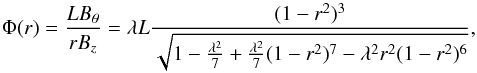 (5)hence the twist on axis r = 0 is simply
  (6)In order to ensure that each flux rope has an identical field at r = 1, allowing continuity with the surrounding uniform field, it is required that
  (7)is the same for each flux rope, where Be is the external field (a constant axial field). Be is set to 0.7329, which corresponds to B0 = 1 and λ = 1.8.
As the twist is increased, the ropes will become kink-unstable. Previous calculations, taking line-tying at the ends of the flux ropes (Hood & Priest 1979; Bareford et al. 2010) into account, show that the ropes are linearly-unstable to the ideal kink mode at λcrit = 1.586. Note that this value will change if the aspect-ratio L/Ri is changed. There is a strict upper limit on the allowable value of λ, since Bz must be real (λmax = 2.438).
The magnetic helicity (K) is defined as:  (8)where A is the magnetic vector potential, such that ∇ × A = B. Since the loop is not fully bounded by a magnetic surface, the expression for helicity must be adjusted to ensure gauge-invariance (Berger 1984; Finn & Antonsen Jr. 1985). The most convenient implementation of the gauge-correction for a geometry such as ours, in which the field at the two ends of the loop z = 0 and L is identical, is to consider the loop to be a periodic system, that is, an infinite-aspect ratio torus. The necessary “gauge-correction” term arising due to an unspecified flux through the torus can be made to vanish by specifying Az(R) = 0, where R is the loop radius (Bevir et al. 1985; Browning et al. 2014).
The aim here is to have an analytical model. However, given the form of the profile for Bz, the vector potential cannot be found analytically. Therefore, a polynomial approximation for Bz up to the 7th order is used. This is shown to provide a high degree of accuracy in Sect. 2.5. Such an approximation was used instead of numerical integration since calculation of helicity requires repeated integration, and it is convenient to have explicitly analytic expressions for the various quantities. This approximation is only used to provide expressions for the helicity and the axial flux; other quantities such as energy can be calculated directly from Eq. (3). Therefore, Bz is given by: 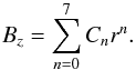 (9)The coefficients are determined by using a least squares polynomial fit after evaluating the field for a specific λ.
After some algebra, detailed in Appendix A, the expressions for the magnetic energy (E), axial flux (Ψ), and helicity are obtained. ![Mathematical equation: \begin{eqnarray} E&=&B_{0}^{2}\pi L \left(\frac{1}{2}-\frac{\lambda^2}{16}\right),\\[-0.5mm] \Psi&=&2\pi\int^{R_i}_0 B_z r.{\rm d}r = 2\pi\sum_{n=0}^{7}\frac{C_{n}}{n+2}, \end{eqnarray}](/articles/aa/full_html/2017/04/aa29589-16/aa29589-16-eq46.png) and
and 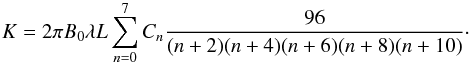 (12)It should be noted in all the above expressions that, for fixed external field Be, the field on the flux rope axis, B0 is given as a function of λ according to Eq. (6). Thus, magnetic energy is indeed an increasing function of twist (λ).
For a system of multiple threads, the energy, axial flux, and helicity are determined as the summation of the individual quantities for each flux rope. Note that the external (current-free) field makes no contribution to helicity, but does affect the total energy and axial flux – although the latter quantities will only alter if the volume of this region changes (since the field Be is uniform and unchanging); this is discussed further in Sect. 2.2.
2.2. Relaxed state
The Taylor relaxation model (Taylor 1974, 1986) determines the lowest energy state obtainable with the total helicity conserved. This predicts a magnetic field, which is a linear force-free field (∇ × B = αB) with the value of α determined by the constraints that the helicity and axial flux (Ψ) are the same as in the initial state. This is usually accomplished by conserving the dimensionless ratio K/ Ψ2. In a cylindrical configuration, the relaxed state is given by  (13)where B1 is a constant (the magnitude of the relaxed field on axis) and J0 and J1 are the zeroth and first order Bessel functions of the first kind.
In the following, we assume that the relaxed state is a cylindrical flux tube with radius Rf. The external (potential) field remains unaltered during the relaxation process. Unlike the laboratory situation, relaxation in the solar corona is a free boundary problem (Dixon et al. 1989). The simulations strongly suggest that the relaxed field is a flux tube of approximately circular cross-section, and it is likely that a circular boundary should give lowest energy (by analogy, for example, with the shape of bubbles).
The external field outside the flux ropes is unchanged during the relaxation process. It should be noted that, in general, the full field configuration in the relaxed state thus contains a current sheet at the flux rope boundary (the magnetic field is discontinuous). This is observed to some extent in simulations, although the sheet becomes a layer of finite width (see also Bareford et al. 2013). A current sheet is also predicted in models of localised relaxation applied to the edge region of tokamaks (Gimblett et al. 2006).
For the relaxed state (Eq. (13)), the normalised helicity, with the gauge-invariance condition Az(Rf = 0), can thus be shown to be ![Mathematical equation: \begin{equation} \frac{K}{{\Psi}^{2}}=\frac{L}{2\pi R_{f}}{\frac{\alpha R_{f}[J_{0}^{2}(\alpha R_{f})+J_{1}^{2}(\alpha R_{f})]-2J_{0}(\alpha R_{f})J_{1}(\alpha R_{f})}{J_{1}^{2}(\alpha R_{f})}}, \end{equation}](/articles/aa/full_html/2017/04/aa29589-16/aa29589-16-eq57.png) (14)(in agreement with Taylor 1974, 1986).
(14)(in agreement with Taylor 1974, 1986).
2.3. Relaxation calculation
We begin by developing the relaxation model to represent as closely as possible the 3D MHD simulations undertaken by Tam et al. (2015), thus testing and benchmarking the approach. As in Tam et al. (2015), four cases for the initial field, each with two ropes, were considered. The cases vary in terms of the twist λ, and whether or not they merge in a magnetic reconnection event (which in the simulations is controlled by the distance between the threads). In the simulations, merging occurs when the two flux ropes initially just touch at a single line (i.e. the centre of the second flux rope is exactly 2Ri away from the centre of the first). If the flux ropes are sufficiently separated, they do not interact and it is likely that there is a maximum separation below which interaction occurs. The Taylor relaxation model does not explicitly model the location of the initial flux ropes, but we can specify whether the final state should be a single flux rope, or whether the flux ropes should relax individually, in order to compare with the relevant simulations.
In order to provide direct comparison with the numerical results, a “simulation box” can be defined. The simulation box is defined as a rectangular cross-section region outside the flux ropes with a uniform axial magnetic field 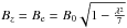 , of dimensions 8 by 4 by 20. When a simulation box is used, the total energy of the system includes a contribution from the external field. A simulation box setup is illustrated for cases 2 and 4 in Fig. 1. The energy of the external region remains unchanged if the volume of the flux tubes remains constant, but may change otherwise.
 |
Fig. 1 Azimuthal field lines of flux ropes as initially setup a) and then relaxing to form a single flux rope b) in an 8 × 4 × 20 simulation box. The final state depicted is specific to cases 2 and 4. |
As discussed above, the relaxed state is assumed to be cylindrical but it is not immediately clear what the radius of the final flux rope should be. Simulations of the relaxation of a single unstable twisted flux tube show that the relaxed state has limited extent a little larger than the initial flux tube, which is a form of “partial relaxation” (Bareford et al. 2013). Thus, initially, we considered the outcomes of the relaxation model treating the final radius (Rf) as an unspecified variable, with the energy change recorded accordingly. Various approaches were then used to determine the final radius. The first is simply a conservation of volume (thus the total cross-sectional area of the initial and final flux ropes is the same). The second is equating the magnetic pressure to the background magnetic pressure (which is unchanged during the relaxation process, as the external field is unchanging), which is illustrated in Eq. (2). The third constraint takes account of the fact that the dissipated magnetic energy is converted into thermal energy and, hence, the gas pressure inside the flux rope increases, and should be added to the magnetic pressure. This is illustrated in Eq. (17), where an ideal gas has been assumed and γ is the adiabatic index. Constraints 2 and 3 maintain force balance across the interface between the twisted flux rope and the external field. Constraint 1 has no particular physical justification but is simple to apply and appears to match the simulations quite well, and will be shown to produce rather similar results in terms of energy released.
To summarise, the radius is constrained by:
-
Constraint 1: conservation of volumebetween the initial and final flux ropes,
 (15)
(15) -
Constraint 2: equating magnetic pressure at the edge of the final flux rope to the background magnetic pressure,
 (16)
(16) -
Constraint 3: equating the sum of magnetic pressure at the edge of the final flux rope and built up gas pressure to the background magnetic pressure,
 (17)
(17)
The methodology is then as follows. An initial field is selected, as described in Sect. 2.4. The value of α in the final state is calculated by equating the helicity of the final flux rope (normalised with respect to axial flux – which is also conserved) to the total helicity of the initial flux ropes (Eq. (12)), for a given radius of the final flux rope, Rf. For the constraints 2 and 3, Rf is iterated to achieve the required pressure balance. The energy release, which is presumed to be converted into plasma thermal energy, is then simply the difference between the energy of the initial state and the final state.
2.4. Cases studied
In order to benchmark the relaxation model, we first develop it for the same cases studied numerically by Tam et al. (2015). The various cases for the initial field considered are given in Table 1.
Initial field conditions for the relaxation of two flux ropes.
Thus cases 1 and 2 have two unstable flux ropes, while in cases 3 and 4, one flux rope is unstable and the other is stable – hence the latter will not release any energy unless somehow disrupted.
In cases 2 and 4, the flux ropes merge into a single flux rope. In cases 1 and 3, the unstable flux rope (λ = 1.8) relaxes individually to constant state.
Later, in Sect. 4, we also consider a much larger array of flux ropes, representing the avalanche situation simulated in Hood et al. (2016).
2.5. Validation of field approximation
We first check the accuracy of the polynomial approximation to the axial field profile (Eq. (9); see Fig. 2). Here, excellent agreement is shown between the approximation to the field (Eq. (3)) and the exact force-free field.
 |
Fig. 2 a) Approximating polynomial and exact function for axial field Bz(r), demonstrating the quality of fit, for λ = 0.8 (approximate, green, and exact, blue), λ = 1.4 (approximate, red, and exact, cyan), λ = 1.8 (approximate, violet, and exact, khaki). Note that only three curves are visible since the exact and approximate curves are almost identical. b) The difference between the exact and the approximation function for λ = 1.8. |
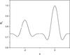 |
Fig. 3 Initial axial field Bz for two flux ropes, using the approximate polynomial, for case 4; the flux ropes centred at (0,0) and (− 2,0). |
Within Fig. 2, one observes that the fit is very good since only three curves can be visually observed despite six being plotted, which allows confidence in using the approximation. Further confidence is provided by matching the Bz profiles (Fig. 3) to the ones in Tam et al. (2015).
The initial total magnetic energy for cases 1 and 2 was found to be 175.52 and for cases 3 and 4 to be 174.37 (in dimensionless units). These are in good agreement with the associated values reported in Tam et al. (2015).
3. Results
3.1. Effect of the radius of final flux rope
Initially, the radius Rf of the final flux rope was varied to observe the dependence of the energy output on this quantity, bearing in mind that the relaxation is a “free surface problem” in the corona. Figure 4 shows the energy release from two flux ropes merging into one (as in cases 2 and 4) as a function of the final radius, Rf. Similarly, Fig. 5 shows the energy released due to a single flux rope relaxing (as in the case of the unstable flux ropes in cases 1 and 3). The energy is calculated both with a “simulation box” (in which the magnetic energy of the external region varies) and without (in which only the energies of the flux ropes are included).
Results of the Taylor model compared to the MHD model.
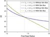 |
Fig. 4 Energy change for two flux ropes merging and relaxing against final rope radius, both with (green, λ1 = 1.4λ2 = 1.8; cyan, λ1 = λ2 = 1.8) and without (blue, λ1 = 1.4λ2 = 1.8; red, λ1 = λ2 = 1.8) a simulation box. Positive values represent an increase in energy from the initial to final state. The vertical line represents conservation of volume. |
If two flux ropes relax into a single rope, and volume is conserved, the radius of the final flux rope will be  , as indicated by the vertical line in Fig. 4. Note that if the volume is conserved (which is similar to the situation in a laboratory plasma confined within a rigid container), the energy change is negative – as expected for a relaxation to a minimum energy state. In this case, we expect that the released magnetic energy is converted into thermal energy. Initially, as demonstrated in simulations (Browning et al. 2008; Hood et al. 2009; Tam et al. 2015) some magnetic energy is converted into kinetic energy associated with reconnection outflows, but this is viscously dissipated as a relaxed state is approached. If the flux tube volume decreases significantly, the magnetic energy rises, due to the increase in energy caused by compression dominating the decrease due to relaxation; we do not expect this situation to arise in practice (as some external work would need to be done to compress the flux ropes). Conversely, there is an increasing conversion of magnetic energy into heat as the flux tube volume increases.
Furthermore, note that when volume is conserved, the cases with and without “simulation box” are identical – because the axial field external to the flux ropes is unchanged in both magnitude and volume through the relaxation, and hence makes no contribution to the energy change. The released energy depends quite strongly on the choice of final radius, and we now consider the possible ways in which this can be determined.
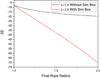 |
Fig. 5 Energy output for a single flux rope relaxing (λ = 1.8) against final rope radius (Rf) with (green) and without (blue) a simulation box. |
3.2. Calculation of energy release and comparison with simulations
We now apply the three constraints that might determine the radius of the relaxed flux rope, as set out in Sect. 2.3 (Eqs. (15)to (17)).
For constraints 2 and 3, the radius is determined by iterating Rf until the appropriate pressure balance is attained. The energy release is calculated for initial fields for each of the four cases, which can then be compared with the outcomes of the 3D numerical simulations Tam et al. (2015). The latter are calculated as the difference in magnetic energy between the initial value and that at the end of the simulation; we note that this has some margin of uncertainty, since the energy is still changing to some extent. From Table 2, it can be seen that there is generally good agreement between the numerical MHD result and the relaxation model. Also, the calculated energy release does not depend strongly on the choice of constraint. Some discrepancies between the numerical energy release and the relaxation predictions arise; both because the numerical simulations do not necessarily achieve full relaxation by the end of the simulation and because the expansion in loop radius observed numerically for a single relaxing loop is not fully accounted for by any of our constraints. The final radius for two merging loops is much better predicted by our model (all constraints giving little change in volume) than for a single loop.
Constraint 3 is arguably the most physically correct, as it accounts for the loop expansion due to plasma heating. However it is quite complex numerically, as it requires multiple stages of numerical iteration. The energy release predicted by the relaxation model in this case is somewhat larger than the numerical value: this may be because the fully relaxed state is not attained by the end of the numerical simulations. Constraint 1 (constant volume), on the other hand, has no clear physical justification, but is simple to apply, and the calculated energy release agrees relatively closely with the other constraints. Therefore, this could be useful in future modelling. Here, we choose to use Constraint 2 in the following sections, as this gives the best agreement with the numerical results and is relatively simple to apply. We may also compare the predicted final radius from the three constraints with the outcome of the MHD simulations; however, it is difficult to measure this accurately from the simulations, and this cannot be used to discriminate between the three proposed constraints. It does appear that when an individual flux rope relaxes (as in cases 1 and 3), there is a clear expansion of the rope, which has been suggested to be approximately 1.2 times the initial radius (Bareford et al. 2013). The analysis of Bareford et al. (2013) suggests that this is due to the unstable twisted flux rope reconnecting with the surrounding axial field and thus “eating into” the untwisted field region. This effect is not accounted for in our model, although it could be. The extent of this expansion is determined essentially by the nonlinear amplitude of the kink instability, but at present, we have no way to predict this a priori, and this is a subject for future investigation.
In general, there is very good agreement between the energy changes predicted by the relaxation model and the outcomes of the simulation. Furthermore, there is a very clear consistency in the trends of variation between the different cases.
3.3. The dependence of energy release on initial fieldline twist
The major advantage of the relaxation approach is that the energy can be calculated easily for a wide parameter space, and thus (in contrast with numerical simulations, which are very demanding of computer resources), we can explore how coronal heating varies with the paramaters of the twisted flux ropes. Thus, having benchmarked the approach against the simulations, we now investigate how the energy release varies with the flux rope twist, quantitified by the parameter λ. We thus calculate the energy change for the full range of possible initial twists for a pair of flux ropes. For each pair of λ values, the initial energy and helicity are calculated as described in Sect. 2.1 above (with the set of coefficients Cn determined for each λ). The external field Be is held fixed, so that the peak axial field B0 is determined by Eq. (6). The flux ropes are assumed to merge, relaxing to a single constant-α flux rope. The resulting energy change is illustrated in the form of a contour map in Fig. 6. Note that, in order for relaxation to happen at all, at least one flux rope must be unstable, so the region in which both values of λ are less than approximately 1.6 should be excluded.
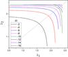 |
Fig. 6 Contours of energy change for two flux ropes merging and relaxing with various λ. The dotted line represents λ2 = λ1. |
As one can observe, the contours depict an increasing output of energy for higher overall twist. Furthermore, the energy output seems to be dominated by the contribution of a highly unstable flux rope, as the contours are closely parallel to the x and y axes, respectively, for larger twist. We also note that the energy output rises strongly as λ increases towards its upper limit (i.e. λmax = 2.438, beyond which Bz becomes imaginary), tending to infinity at this limit. However, whilst the general increase of energy release with field line twist is entirely expected, this singular behaviour is an artefact of the chosen mathematical model. The dependence of energy change on twist is further shown in Fig. 7, which considers two identical initial flux ropes λ = λ1 = λ2 (corresponding to the dotted line in Fig. 6). Figure 8 shows the variation of the force-free parameter (α) with varying twist; the other flux rope is fixed at λ = 1.8. One can observe that the parameter increases as the twist increases.
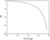 |
Fig. 7 Energy output as a function of twist for two initially identical flux ropes λ = λ1 = λ2. |
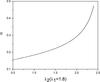 |
Fig. 8 Variation of α vs. λ2, where λ1 is fixed at 1.8. |
4. Large multi-threaded flux ropes
One strength of the Taylor model is its ease of applicability to larger regions, and more complex initial fields, without an increase in computational requirements. Hood et al. (2016) used 3D MHD simulations to demonstrate an avalanche of heating in an array of 23 twisted flux ropes, consisting of one unstable rope surrounded by stable ropes. However, such simulations are highly demanding of computational resources. We, therefore, consider this situation using the relaxation approach. The initial conditions were set to have one central flux rope unstable at λ = 1.8 surrounded by stable flux ropes, λ = 1.4, as depicted in Fig. 9. In the simulation described by Hood et al. (2016), an avalanche was observed as the unstable flux rope “absorbs” the other flux ropes in a cascading sequence, releasing energy from the stable twisted flux ropes in succession.
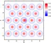 |
Fig. 9 Simulation setup for 23 flux ropes merging. The figure shows current density in the midplane z = L/ 2, taken from the early stage of the MHD simulations. The central rope is the unstable flux rope (λ = 1.8) while the rest are stable (λ = 1.4). Note that the central unstable flux rope shows signs of the initial kink instability, with a current sheet forming at the right-hand side of the loop. Originally published in Hood et al. (2016). |
The approach in applying the Taylor model is similar to the preceding work; at each stage, the individual energies and helicities are calculated, then superimposed to find the total value. However, we now extend the approach described for two flux ropes in Sect. 3 to superimpose the flux ropes one at a time, providing a direct comparison to the avalanche model. Thus, first a stable flux rope and an unstable one are relaxed into a single flux rope (as in case 4 above). Then, this is combined with a further stable flux rope, and relaxed into a new combined (larger) flux rope – and so on. At each stage, helicity is conserved, and the energy change is evaluated. The results are presented in Table 3, and illustrated in Fig. 10. For these purposes, it is assumed that each relaxation takes the same time, and this timestep has been chosen to match the overall time for the simulations.
Results of the Taylor model compared to the MHD model for the 23 flux rope simulation.
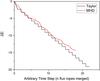 |
Fig. 10 Energy release from merging of individual flux ropes showing the MHD simulation (green) and relaxation model (blue). The arbitrary time step depicts the number of flux ropes that have been absorbed into the reconnection process. The MHD time has been normalised to scale to the Taylor model. This is needed since the Taylor model does not provide a time factor. |
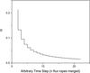 |
Fig. 11 Variation of force-free parameter, α, for the avalanche model. |
In this case, the Taylor and MHD models are seen to be in very good agreement. It is further observed that the energy drop between each step is slowly approaching a constant energy release. A possible explanation is as follows. The Taylor model assumes a fully relaxed state. As each additional stable flux rope (which are identical, with λ = 1.4) is absorbed, almost all the free energy of this rope is released. Once the energy output is dominated by the λ = 1.4 flux ropes rather than the single unstable (λ = 1.8) one, then the energy output is simply directly proportional to the number of flux ropes merged. It is noted that in the MHD simulation, only 18 flux ropes merged. It is unclear whether or not there would be further merging if the simulation were run for longer. However, this could not be checked without risking inconsistency due to numerical errors. One possible explanation for the termination of the avalanche is provided, however, by observing the force-free parameter (α) for the avalanche model (Fig. 11). As one can observe, the parameter appears to have an exponential-type decay. This suggests that as it approaches a minimum value, the current sheet surrounding the relaxed field (the Taylor model is not zero at the edge therefore resulting in an azimuthal current sheet) will become very weak after a large number of threads have merged, and no longer be sufficient to cause a disruption in the neighbouring flux ropes.
5. Discussion and conclusions
We have presented a model for the energy released as one, two or many twisted flux ropes relax, and in (some cases) merge into a single flux rope, based on a helicity-conserving relaxation as hypothesised by Taylor (1974). A direct comparison shows that the Taylor model and 3D MHD simulations (Tam et al. 2015) are in good agreement. This has been demonstrated for various cases of pairs of twisted flux ropes. Furthermore, the relaxation model has been successfully compared with a 23-flux-rope simulation, showing excellent agreement with the outcomes of numerical simulations by Hood et al. (2016).
The model is based on the concept that relaxation and energy release may be triggered by kink instability in a single unstable flux rope. This may trigger the release of stored magnetic energy from neighbouring magnetic threads which are stable. This scenario has important consequences for understanding how the solar corona is heated. The avalanche of heating will occur if the threads are sufficiently close together, but the exact conditions under which the avalanche proceeds (or stops) should be a topic of further investigations. What is important is that sometimes a large number of threads may release their energy, whilst in others, only one or two threads release energy. Thus, a distribution of heating events, or “nanoflares”, of different sizes, is expected. Furthermore, within an individual avalanche, the heating is bursty and time dependent. The relaxation model can easily predict the energy release, for given initial and onset conditions (number of threads merging, number of unstable threads and so on).
One challenge in applying relaxation models to the solar corona – as opposed to laboratory plasmas – is that solar coronal fields have no conducting walls and, thus, calculation of the relaxed state is a “free boundary problem” (Browning 1988; Dixon et al. 1989). We assume here that the final relaxed state has circular cross-section – which indeed appears to be the case in the numerical simulations. However, some means to predict the radius of this flux rope must be provided. We propose that this is determined by pressure balance at the boundary between the flux rope and ambient field, and calculate this both allowing for the increase in thermal pressure due to magnetic energy dissipation, and also without this effect (considering magnetic pressure only). One observation that warrants further investigation is the fact that the volume of the flux ropes is very well conserved when magnetic pressure is assumed to balance at the boundary. If it could be demonstrated that this applies more generally in all flux tube mergers, this would be an interesting result and provide simpler conditions for future analysis. In the case of a single unstable flux rope relaxing, the final relaxed state has been shown to have somewhat larger radius – for a range of initial twist profiles, this has been shown to be typically approximately a factor of 1.2 times the initial radius (Bareford et al. 2013). This is attributed to the unstable flux rope reconnecting with the surrounding axial field, an effect which we do not consider here. Future work is required to further investigate the factors that determine the radius of the final flux rope. Nevertheless, our predictions based on magnetic pressure balance are in good agreement with simulations.
Relaxation in unbounded systems can also be interpreted as a localised relaxation (Bareford et al. 2013), in which the relaxation extends over a limited region. Indeed, it is important to recall that Taylor theory predicts only the lowest energy state that could be attained, and that full relaxation may be not be achieved. For example, when the initial field has a braided structure, numerical simulations demonstrate that the final relaxed state consists of two parallel weakly twisted flux ropes, each of which approximately corresponds to a Taylor state, but which do not merge into the lower energy overall constant-α field (Pontin et al. 2011). Furthermore, two flux ropes with opposite twist will release more energy if they relax than if the twists were in the same sense (Browning et al. 2016); but it is less likely that the relaxation will happen in this case, since the azimuthal fields at the interface between the ropes do not reverse. However, if one of the flux ropes is kink-unstable, the helical distortion may be sufficient to allow reconnection, although the reconnection may be slower in this case. Further investigations with 3D MHD simulations are required to determine the conditions under which twisted flux ropes merge into a Taylor state.
It is worth noting that a consequence of allowing relaxation over a localised region is that a current sheet (usually) must form between the relaxed field and the ambient axial field (Gimblett et al. 2006; Bareford et al. 2013). Indeed, there is evidence of such a reversed current layer in the 3D numerical simulations (Bareford et al. 2013; Tam et al. 2015; Hood et al. 2016), although naturally the current layers in this case have finite width. In the case of multiple flux ropes, it appears that this current layer plays a role in the merger of adjacent threads as the avalanche proceeds (Hood et al. 2016).
There are naturally some discrepancies between the outcomes of numerical simulations and the theoretical predictions. On the one hand, the simulated fields may not attain a fully relaxed state, as this depends on there being sufficient small-scale turbulence and reconnection throughout the volume to dissipate the free energy and re-distribute the currents. Thus, the energy release predicted by relaxation theory is an upper bound on the actual energy release. The final state in the numerical simulations is still full of small scale current sheets, and the spatial distribution of α does not appear to be particularly constant. Nevertheless, the magnetic fields (which average over the small scale current structure) are relatively well represented by constant-α fields, and the final energy is even better approximated by the relaxed-state value, since small departures from a mimimum-energy state give quadratic deviations in energy. The predicted energy release also depends on the size of the relaxed flux tube. Our model seems to under-estimate this somewhat (particularly in the case of a single relaxing flux rope, as discussed above), and this effect causes the predicted energies to be lower than the actual values.
The successful development of this model could potentially pave the way for determining outputs of larger and more complex systems, allowing more realistic modelling (potentially) of Active Regions of the solar corona. This is because the Taylor model is not restricted by the number of ropes simulated, particularly due to the fact that the system is setup as a simple superposition in the case of multiple flux ropes. This allows for very rapid calculation times, regardless of system size. Thus, it would be easy to simulate large numbers of flux ropes, with variations in size, and twisted to different degrees (including the possibility of twists of opposing sign, which are readily accounted for in the relaxation model). In future, we propose to use further numerical simulations to devise simple “rules” as to when flux ropes merge or not, and then to use these to simulate complex systems of flux ropes.
Acknowledgments
The authors wish to recognise funding from EPSRC through the Fusion Centre for Doctoral Training (FusionCDT grant code: EP/K504178/1) through which this project is possible. Support from STFC for PKB and AWH is also acknowledged (grant numbers ST/L000768/1 and ST/N000609/1).
References
- Bareford, M. R., Browning, P. K., & Van der Linden, R. A. 2010, A&A, 521, A70 [NASA ADS] [CrossRef] [EDP Sciences] [Google Scholar]
- Bareford, M. R., Browning, P. K., & Van der Linden, R. A. M. 2011, Sol. Phys., 273, 93 [NASA ADS] [CrossRef] [Google Scholar]
- Bareford, M. R., Hood, A. W., & Browning, P. K. 2013, A&A, 550, A14 [NASA ADS] [CrossRef] [EDP Sciences] [Google Scholar]
- Berger, M. A. 1984, Geophys. Astrophys. Fluid Dyn., 30, 79 [NASA ADS] [CrossRef] [Google Scholar]
- Bevir, M. K., Gimblett, C. G., & Miller, G. 1985, Phys. Fluids, 28, 1826 [NASA ADS] [CrossRef] [Google Scholar]
- Browning, P. 1988, J. Plasma Phys., 40, 263 [NASA ADS] [CrossRef] [Google Scholar]
- Browning, P. K., & Van der Linden, R. A. M. 2003, A&A, 400, 355 [NASA ADS] [CrossRef] [EDP Sciences] [Google Scholar]
- Browning, P. K., Gerrard, C., Hood, A. W., Kevis, R., & Van der Linden, R. A. M. 2008, A&A, 485, 837 [NASA ADS] [CrossRef] [EDP Sciences] [Google Scholar]
- Browning, P. K., Stanier, A., Ashworth, G., McClements, K. G., & Lukin, V. S. 2014, Plasma Physics and Controlled Fusion, 56, 64009 [CrossRef] [Google Scholar]
- Browning, P. K., Cardnell, S., Evans, M., et al. 2016, Plasma Physics and Controlled Fusion, 58, 014041 [NASA ADS] [CrossRef] [Google Scholar]
- Charbonneau, P., McIntosh, S. W., Liu, H. L., & Bogdan, T.J. 2001, Sol. Phys., 203, 321 [NASA ADS] [CrossRef] [Google Scholar]
- De Moortel, I., & Galsgaard, K. 2006, A&A, 451, 1101 [NASA ADS] [CrossRef] [EDP Sciences] [Google Scholar]
- Dixon, A., Berger, M., Priest, E., & Browning, P. 1989, A&A, 225, 156 [NASA ADS] [Google Scholar]
- Finn, J., & Antonsen, Jr., T. 1985, Comments Plasma Phys. Control. Fusion, 9, 111 [Google Scholar]
- Gimblett, C. G., Hastie, R. J., & Helander, P. 2006, Plasma Physics Controlled Fusion, 48, 1531 [NASA ADS] [CrossRef] [Google Scholar]
- Gold, T., & Hoyle, F. 1960, MNRAS, 120, 89 [NASA ADS] [Google Scholar]
- Heyvaerts, J., & Priest, E. 1984, A&A, 137, 63 [NASA ADS] [Google Scholar]
- Hood, A. W., & Priest, E. R. 1979, Sol. Phys., 64, 303 [NASA ADS] [CrossRef] [Google Scholar]
- Hood, A. W., Browning, P. K., & Linden, R. A. M. V. D. 2009, A&A, 506, 913 [NASA ADS] [CrossRef] [EDP Sciences] [Google Scholar]
- Hood, A. W., Cargill, P., Browning, P., & Tam, K. 2016, ApJ, 817, 5 [NASA ADS] [CrossRef] [Google Scholar]
- Klimchuk, J. A. 2015, Philosophical Transactions of the Royal Society A: Mathematical, Physical and Engineering Sciences, 373, 20140256 [Google Scholar]
- Kondrashov, D., Feynman, J., Liewer, P. C., & Ruzmaikin, A. 1999, ApJ, 519, 884 [NASA ADS] [CrossRef] [Google Scholar]
- Liu, J.-Y., & Liu, B.-F. F. 2009, A&A, 9, 966 [Google Scholar]
- Liu, Y., Kurokawa, H., Liu, C., et al. 2007, Sol. Phys., 240, 253 [NASA ADS] [CrossRef] [Google Scholar]
- Longcope, D. W., & Tarr, L. A. 2015, Philosophical Transactions of the Royal Society A: Mathematical, Physical and Engineering Sciences, 373, 7 [Google Scholar]
- Lu, E. T., & Hamilton, R. J. 1991, ApJ, 380, L89 [NASA ADS] [CrossRef] [Google Scholar]
- Melrose, D. B. 1991, ApJ, 381, 306 [NASA ADS] [CrossRef] [Google Scholar]
- Melrose, D. B. 1997, ApJ, 486, 521 [NASA ADS] [CrossRef] [Google Scholar]
- Parnell, C. E., & De Moortel, I. 2012, Philosophical Transactions of the Royal Society A: Mathematical, Physical and Engineering Sciences, 370, 3217 [Google Scholar]
- Pontin, D., Wilmot-Smith, A., Hornig, G., & Galsgaard, K. 2011, A&A, 525, A57 [NASA ADS] [CrossRef] [EDP Sciences] [Google Scholar]
- Priest, E. R., Heyvaerts, J. F., & Title, A. M. 2002, ApJ, 576, 533 [NASA ADS] [CrossRef] [Google Scholar]
- Srivastava, A. K., & Dwivedi, B. N. 2010, MNRAS, 405, 2317 [NASA ADS] [Google Scholar]
- Stanier, A., Browning, P., Gordovskyy, M., et al. 2013, Phys. Plasmas, 20, 122302 [NASA ADS] [CrossRef] [Google Scholar]
- Tam, K. V., Hood, A. W., Browning, P. K., & Cargill, P. J. 2015, A&A, 580, A122 [NASA ADS] [CrossRef] [EDP Sciences] [Google Scholar]
- Taylor, J. B. 1974, Phys. Rev. Lett., 33, 1139 [NASA ADS] [CrossRef] [Google Scholar]
- Taylor, J. B. 1986, Rev. Mod. Phys., 58, 741 [NASA ADS] [CrossRef] [Google Scholar]
- Wang, H., Cao, W., Liu, C., et al. 2015, Nat. Commun., 6, 7008 [Google Scholar]
Appendix A: Derivation of expressions for energy, toroidal flux and helicity
Here we detail the calculations of the relevant global quantities for the initial force-free field in an individual flux rope; all quantities are calculated in non-dimensional form and consider flux ropes of radius 1, which is an assumption of the initial magnetic field.
Energy
The magnetic energy is given by:  (18)Using
  (19)and performing the integration, the magnetic energy is given by:
  (20)
(20)
Axial flux
The axial flux must be calculated using the approximate Bz, and is given by 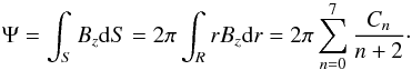 (21)
(21)
Helicity
Calculating first the vector potential A, where ∇ × A = B: 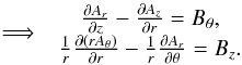 (22)
(22)
For cylindrical fields as used here, A = (0,Aθ(r),Az(r)), hence 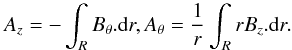 (23)Requiring that Az(r = 1) = 0, gives
 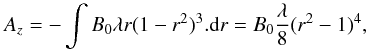 (24)and (using the approximate form of Bz)
  (25)Defining
  (26)and using
  , gives
 ![Mathematical equation: \begin{eqnarray} K&=&2\pi L B_{0}\int_{0}^{1}\left[\lambda r^{2}(1-r^{2})^{3}\sum_{n=0}^{7}\frac{C_{n}}{(n+2)}r^{n+1}\right.\nonumber \\ &&\left.\quad +\frac{\lambda}{8} (1-r^{2})^{4}\sum_{n=0}^{7}C_{n}r^{n}\right]{\rm d}r. \end{eqnarray}](/articles/aa/full_html/2017/04/aa29589-16/aa29589-16-eq107.png) (27)Multiplying out the brackets and integrating gives
(27)Multiplying out the brackets and integrating gives ![Mathematical equation: \begin{eqnarray} K&=&2\pi B_{0}\lambda L\sum_{n=0}^{7}C_{n}\Bigg[\frac{1}{8(n+2)}-\frac{1}{2(n+4)}+\frac{1}{(n+2)(n+4)}\nonumber \\ &&\quad+\frac{3}{4(n+6)}-\frac{3}{(n+2)(n+6)}-\frac{1}{2(n+8)}\nonumber \\ &&\quad +\frac{3}{(n+2)(n+8)}+\frac{1}{8(n+10)}-\frac{1}{(n+2)(n+10)}\Bigg]\nonumber \\ &=&2\pi B_{0}\lambda L\sum_{n=0}^{7}C_{n}\frac{96}{(n+2)(n+4)(n+6)(n+8)(n+10)}\cdot \end{eqnarray}](/articles/aa/full_html/2017/04/aa29589-16/aa29589-16-eq108.png) (28)
(28)
All Tables
Results of the Taylor model compared to the MHD model for the 23 flux rope simulation.
All Figures
|
Fig. 1 Azimuthal field lines of flux ropes as initially setup a) and then relaxing to form a single flux rope b) in an 8 × 4 × 20 simulation box. The final state depicted is specific to cases 2 and 4. |
| In the text | |
|
Fig. 2 a) Approximating polynomial and exact function for axial field Bz(r), demonstrating the quality of fit, for λ = 0.8 (approximate, green, and exact, blue), λ = 1.4 (approximate, red, and exact, cyan), λ = 1.8 (approximate, violet, and exact, khaki). Note that only three curves are visible since the exact and approximate curves are almost identical. b) The difference between the exact and the approximation function for λ = 1.8. |
| In the text | |
|
Fig. 3 Initial axial field Bz for two flux ropes, using the approximate polynomial, for case 4; the flux ropes centred at (0,0) and (− 2,0). |
| In the text | |
|
Fig. 4 Energy change for two flux ropes merging and relaxing against final rope radius, both with (green, λ1 = 1.4λ2 = 1.8; cyan, λ1 = λ2 = 1.8) and without (blue, λ1 = 1.4λ2 = 1.8; red, λ1 = λ2 = 1.8) a simulation box. Positive values represent an increase in energy from the initial to final state. The vertical line represents conservation of volume. |
| In the text | |
|
Fig. 5 Energy output for a single flux rope relaxing (λ = 1.8) against final rope radius (Rf) with (green) and without (blue) a simulation box. |
| In the text | |
|
Fig. 6 Contours of energy change for two flux ropes merging and relaxing with various λ. The dotted line represents λ2 = λ1. |
| In the text | |
|
Fig. 7 Energy output as a function of twist for two initially identical flux ropes λ = λ1 = λ2. |
| In the text | |
|
Fig. 8 Variation of α vs. λ2, where λ1 is fixed at 1.8. |
| In the text | |
|
Fig. 9 Simulation setup for 23 flux ropes merging. The figure shows current density in the midplane z = L/ 2, taken from the early stage of the MHD simulations. The central rope is the unstable flux rope (λ = 1.8) while the rest are stable (λ = 1.4). Note that the central unstable flux rope shows signs of the initial kink instability, with a current sheet forming at the right-hand side of the loop. Originally published in Hood et al. (2016). |
| In the text | |
|
Fig. 10 Energy release from merging of individual flux ropes showing the MHD simulation (green) and relaxation model (blue). The arbitrary time step depicts the number of flux ropes that have been absorbed into the reconnection process. The MHD time has been normalised to scale to the Taylor model. This is needed since the Taylor model does not provide a time factor. |
| In the text | |
|
Fig. 11 Variation of force-free parameter, α, for the avalanche model. |
| In the text | |
Current usage metrics show cumulative count of Article Views (full-text article views including HTML views, PDF and ePub downloads, according to the available data) and Abstracts Views on Vision4Press platform.
Data correspond to usage on the plateform after 2015. The current usage metrics is available 48-96 hours after online publication and is updated daily on week days.
Initial download of the metrics may take a while.