© ESO, 2017

1. Introduction

The exact origin of the driving mechanism of accretion disks is still not fully understood. To accrete matter onto the central object, the matter needs to lose its angular momentum, and because molecular viscosity is by many orders of magnitudes too small to facilitate the required angular transport, it has been suggested that disks are driven by turbulence. The discovery of a linear magneto-rotational instability (MRI) for rotating flows with a negative angular velocity gradient has led to the suggestion that accretion disks are driven by magnetohydrodynamical (MHD) turbulence (Balbus & Hawley 1998). However, the MRI only works efficiently for well-ionized media, for example, in disks around compact objects, but for lower ionization levels the non-ideal MHD effects become stronger and the operability of the MRI questionable. In particular for the cool and low-ionized regions, so-called dead zones with very low turbulent activity have been predicted (Gammie 1996).

Hence, other alternatives are sought for. In the past years the purely hydrodynamical vertical shear instability (VSI) has attracted some attention because the only requirement is a vertical shear in the angular velocity profile, which is in fact a natural consequence of a radial temperature gradient in the disk, for example, induced by irradiation from the central object. Through numerical simulations and linear analysis it has been shown that the VSI operates efficiently for vertically isothermal disks (Nelson et al. 2013) as well as for fully radiative disks that include stellar irradiation (Stoll & Kley 2014). This makes the VSI a promising candidate to bring at least some life back into the dead zones. For many astrophysical applications it is useful to parameterize the turbulence and describe the angular momentum transport by an effective viscous prescription, for example, the well-known ansatz by Shakura & Sunyaev (1973) where the uncertainties of the turbulence are summarized in one constant parameter α (Balbus & Papaloizou 1999). Such an approach using one parameter is applicable for an isotropic turbulence, and useful when the interest is in the overall radial evolution of the disk. To analyze the internal flow field of the disk, which is important for the motion of embedded small particles, it is necessary to take possible non-isotropy effects into account.

Here, we demonstrate that the flow reversal found in recent VSI-turbulent disks (Stoll & Kley 2016) can in fact be traced back to the intrinsic anisotropy of the VSI-turbulence. Using multidimensional hydrodynamical simulations, we calculate the effective radial and vertical transport coefficients and use them in viscous disk simulations.

2. Model setup

We use the pluto code (Mignone et al. 2007) for our simulations, where we model a section of a locally isothermal accretion disk. For the direct turbulent simulations we use a full 3D setup and spherical coordinates (R, θ, φ), while for comparison laminar viscous simulations (α-disk), we use a 2D axisymmetric setup and cylindrical coordinates (r,z). The model parameters are given in Table 1.

Even though some of the simulations are performed in spherical coordinates, the results are analyzed in cylindrical coordinates. The initial disk is axisymmetric and extends from 0.4 r₀ to 2.5 r₀, where r₀ = 5.2 au. The initial density profile is given by vertical hydrostatic equilibrium $\mathit{\rho }\mathrm{\left(}\mathit{r,z}\mathrm{\right)}\mathrm{=}{\mathit{\rho }}_{\mathrm{0}}\hspace{0.17em}{\left(\frac{\mathit{r}}{{\mathit{r}}_{\mathrm{0}}}\right)}^{\mathit{p}}\hspace{0.17em}\exp \left[\frac{\mathit{GM}}{{\mathit{c}}_{\mathrm{s}}^{\mathrm{2}}}\left(\frac{\mathrm{1}}{\mathit{R}}\mathrm{-}\frac{\mathrm{1}}{\mathit{r}}\right)\right]\mathit{,}$(1)where ρ₀ is the gas mid-plane density at r = r₀, and p = −1.5. In our locally isothermal approximation the temperature of the disk is a function of the cylindrical radius only, $\mathit{T}\mathrm{\left(}\mathit{r}\mathrm{\right)}\mathrm{=}{\mathit{T}}_{\mathrm{0}}\hspace{0.17em}{\left(\frac{\mathit{r}}{{\mathit{r}}_{\mathrm{0}}}\right)}^{\mathit{q}}\mathit{,}$(2)where we choose q = −1, which causes the disk aspect ratio to be constant and T₀ such that H/r = h = 0.05. The pressure is given by $\mathit{P}\mathrm{=}{\mathit{c}}_{\mathrm{s}}^{\mathrm{2}}\mathit{\rho }$, where c_s is the isothermal sound speed with c_s ∝ r^{− 1/2}. The gas moves initially with the angular velocity given by the Keplerian value, corrected by the pressure support (Nelson et al. 2013) $\mathrm{\Omega }\mathrm{\left(}\mathit{r,z}\mathrm{\right)}\mathrm{=}{\mathrm{\Omega }}_{\mathit{K}}{\left[\mathrm{(}\mathit{p}\mathrm{+}\mathit{q}\mathrm{)}{\left(\frac{\mathit{H}}{\mathit{r}}\right)}^{\mathrm{2}}\mathrm{+}\mathrm{(}\mathrm{1}\mathrm{+}\mathit{q}\mathrm{)}\mathrm{-}\frac{\mathit{qr}}{\sqrt{{\mathit{r}}^{\mathrm{2}}\mathrm{+}{\mathit{z}}^{\mathrm{2}}}}\right]}^{\frac{\mathrm{1}}{\mathrm{2}}}\mathit{,}$(3)with ${\mathrm{\Omega }}_{\mathit{K}}^{\mathrm{2}}\mathrm{\left(}\mathit{r}\mathrm{\right)}\mathrm{=}\mathit{G}{\mathit{M}}_{\mathrm{\ast }}\mathit{/}{\mathit{r}}^{\mathrm{3}}$, and the meridional flow (u_r,u_z) is set to zero. At the inner and outer boundary we use reflecting boundaries. To increase numerical stability for the turbulent runs, we damp the variables ρ,u_r,u_z to the initial values on a timescale of half a local orbit following the recipe by de Val-Borro et al. (2006), with a damping applied at the inner boundary from 0.4−0.5 r₀ and at the outer boundary from 2.3−2.5 r₀. At the vertical boundaries we use reflective boundaries when the flow is directed inward and zero gradient otherwise. The VSI model is inviscid, and for the α-disk model the kinematic viscosity is given by ν = 2/3αc_sH, with a constant α = 5 × 10^-4, which matches the outcome of VSI model.

3. Disk structure

We compare the structure of the VSI unstable disk to viscous disks described by an α-parameter, and study the main differences. The VSI disk is evolved to a quasi-equilibrium state before the analysis is performed. We focus in particular on the flow field and stress tensor, and refer to Nelson et al. (2013) and Stoll & Kley (2014, 2016) for an analysis of the turbulent flow structure.

While the density distributions of the viscous and turbulent disks in equilibrium are very similar due to the necessary pressure equilibrium, there is an important difference in the meridional flow within the disk in particular for the radial velocity. We show the azimuthally averaged radial velocity u_r at r = r₀ as a function of the vertical distance for the turbulent and the standard viscous disk in Fig. 1. For the turbulent disk we averaged the velocity in time over 50 orbits and in space around r₀ in the region (0.8−1.25)r₀. For better visibility we rescaled the viscous case by a factor of 200. Obviously, the two radial velocity profiles have an opposite behavior. The standard viscous disk using a single (isotropic) value of α shows the typical outflow in the midplane that has been predicted analytically by Urpin (1984) and was later shown in fully time-dependent numerical simulations (Kley & Lin 1992). This behavior of u_r(z) can be derived from the equilibrium angular momentum equation that contains the vertical disk structure (Urpin 1984). In spite of the outwardly directed flow in the midplane, the total vertically integrated mass flow is nevertheless directed inward in case of accreting disks (Kley & Lin 1992).

In contrast, the mean flow field for the turbulent flow (labeled 3D VSI and shown also with a dotted line for a model with double resolution in all directions) is fully reversed; it is not only negative in the midplane and positive in the corona, but also much stronger, as indicated by the different scaling of the curves in Fig. 1. This special feature of the meridional flow field in the VSI case has been found for isothermal as well as radiative disks in Stoll & Kley (2016), but was not analyzed with respect to anisotropic turbulence. From the direct comparison to the viscous case, it is clear that with a standard shear viscosity prescription using a constant α-value or a constant kinematic viscosity, no agreement can be obtained because this will always lead to an inverted parabolic type of profile (Jacquet 2013). This raises the general question whether the VSI turbulence in disks can be described by a standard Navier-Stokes approach to model the angular momentum diffusion. In Sect. 4 we show that we obtain a good match of a fully turbulent and viscous flow for a non-anisotropic turbulent viscosity where the radial and vertical parts enter with a different strength (see curve 2D anisotropic stress), which might be expected for the clearly non-isotropic character of the flow structure in VSI turbulence (Stoll & Kley 2014).

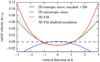Fig. 1 Radial velocity averaged over 50 orbits. We compare the disk with alpha-viscosity (α = 5 × 10-4, blue curve) to a disk with active VSI (red curve), a disk with active VSI and doubled resolution (red dotted curve) and a viscous disk with anisotropic stress similar to the VSI disk (green curve, details see Sect. 4). For the turbulent disk the velocity has been azimuthally averaged. The profile shown is in units of sound speed cs0 and at r = r0. The viscous case has been rescaled to better visualize the difference.

To analyze the effect of the turbulence with respect to angular momentum transport in the disk, it is necessary to calculate the turbulent stresses of the VSI disk. For the overall mass flow in accretion disks, which is driven by outward angular momentum transport, the rφ-component of the Reynolds stress tensor, R, is the most important component because it is generated by the strong shear in the azimuthal velocity. In the case of VSI turbulent disks, it is clear that the vertical dependence of the turbulent stresses (zφ-component) may be of importance as well. Hence, from our simulations we calculate the following turbulent Reynolds stresses 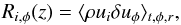${\mathit{R}}_{\mathit{i,\phi }}\mathrm{\left(}\mathit{z}\mathrm{\right)}\mathrm{=}\mathrm{⟨}\mathit{\rho }{\mathit{u}}_{\mathit{i}}\mathit{\delta }{\mathit{u}}_{\mathit{\phi }}{\mathrm{⟩}}_{\mathit{t,\phi ,r}}\mathit{,}$(4)where u_i with i in (r,z) denote the radial and vertical flow velocity (u_r,u_z) and δu_φ is the deviation of the azimuthal velocity, u_φ = rΩ, from unperturbed equilibrium, as given by Eq. (3). For the later analysis it is beneficial that the stresses are calculated in cylindrical coordinates (r,z), see Sect. 4. Since we are interested in particular in the vertical dependence of the stresses, R_i,φ is calculated by averaging over the full azimuth (2π), over a small radial range around a reference radius, and over time. Here, we time-average from orbit 80 to orbit 200 using a series of over 60 snap shots and space-average in radius from 0.75−1.35 r₀.

The results of this averaging procedure are shown in Fig. 2. The solid curves refer to the specific stresses R_i,φ(z) /ρ(r₀,z) (i = r,z) in units of ${\mathit{c}}_{\mathrm{s}\mathrm{0}}^{\mathrm{2}}$, where ρ(r₀,z) is the equilibrium density distribution, given by Eq. (1), and c_s0 is the sound speed, both at the reference radius r₀.

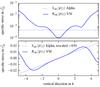Fig. 2 Specific stress tensor (stress per density) in units of ${\mathit{c}}_{\mathrm{s}\mathrm{0}}^{\mathrm{2}}$. The solid lines represent the Reynolds stress (R) of the VSI simulation and the dotted lines refer to the viscous stress tensor (S) using α = 5 × 10-4. The Szφ line was rescaled by a factor of 650 to match to the VSI model. The dotted line in the upper panel has a constant value of 5 × 10-4.

We compare it to the viscous shear stress prescription (see Eq. (6) with ν = ν_r = ν_z) using α = 5 × 10^-4 (dotted lines), which is close to the average of the rφ-component of the specific VSI stress, 4 × 10^-4. We rescaled the zφ-component of the viscous shear stress by a factor of 650 to match the value from the VSI stress. From this large rescaling factor it is immediately clear that R_zφ is far larger than expected from an isotropic viscous shear prescription. We note that the deviation of the vertical R_rφ/ρ-profile from the constant S_rφ/ρ-profile is not important for our argument, which is why for simplicity we chose a constant α. For the angular momentum transport only the vertical average of this stress component plays a role. In our case, the very large zφ-component of the stress dominates the meridional flow and the influence of R_rφ is small.

4. Anisotropic viscosity of the VSI turbulence

From our numerical studies of the VSI turbulence, in particular the vertical component of the Reynolds stress tensor, we can infer that the turbulence is non-isotropic. Even though we have integrated the hydrodynamical equations using spherical coordinates, we calculated and display R_iφ in cylindrical coordinates because this is simpler to analyze, as we explain in the following. In our approach we investigate whether the turbulent Reynolds stresses, R, can be modeled by a viscous ansatz where R is replaced by the standard viscous stress tensor, S, with an effective turbulent eddy viscosity as introduced by Boussinesq. In cylindrical coordinates the change in angular momentum is given by the following evolution equation: 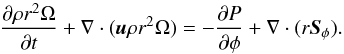$\frac{\mathit{\partial \rho }{\mathit{r}}^{\mathrm{2}}\mathrm{\Omega }}{\mathit{\partial t}}\mathrm{+}\mathrm{\nabla }\mathrm{·}\mathrm{\left(}{u}\mathit{\rho }{\mathit{r}}^{\mathrm{2}}\mathrm{\Omega }\mathrm{\right)}\mathrm{=}\mathrm{-}\frac{\mathit{\partial P}}{\mathit{\partial \phi }}\mathrm{+}\mathrm{\nabla }\mathrm{·}\mathrm{\left(}\mathit{r}{{S}}_{\mathit{\phi }}\mathrm{\right)}\mathit{.}$(5)For an axisymmetric flow, that is, when ∂/∂φ vanishes, the vector S_φ (the φ-row of the viscous stress tensor) is given by (Tassoul 1978) 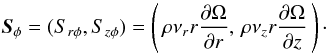${{S}}_{\mathit{\phi }}\mathrm{=}\mathrm{\left(}{\mathit{S}}_{\mathit{r\phi }}\mathit{,}{\mathit{S}}_{\mathit{z\phi }}\mathrm{\right)}\mathrm{=}\left(\hspace{0.17em}\mathit{\rho }{\mathit{\nu }}_{\mathit{r}}\mathit{r}\frac{\mathit{\partial }\mathrm{\Omega }}{\mathit{\partial r}}\mathit{,}\hspace{0.17em}\mathit{\rho }{\mathit{\nu }}_{\mathit{z}}\mathit{r}\frac{\mathit{\partial }\mathrm{\Omega }}{\mathit{\partial z}}\hspace{0.17em}\right)\mathrm{·}$(6)Axisymmetry is expected for accretion disk flows, and we found this in our simulations. In Eq. (6) we allowed for the option of an anisotropic viscosity by splitting the kinematic viscosity into two components ν_r and ν_z, where ν_r refers to the radial part, which typically is the main contribution in accretion disks in driving the angular momentum transport and mass accretion. The ν_z part connects to the vertical variation of the angular velocity Ω and has commonly been assumed to be on the same order as ν_r. Indeed, using ν_z = ν_r and performing viscous axisymmetric, two-dimensional simulations, we find the typical meridional flow field in disks with outflow in the midplane and inflow in upper layers of the disk, as shown in Fig. 1 by the curve labeled “isotropic stress”, as found in classic studies (Urpin 1984; Kley & Lin 1992). The outflow in the midplane can easily be derived by an analysis of the radial flow that can be obtained from the angular momentum equation (see also Fromang et al. 2011; Jacquet 2013). From Eq. (5) we find for the equilibrium state that 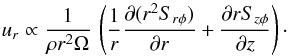${\mathit{u}}_{\mathit{r}}\mathrm{\propto }\frac{\mathrm{1}}{\mathit{\rho }{\mathit{r}}^{\mathrm{2}}\mathrm{\Omega }}\hspace{0.17em}\left(\frac{\mathrm{1}}{\mathit{r}}\frac{\mathit{\partial }\mathrm{\left(}{\mathit{r}}^{\mathrm{2}}{\mathit{S}}_{\mathit{r\phi }}\mathrm{\right)}}{\mathit{\partial r}}\mathrm{+}\frac{\mathit{\partial r}{\mathit{S}}_{\mathit{z\phi }}}{\mathit{\partial z}}\right)\mathrm{·}$(7)Expanding Eq. (3) around the midplane (small z), we find 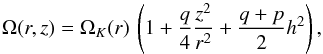$\mathrm{\Omega }\mathrm{\left(}\mathit{r,z}\mathrm{\right)}\mathrm{=}{\mathrm{\Omega }}_{\mathit{K}}\mathrm{\left(}\mathit{r}\mathrm{\right)}\hspace{0.17em}\left(\mathrm{1}\mathrm{+}\frac{\mathit{q}}{\mathrm{4}}\frac{{\mathit{z}}^{\mathrm{2}}}{{\mathit{r}}^{\mathrm{2}}}\mathrm{+}\frac{\mathit{q}\mathrm{+}\mathit{p}}{\mathrm{2}}{\mathit{h}}^{\mathrm{2}}\right)\mathit{,}$(8)where q and p are the exponents in the radial power laws of the density and temperature, respectively, and h = H/r denotes the relative scale height of the disk. Using this relation for Ω(r,z), we find 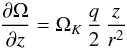$\frac{\mathit{\partial }\mathrm{\Omega }}{\mathit{\partial z}}\mathrm{=}{\mathrm{\Omega }}_{\mathit{K}}\hspace{0.17em}\frac{\mathit{q}}{\mathrm{2}}\hspace{0.17em}\frac{\mathit{z}}{{\mathit{r}}^{\mathrm{2}}}$(9)and then, neglecting terms of order z²/r²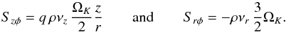${\mathit{S}}_{\mathit{z\phi }}\mathrm{=}\mathit{q}\hspace{0.17em}\mathit{\rho }{\mathit{\nu }}_{\mathit{z}}\hspace{0.17em}\frac{{\mathrm{\Omega }}_{\mathit{K}}}{\mathrm{2}}\frac{\mathit{z}}{\mathit{r}} \mathrm{and} {\mathit{S}}_{\mathit{r\phi }}\mathrm{=}\mathrm{-}\mathit{\rho }{\mathit{\nu }}_{\mathit{r}}\hspace{0.17em}\frac{\mathrm{3}}{\mathrm{2}}{\mathrm{\Omega }}_{\mathit{K}}\mathit{.}$(10)Combining this with the S_zφ relation, we find 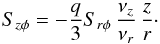${\mathit{S}}_{\mathit{z\phi }}\mathrm{=}\mathrm{-}\frac{\mathit{q}}{\mathrm{3}}{\mathit{S}}_{\mathit{r\phi }}\hspace{0.17em}\frac{{\mathit{\nu }}_{\mathit{z}}}{{\mathit{\nu }}_{\mathit{r}}}\hspace{0.17em}\frac{\mathit{z}}{\mathit{r}}\mathrm{·}$(11)This is plotted in the lower panel in Fig. 2 using ν_z = 650ν_r, which demonstrates that the linear dependence of the specific S_zφ-stress is a direct consequence of Eq. (11). From Eq. (7) we find for the relation determining the sign of u_r in the midplane the following relation: $\begin{array}{ccc}{\mathit{u}}_{\mathit{r}}\mathrm{(}\mathit{z}\mathrm{=}\mathrm{0}\mathrm{)}& \mathrm{\propto }& \left(\mathrm{2}{\mathit{S}}_{\mathit{r\phi }}\mathrm{+}\mathit{r}\frac{\mathit{\partial }{\mathit{S}}_{\mathit{r\phi }}}{\mathit{\partial r}}\mathrm{+}\mathit{r}\frac{\mathit{\partial }{\mathit{S}}_{\mathit{z\phi }}}{\mathit{\partial z}}\right)\\ & \mathrm{\propto }& \mathit{\rho }\hspace{0.17em}\left[{\mathit{\nu }}_{\mathit{r}}\left(\mathrm{-}\mathrm{3}\mathrm{-}\frac{\mathrm{3}}{\mathrm{2}}\left(\mathit{q}\mathrm{+}\mathit{p}\mathrm{+}\frac{\mathrm{3}}{\mathrm{2}}\right)\mathrm{+}\frac{\mathrm{9}}{\mathrm{4}}\right)\mathrm{+}\frac{\mathit{q}}{\mathrm{2}}{\mathit{\nu }}_{\mathit{z}}\right]\mathit{,}\end{array}$(12)where for the last step we assumed that the viscosity has an α-type behavior with $\mathit{\nu }\mathrm{~}\mathit{\alpha }{\mathit{c}}_{\mathrm{s}}^{\mathrm{2}}\mathit{/}{\mathrm{\Omega }}_{\mathit{K}}$ and ρ ∝ r^p and ${\mathit{c}}_{\mathrm{s}}^{\mathrm{2}}\mathrm{\propto }{\mathit{r}}^{\mathit{q}}$. We note that the direction of flow in the disk midplane can be influenced by the slopes (p,q) in the disk stratification (Fromang et al. 2011; Philippov & Rafikov 2017). From the above relation we find directly that for our disk with slopes q = −1 and p = −3/2 that ${\mathit{u}}_{\mathit{r}}\mathrm{(}\mathit{z}\mathrm{=}\mathrm{0}\mathrm{)}\mathrm{\propto }\left[\frac{\mathrm{3}}{\mathrm{2}}{\mathit{\alpha }}_{\mathit{r}}\mathrm{-}{\mathit{\alpha }}_{\mathit{z}}\right]\mathit{.}$(13)For isotropic turbulence with α_r = α_z we therefore have outflow in the disk midplane. For the turning point we find that α_z must be larger than 1.5α_r. Upon increasing α_z over α_r, the midplane radial velocity becomes more and more negative, and the entire vertical flow profile eventually reverses. In our numerical simulations of viscous disks using different values for ν_z we could indeed find the observed flow reversal for moderate values of ν_z/ν_r. By increasing ν_z further, we found that the VSI turbulence can be modeled by an anisotropic eddy viscosity with ν_z over two magnitudes larger than ν_r (650 for our chosen parameter, as shown in Fig. 2).

In performing the comparison simulations, we initially tried to use the same spherical coordinate system that we used for the turbulent VSI simulations by just increasing ν_θ over ν_R in the corresponding components of the stress tensor in spherical coordinates. However, this did not lead to the expected results, in particular, the inversion of the parabola of u_r(z). The results displayed in Fig. 1 were therefore obtained using a cylindrical coordinate system. Because the usage of a spherical coordinate system is beneficial in disk simulations, the equations need to be transformed from r,z to R,θ.

This means we need to transform the viscous part, ∇·(rS_φ), to spherical coordinates. The transformation equations are $\mathit{r}\mathrm{=}\mathit{R}\sin \mathit{\theta } \mathrm{and} \mathit{z}\mathrm{=}\mathit{R}\cos \mathit{\theta ,}$(14)and the components of the stress tensor transform according to 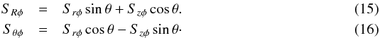$\begin{array}{ccc}{\mathit{S}}_{\mathit{R\phi }}& \mathrm{=}& {\mathit{S}}_{\mathit{r\phi }}\sin \mathit{\theta }\mathrm{+}{\mathit{S}}_{\mathit{z\phi }}\cos \mathit{\theta }\mathit{.}\\ {\mathit{S}}_{\mathit{\theta \phi }}& \mathrm{=}& \end{array}$The derivatives of Ω transform then as $\begin{array}{ccc}\frac{\mathit{\partial }\mathrm{\Omega }}{\mathit{\partial r}}& \mathrm{=}& \sin \mathit{\theta }\frac{\mathit{\partial }\mathrm{\Omega }}{\mathit{\partial R}}\hspace{0.17em}\mathrm{+}\hspace{0.17em}\frac{\cos \mathit{\theta }}{\mathit{R}}\frac{\mathit{\partial }\mathrm{\Omega }}{\mathit{\partial \theta }}\\ \frac{\mathit{\partial }\mathrm{\Omega }}{\mathit{\partial z}}& \mathrm{=}& \cos \mathit{\theta }\frac{\mathit{\partial }\mathrm{\Omega }}{\mathit{\partial R}}\hspace{0.17em}\mathrm{-}\hspace{0.17em}\frac{\sin \mathit{\theta }}{\mathit{R}}\frac{\mathit{\partial }\mathrm{\Omega }}{\mathit{\partial \theta }}\mathit{.}\end{array}$Using Eq. (6) in Eqs. (15) and (16) and substituting this into Eqs. (17) and (18), we obtain for the stress tensor components in spherical coordinates $\begin{array}{ccc}{\mathit{S}}_{\mathit{R\phi }}& \mathrm{=}& \mathit{\rho R}\sin \mathit{\theta }\left[\mathrm{(}{\mathit{\nu }}_{\mathit{r}}{\sin }^{\mathrm{2}}\mathit{\theta }\mathrm{+}{\mathit{\nu }}_{\mathit{z}}{\cos }^{\mathrm{2}}{\mathit{\theta }}^{\mathrm{)}}\frac{\mathit{\partial }\mathrm{\Omega }}{\mathit{\partial R}}\mathrm{+}\mathrm{(}{\mathit{\nu }}_{\mathit{r}}\mathrm{-}{\mathit{\nu }}_{\mathit{z}}\mathrm{)}\frac{\cos \mathit{\theta }\sin \mathit{\theta }}{\mathit{R}}\frac{\mathit{\partial }\mathrm{\Omega }}{\mathit{\partial \theta }}\hspace{0.17em}\right]\\ {\mathit{S}}_{\mathit{\theta \phi }}& \mathrm{=}& \end{array}$As can be inferred from these equations, the relatively simple anisotropic relation in cylindrical coordinates leads to complex coupled equations in spherical coordinates with cross terms in the derivatives for Ω. For the isotropic case we can set ν_r = ν_z = ν and obtain the standard relations for the stress tensor components in Rθ-coordinates (Tassoul 1978). Now it becomes clear why merely increasing the θ part of the viscosity in Rθ-coordinates did not yield the correct answer when compared to the VSI case. Using the full viscosity terms as described in Eqs. (19) and (20) in the numerical simulations yields the correct behavior. However, this comes with a serious drawback because in this case the numerical integration required much smaller time steps for numerical stability than the cylindrical simulation with the same viscosity coefficients. Performing multidimensional simulations of viscous disks mimicking the non-isotropic behavior of the VSI turbulence in Rθ-coordinates therefore requires a considerable numerical effort. One solution

to this problem may be the usage of an implicit solver for the viscous terms.

5. Conclusions

From direct three-dimensional simulations of locally isothermal accretion disks we observed that the eddies introduced by the VSI generate stresses that are strongly anisotropic. Specifically, we found that the vertical zφ-component of the Reynolds stress is enhanced by a factor of 650 over the standard rφ-part. By performing viscous disk simulations using a non-isotropic viscosity with α_z highly enlarged over α_r, we could obtain the same flow reversal as seen in the VSI disk, which verifies the non-isotropy of the viscosity. Hence, the reversal of the radial flow profile compared to the usual α-model is a clear consequence of the anisotropy. This will have an effect on the dust migration processes (Stoll & Kley 2016) that need to be contrasted to the outward drift in the midplane viscous models (Takeuchi & Lin 2002). From this we can conclude that we need to be careful with turbulence models imposed on accretions disks when we adopt viscous models to describe them.

The meridional circulation of MRI-turbulent disks has been analyzed by Fromang et al. (2011), who found a similar mean flow dynamics in the disk but did not attribute it to a non-isotropic turbulence (with large S_zφ) but rather to a radial variation in the magnitude of the viscosity. However, their turbulent R_zφ profile (in Fig. 5) indicates that it may be enhanced over the standard viscous value as well, which could also be a reason for the flow reversal.

Even though the analysis is performed for simplicity for a locally isothermal disk, our results are quite general as simulations for fully radiative disks show the same behavior although they have different radial and vertical temperature profiles. For this purpose, we reanalyzed our radiative simulations in Stoll & Kley (2016) and found a similar anisotropy. Concerning numerical resolution, simulations with double resolution show the same results as shown in Fig. 1. Nevertheless, further exploration needs to be done in order to check how the anisotropy factor varies for different disk parameters and to explore the possibility of anisotropic stresses in MRI models.

Acknowledgments

Moritz Stoll received financial support from the Landesgraduiertenförderung of the state of Baden-Württemberg and through the German Research Foundation (DFG) grant KL 650/16. G. Picogna acknowledges the support through DFG-grant KL 650/21 within the collaborative research program “The first 10 Million Years of the Solar System”. Some simulations were performed on the bwGRiD cluster in Tübingen, funded by the state of Baden-Württemberg and the DFG. We thank Roman Rafikov for providing us with a preprint and very useful discussions.

References

All Tables

All Figures

Fig. 1 Radial velocity averaged over 50 orbits. We compare the disk with alpha-viscosity (α = 5 × 10-4, blue curve) to a disk with active VSI (red curve), a disk with active VSI and doubled resolution (red dotted curve) and a viscous disk with anisotropic stress similar to the VSI disk (green curve, details see Sect. 4). For the turbulent disk the velocity has been azimuthally averaged. The profile shown is in units of sound speed cs0 and at r = r0. The viscous case has been rescaled to better visualize the difference.

In the text

Fig. 2 Specific stress tensor (stress per density) in units of ${\mathit{c}}_{\mathrm{s}\mathrm{0}}^{\mathrm{2}}$. The solid lines represent the Reynolds stress (R) of the VSI simulation and the dotted lines refer to the viscous stress tensor (S) using α = 5 × 10-4. The Szφ line was rescaled by a factor of 650 to match to the VSI model. The dotted line in the upper panel has a constant value of 5 × 10-4.

In the text

References

- Balbus, S. A., & Hawley, J. F. 1998, Rev. Mod. Phys., 70, 1 [Google Scholar]
- Balbus, S. A., & Papaloizou, J. C. B. 1999, ApJ, 521, 650 [NASA ADS] [CrossRef] [Google Scholar]
- de Val-Borro, M., Edgar, R. G., Artymowicz, P., et al. 2006, MNRAS, 370, 529 [NASA ADS] [CrossRef] [Google Scholar]
- Fromang, S., Lyra, W., & Masset, F. 2011, A&A, 534, A107 [NASA ADS] [CrossRef] [EDP Sciences] [Google Scholar]
- Gammie, C. F. 1996, ApJ, 457, 355 [NASA ADS] [CrossRef] [Google Scholar]
- Jacquet, E. 2013, A&A, 551, A75 [NASA ADS] [CrossRef] [EDP Sciences] [Google Scholar]
- Kley, W., & Lin, D. N. C. 1992, ApJ, 397, 600 [NASA ADS] [CrossRef] [Google Scholar]
- Mignone, A., Bodo, G., Massaglia, S., et al. 2007, ApJS, 170, 228 [Google Scholar]
- Nelson, R. P., Gressel, O., & Umurhan, O. M. 2013, MNRAS, 435, 2610 [NASA ADS] [CrossRef] [Google Scholar]
- Philippov, A. A., & Rafikov, R. R. 2017, ApJ, submitted [arXiv:1701.01912] [Google Scholar]
- Shakura, N. I., & Sunyaev, R. A. 1973, A&A, 24, 337 [NASA ADS] [Google Scholar]
- Stoll, M. H. R., & Kley, W. 2014, A&A, 572, A77 [NASA ADS] [CrossRef] [EDP Sciences] [Google Scholar]
- Stoll, M. H. R., & Kley, W. 2016, A&A, 594, A57 [NASA ADS] [CrossRef] [EDP Sciences] [Google Scholar]
- Takeuchi, T., & Lin, D. N. C. 2002, ApJ, 581, 1344 [NASA ADS] [CrossRef] [Google Scholar]
- Tassoul, J.-L. 1978, Theory of rotating stars (Princeton: University Press) [Google Scholar]
- Urpin, V. A. 1984, Sov. Astron., 28, 50 [NASA ADS] [Google Scholar]