| Issue |
A&A
Volume 598, February 2017
|
|
|---|---|---|
| Article Number | A117 | |
| Number of page(s) | 7 | |
| Section | The Sun | |
| DOI | https://doi.org/10.1051/0004-6361/201630033 | |
| Published online | 10 February 2017 | |
Analytic solution of an oscillatory migratory α2 stellar dynamo
1 Nordita, KTH Royal Institute of Technology and Stockholm University, 10691 Stockholm, Sweden
e-mail: This email address is being protected from spambots. You need JavaScript enabled to view it.
2 JILA and Department of Astrophysical and Planetary Sciences, University of Colorado, Boulder, CO 80303, USA
3 Laboratory for Atmospheric and Space Physics, University of Colorado, Boulder, CO 80303, USA
4 Department of Astronomy, Stockholm University, 10691 Stockholm, Sweden
Received: 8 November 2016
Accepted: 1 December 2016
Abstract
Context. Analytic solutions of the mean-field induction equation predict a nonoscillatory dynamo for homogeneous helical turbulence or constant α effect in unbounded or periodic domains. Oscillatory dynamos are generally thought impossible for constant α.
Aims. We present an analytic solution for a one-dimensional bounded domain resulting in oscillatory solutions for constant α, but different (Dirichlet and von Neumann or perfect conductor and vacuum) boundary conditions on the two boundaries.
Methods. We solve a second order complex equation and superimpose two independent solutions to obey both boundary conditions.
Results. The solution has time-independent energy density. On one end where the function value vanishes, the second derivative is finite, which would not be correctly reproduced with sine-like expansion functions where a node coincides with an inflection point. The field always migrates away from the perfect conductor boundary toward the vacuum boundary, independently of the sign of α.
Conclusions. The obtained solution may serve as a benchmark for numerical dynamo experiments and as a pedagogical illustration that oscillatory migratory dynamos are possible with constant α.
Key words: dynamo / magnetohydrodynamics (MHD) / magnetic fields / Sun: magnetic fields / stars: magnetic field
© ESO, 2017
1. Introduction
The magnetic fields in stars and galaxies are believed to be generated and maintained by large-scale dynamos that convert kinetic energy into magnetic energy through an inverse cascade (Pouquet et al. 1976). With the development of mean-field theory (Parker 1955; Steenbeck et al. 1966), this complicated three-dimensional process became amenable to simpler analytic and numerical treatments in one and two dimensions.
The best known mean-field effect is the α effect, which emerges from the parameterization of the turbulent electromotive force in terms of the mean field in the form 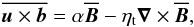 (1)where u and b are the fluctuating velocity and magnetic fields, overbars denote averaging, and
  is the mean magnetic field. Here, α quantifies the α effect and ηt is the turbulent magnetic diffusivity. Both are in principle functions of position, but in the present paper we treat them as constants.
The earliest model of a dynamo for the Sun goes back to Parker (1955), who considered the additional presence of differential rotation, which is referred to as the Ω affect. In the presence of both α and Ω effects, there are self-excited oscillatory plain wave solutions in unbounded domains. They take the form of traveling waves (Parker 1955). Specifically, if α is positive in the north and negative in the south, and the differential rotation has a negative radial gradient, waves are traveling equatorward, providing thus an explanation for the shape of Maunder’s butterfly diagram (Maunder 1904). The first global axisymmetric two-dimensional models of such dynamos go back to the seminal work of Steenbeck & Krause (1969a). These dynamos are referred to as αΩ dynamos.
In the absence of differential rotation, a plain wave solution ansatz leads to non-oscillatory dynamos if α exceeds a certain threshold (α>ηtk, where k is the wavenumber). Such dynamos are referred to as α2 dynamos. The dynamo of the Earth is believed to be an example of an α2 dynamo, because shear is expected to be weak. Axisymmetric models of dynamos of this type where presented by Steenbeck & Krause (1969b). The non-oscillatory property of such dynamos is consistent with the noncyclic nature of the Earth’s magnetic field. In galaxies, on the other hand, shear is important, so they are examples of αΩ dynamos. However, asymptotic solutions have shown that such dynamos are non-oscillatory owing to the flat geometry in which such dynamos are embedded (Vainshtein & Ruzmaikin 1971).
Numerical investigations of α2 dynamos revealed only nonoscillatory solutions (Rädler 1980), until Shukurov et al. (1985) found that, under certain conditions, oscillatory solutions are here possible, too. They associated this with the non-selfadjointness of the problem. In fact, the possibility of oscillatory solutions to an α2 dynamo was already mentioned earlier by Ruzmaikin et al. (1980) in a study of disk dynamos with a strongly localized α effect. In 1987, there appeared two back-to-back papers that demonstrated conclusively that α2 dynamos can in principle be oscillatory provided the α effect is non-constant (Baryshnikova & Shukurov 1987; Rädler & Bräuer 1987). This possibility remained mainly an academic curiosity without real astrophysical interest at the time.
In subsequent years, attention was drawn to the possibility that global dynamos with radially dependent α can exhibit oscillatory solutions (Stefani & Gerbeth 2003). Meanwhile, direct numerical simulations of helically forced turbulence have shown a strong similarity between α effect dynamos and turbulent three-dimensional dynamos with fluctuating magnetic fields and nonvanishing mean fields. These dynamos turned out to be equivalent to those predicted from α-effect dynamos (Brandenburg 2001). Mitra et al. (2009) applied such dynamos to spherical wedges with helically forced turbulence. When the helicity of the forcing was assumed such that it changes sign about the equator, Mitra et al. (2010) found oscillatory solutions with equatorward migration similar to what occurs in the Sun. Käpylä et al. (2013) argued that such an effect can explain the equatorward migration in their spherical wedge-geometry dynamos, even though shear was still present and, as it turned out later, responsible for an αΩ-type dynamo in this case (Warnecke et al. 2014). In other simulations, however, the argument in favor of an α2 dynamo could still be supported (Masada & Sano 2014).
Corresponding mean-field solutions were presented by Brandenburg et al. (2009) for dynamos in Cartesian geometry with α profiles proportional to z. Cole et al. (2016) showed that such dynamos are not necessarily expected to operate in spherical shells that extend all the way to the poles, unless the turbulent magnetic diffusivity becomes small at high latitudes. The true applicability of such α2 dynamos to stars remains therefore questionable. Nevertheless, such dynamos are gaining in importance in view of the many numerical studies of turbulent dynamos, in which the helicity profile is non-uniform (Mitra et al. 2014; Jabbari et al. 2016) and/or the boundary conditions on the two sides of the domain are different (Jabbari et al. 2017). This has led to the possibility that oscillatory α2 dynamos might actually be possible for constant α, provided the boundary conditions are indeed different and the two sides. If this is the case, it should be possible to construct exact analytical solutions of such an oscillatory migratory α2 dynamos. The purpose of the present paper is therefore to present such a solution. The fact that such a solution can be obtained analytically is significant not only as a benchmark for numerical studies, but also as a clear textbook-style demonstration of oscillatory α2 dynamos.
2. Statement of the problem
The equation for an α2 dynamo with total (sum of microphysical and turbulent) magnetic diffusivity, ηT = η + ηt, is given by 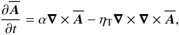 (2)where
  is the mean magnetic vector potential in the Weyl gauge, and the mean magnetic field is
  . We nondimensionalize by measuring lengths in units of
  , where k1 is the wavenumber of the most slowly decaying mode, and time is measured in units of the turbulent-diffusive time,
  . Velocities are measured in units of ηTk1, so in the following we denote by α the nondimensional α effect, α/ηTk1. We now consider a one-dimensional domain, so the governing equations are,
 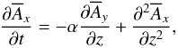 (3)
(3)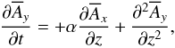 (4)and
  . In the following, all quantities are dimensionless. We consider perfect conductor boundary condition on one side of the domain (z = 0). This means that the electric field in the xy plane vanishes on the boundary. Owing to the use of the Weyl gauge, the electrostatic potential gradient is absent in Eq. (2), so the perfect conductor condition implies that
  .
.
On the other side of the domain, we assume a vacuum boundary condition. For our one-dimensional domain, this means that  (Ruzmaikin et al. 1988), which corresponds to
  . The most slowly decaying mode is a quarter sine wave, that is,
  or
or  are proportional to sinz in 0 ≤ z ≤ π/ 2 (Brandenburg et al. 2009).
3. Complex notation and integral constraints
The basic approach used here is similar to that in other problems with constant coefficients and in finite domains with boundary conditions, such as the no-slip condition in Rayleigh-Bénard convection (Chandrasekhar 1961) or the pole-equator boundary conditions in αΩ dynamos (Parker 1971). Unlike convection, which is non-oscillatory at onset, we allow here for oscillatory solutions. Furthermore, we combine Eqs. (3) and (4) into a single equation for the complex variable  (5)Thus, Eqs. (3) and (4) can be written as
  (6)We now assume the solution to be of the form
  (7)where
  obeys the ordinary differential equation
  (8)where primes denote z derivatives. The boundary conditions are
 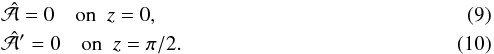 In general, ω can be complex, but since we are here interested in marginally excited dynamos, we restrict ourselves in the following to ω being real.
We now also assume that α is constant. In that case, oscillatory solutions were previously thought impossible (Rädler & Bräuer 1987). Analogously to their approach, we multiply Eq. (8) by  , where the asterisk denotes complex conjugation, and integrate by parts. Using Eqs. (9) and (10), we obtain
 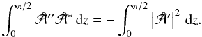 (11)Furthermore,
  , so
, so 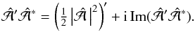 (12)Equation (8) yields altogether four terms, two of which are real and the other two imaginary. We obtain two integral constraints
 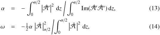 where
where  denotes the value of
  on the second boundary at z = π/ 2. This implies that αω ≤ 0 (negative frequencies for positive α) and ω ≠ 0 if
  and α ≠ 0.
Similar integral constraints can also be formulated for the complex magnetic field,  . Unfortunately, the perfect conductor boundary condition,
  , is more cumbersome. Instead, one could formulate the problem for an artificially modified boundary condition,
  on z = 0. Together with the condition
  on z = π/ 2, the problem for
  becomes equivalent to that for . In either case, the integral constraints are analogous to those of Rädler & Bräuer (1987); see Appendix A for details.
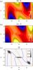 |
Fig. 1 Plots of a) real, b) imaginary, and c) absolute parts of D(α,ω). In a) and b), the zero lines are marked in white, while in c) those of ReD are dotted blue and those of ImD are solid red. |
4. The solution
Given that Eq. (8) has constant coefficients, it has solutions proportional to 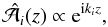 (15)where the index i denotes one of two independent solutions. The ki are in general complex and obey the characteristic equation
 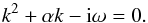 (16)It has two solutions,
 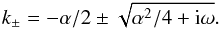 (17)To satisfy the boundary conditions (9) and (10), we write the solution as a superposition of eik+z and eik−z. Equation (9) is readily satisfied by writing
  (18)where we have ignored the possibility of an arbitrary (complex) constant in front of
  . To satisfy Eq. (10), we now require that
  (19)vanishes. The existence of solutions to D(α,ω) = 0 is demonstrated by looking at a contour plot of | D |; see Fig. 1, where we also plot separately the real and imaginary parts of D. We see two zeroes in D(α,ω), which is confirmed by the crossing of the lines where ReD and ImD vanish. (At α = ω = 0, there is no such crossing, so D(0) is not a solution.) The transcendental equation relating α to ω can be written in more explicit form as
  (20)To find solutions to D(α,ω) = 0, it is convenient to introduce the complex variable
  (21)We seek solutions to D(Z) = 0 via complex interpolation,
  (22)where subscripts 0 and −1 refer to the current and previous iteration. This yields the first critical value as
  (23)with the corresponding complex wavenumbers
  The wavenumbers k+ and k− obey the relation
  (26)which follows from Eqs. (9) and (18). The critical values of α and ω were first obtained by Jabbari et al. (2017) using explicit time integration.
Additional solutions exist in the second and fourth quadrant of the αω plane; see Fig. 2. They are all oscillatory, in agreement with the integral constraints; see Eqs. (13) and (14) and Table 1. However, those higher modes would generally be unstable in a nonlinear calculation and therefore only of limited interest (Brandenburg et al. 1989).
Critical values of α and ω for the higher modes.
The solution is now completely described by the value of Z∗. It is convenient to write the solution in the form  (27)where rA(z) and φA(z) are amplitude and phase of . In view of computing magnetic field and current density, we also define
  (28)and
  (29)respectively. In Fig. 3 we plot the moduli and phases of , , and
  . Note that rA(0) = 0, as required by Eq. (9), and
  , as required by Eq. (10). In general, however,
  . The derivative of the phase is an “effective” wavenumber,
  , and determines the z-dependent phase speed
  , which is positive for positive α, so the wave moves in the positive z direction.
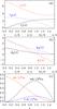 |
Fig. 3 a) Moduli and b) phases of |
In Fig. 3c we plot the magnetic and current helicity densities, as well as the z component of the Lorentz force,  (30)normalized by
  and
and  for the first, and second and third quantities, respectively. The Lorentz force has a maximum at z = 0.937, which is also the point where the magnetic helicity density in the Weyl gauge has a maximum. The current helicity density, however, has a maximum at z = 0. The ratio between the integrals of the two helicity densities is
 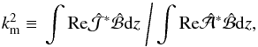 (31)where km denotes the wavenumber of the mean field; see Eq. (25) of Blackman & Brandenburg (2002). For α2 dynamos in periodic domains, one finds km/k1 = 1, but here we obtain km/k1 ≈ 2.253027. Interestingly, this is also the value of the magnetic Taylor microscale wavenumber of the mean field, kT, defined through
 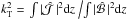 , i.e., kT = km. Finally, for the fractional current helicity of the mean field (Blackman & Brandenburg 2002),
 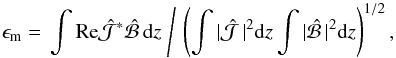 (32)we find ϵm ≈ 0.883315, which is close to the value ϵm = 1 for α2 dynamos in periodic domains (Blackman & Brandenburg 2002).
To plot butterfly diagrams of  and
and  , we can now write the fully time-dependent magnetic field as
![Mathematical equation: \begin{equation} \begin{array}{llll} \meanB_x(z,t)=r_B(z) \cos[\phi_B(z)-\omega t],\\ \meanB_y(z,t)=r_B(z) \sin[\phi_B(z)-\omega t]. \end{array} \end{equation}](/articles/aa/full_html/2017/02/aa30033-16/aa30033-16-eq126.png) (33)This also demonstrates that the magnetic energy density,
(33)This also demonstrates that the magnetic energy density, 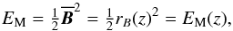 (34)is independent of time and only a function of z. In fact, the magnetic and current helicity densities, as well as the z component of the Lorentz force, all shown in Fig. 3c, are also independent of time. The results for
  and
and  are shown in Fig. 4, where z increases downward so as to facilitate comparison with Fig. 2 of Brandenburg et al. (2009), who adopted a perfect conductor boundary condition at high latitudes and a vacuum condition at the equator. In their case, however, α was non-constant and vanishing on the equator.
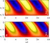 |
Fig. 4 Butterfly diagrams for |
5. Discussion
The graphs of the solutions obtained here look rather simple, but would have been impossible to guess based on previous experience with one-dimensional dynamos with vacuum field conditions on both ends of the domain. The field components of those dynamos are proportional to cosz eiz. Such dynamos have been studied extensively in connection with demonstrating the asymptotically equal growth rates of even and odd dynamo modes (Brandenburg et al. 1989), the behavior of dynamos in the highly nonlinear regime (Meinel & Brandenburg 1990), and the effects of magnetic helicity fluxes (Brandenburg & Dobler 2001). Thus, one might have expected that the solution to the present problem could have been expanded in terms of sine functions proportional to sin (2n + 1)z with integers n ≥ 0. Such functions obey the boundary conditions of on z = 0 and π/ 2. However, one sees immediately that such a solution for would imply that has terms proportional to cos (2n + 1)z, which would then violate the boundary conditions on on both boundaries; see Appendix B for details. This is indeed be a problem for spectral codes that employ sine or cosine transforms; see Vasil et al. (2008a,b) for detailed studies and alternative approaches. It can also be a problem for codes that use symmetry conditions to populate the ghost zones outside the computational mesh, as is done by default in the Pencil Code1. This highlights once more the significance of having an independent and analytic solution of such a dynamo. To demonstrate this, we summarize in Table 2 the values of α and | ω | for a marginally excited dynamo obtained by using either one-sided (1s) finite difference formulae on the boundaries or symmetry/antisymmetry (s) conditions (Brandenburg 2003) for different meshpoint numbers Nmesh. The 1s scheme does not restrict the second derivative and is found to be slightly better than the s scheme.
Values of α and | ω | using one-sided (1s) finite difference formulae on the boundaries and symmetry/antisymmetry (s) conditions for different meshpoint numbers Nmesh.
We have here also been able to find higher order modes. They all lie in the same two quadrants in the αω plane. Thus, for positive α, we always have ω< 0. When determining ω empirically from the period of the oscillation, it would not have a definite sign, although the sign has implications for the phase speed. For αΩ dynamos with differential rotation gradient Ω′ in periodic domains with real wavenumber k, self-excited solutions exist only when sgn [(kαΩ′)ω] > 0; see Appendix C and Table 3 of Brandenburg & Subramanian (2005). However, unlike αΩ dynamos, where both migration directions are possible, depending just on sgn (αΩ′), for oscillatory α2 dynamos, the migration direction is always away from the (perfect) conductor toward the vacuum. This agrees with earlier findings for oscillatory α2 dynamos with nonuniform α profiles (Brandenburg et al. 2009).
In the context of oscillatory αΩ dynamos, boundary conditions have long been known to introduce behaviors that are not obtained for infinite domains (Parker 1971). The antisymmetry condition at the equator was found to play the role of an absorbing boundary that led to localized wall modes (Worledge et al. 1997; Tobias et al. 1997). Subsequent work using complex amplitude equations for the envelope of a wave train demonstrated that boundary conditions can play a decisive role in determining the migration direction of traveling waves (Tobias et al. 1998). They emphasized that the traveling wave behavior is linked to the symmetry-breaking in the mean-field dynamo equations. This rather general result could explain the migration direction of the α2 dynamo studied here. The symmetry breaking, which occurs here through the boundary conditions, might also be responsible for the occurrence of an oscillatory mode rather than the non-selfadjointness mentioned in the introduction (Shukurov et al. 1985).
6. Conclusions
The present work has shown that α2 dynamos with constant α can have oscillatory solutions provided the boundary conditions on the two ends of the domain are different. It is possible to construct a one-dimensional analytic solution characterized by a complex function , which obeys Dirichlet and von Neumann boundary conditions on the two ends of the domain. The solution has been obtained as a superposition of two harmonic functions with complex wavenumbers. In principle, we could have solved the problem directly for , but the boundary condition on z = 0, namely , would be more complicated. Integral constraints on  would then be harder to impose, unless one changed the perfect conductor boundary condition to . In that case, the problem becomes equivalent to the one considered here if we replace
  . In this connection, it should be noted that the very assumption of a finite α effect on a perfect conductor boundary, while mathematically sound, is physically not strictly realistic, because an impenetrable boundary would necessarily make α anisotropic such that its tangential components would vanish (Rädler 1982). Nevertheless, various DNS with helically forced turbulence extending all the way to the walls confirm the presence of oscillatory migratory solutions (Mitra et al. 2010; Warnecke et al. 2011; Jabbari et al. 2017).
Owing to our restriction to Cartesian geometry, the main application of this model lies in the comparison with other numerical solutions in the same geometry (see, e.g., Jabbari et al. 2017). The present solution demonstrates clearly that a model with constant α is possible and has time-independent magnetic energy density. Thus, when looking only at the rms value of the magnetic field or the volume-integrated energy, one will not notice the presence of an oscillatory solution.
When the α2 dynamo is applied to a star, α would have the opposite sign on the other side of the equator (here for z>π/ 2) and would then be described by a step function. In that case, the field could be either symmetric or antisymmetric about the equator. Earlier work with a linear α profile suggests that the antisymmetric solution is more easily excited (Brandenburg et al. 2009; Cole et al. 2016). Such solutions would have a discontinuity in the derivative of the current density at the equator. More dramatic, however, would be the case of symmetric solutions when a vacuum or vertical field condition is assumed on the outer boundary, because in that case the current density itself would be discontinuous at the equator. Interestingly, the critical values of α are the same in both cases. While a step function profile of α is artificial, it does pose a simple benchmark for numerical schemes. The analytic solution presented here applies also to this case. This solution may also serve as a pedagogical illustration that oscillatory migratory dynamos with constant α are possible.
Acknowledgments
I thank Ben Brown, Matthias Rheinhardt, and an anonymous referee for useful remarks. This work was supported in part by the Swedish Research Council grant No. 2012-5797, and the Research Council of Norway under the FRINATEK grant 231444. This work utilized the Janus supercomputer, which is supported by the National Science Foundation (award number CNS-0821794), the University of Colorado Boulder, the University of Colorado Denver, and the National Center for Atmospheric Research. The Janus supercomputer is operated by the University of Colorado Boulder.
References
- Baryshnikova, Y., & Shukurov, A. M. 1987, Astron. Nachr., 308, 89 [NASA ADS] [CrossRef] [Google Scholar]
- Blackman, E. G., & Brandenburg, A. 2002, ApJ, 579, 359 [Google Scholar]
- Brandenburg, A. 2001, ApJ, 550, 824 [NASA ADS] [CrossRef] [Google Scholar]
- Brandenburg, A. 2003, in Advances in nonlinear dynamos eds. A. Ferriz-Mas, & M. Núñez (London and New York: Taylor & Francis), The Fluid Mechanics of Astrophysics and Geophysics, Chap. 9, 269 [Google Scholar]
- Brandenburg, A., & Dobler, W. 2001, A&A, 369, 329 [NASA ADS] [CrossRef] [EDP Sciences] [Google Scholar]
- Brandenburg, A., & Subramanian, K. 2005, Phys. Rep., 417, 1 [NASA ADS] [CrossRef] [Google Scholar]
- Brandenburg, A., Krause, F., Meinel, R., Moss, D., & Tuominen, I. 1989, A&A, 213, 411 [NASA ADS] [Google Scholar]
- Brandenburg, A., Nordlund, Å., Stein, R. F., & Torkelsson, U. 1995, ApJ, 446, 741 [NASA ADS] [CrossRef] [Google Scholar]
- Brandenburg, A., Candelaresi, S., & Chatterjee, P. 2009, MNRAS, 398, 1414 [NASA ADS] [CrossRef] [Google Scholar]
- Candelaresi, S., Hubbard, A., Brandenburg, A., & Mitra, D. 2011, Phys. Plasmas, 18, 012903 [NASA ADS] [CrossRef] [Google Scholar]
- Chandrasekhar, S. 1961, in Hydrodynamic and Hydromagnetic Stability (New York: Dover Publications), Sect. 15, 37 [Google Scholar]
- Cole, E., Brandenburg, A., Käpylä, P. J., & Käpylä, M. J. 2016, A&A, 593, A134 [NASA ADS] [CrossRef] [EDP Sciences] [Google Scholar]
- Jabbari, S., Brandenburg, A., Mitra, D., Kleeorin, N., & Rogachevskii, I. 2016, MNRAS, 459, 4046 [NASA ADS] [CrossRef] [Google Scholar]
- Jabbari, S., Brandenburg, A., Kleeorin, N., & Rogachevskii, I. 2017, MNRAS, in press, DOI: 10.1093/mnras/stx148 [Google Scholar]
- Käpylä, P. J., Mantere, M. J., Cole, E., Warnecke, J., & Brandenburg, A. 2013, ApJ, 778, 41 [NASA ADS] [CrossRef] [Google Scholar]
- Masada, Y., & Sano, T. 2014, ApJ, 794, L6 [NASA ADS] [CrossRef] [Google Scholar]
- Maunder, E. W. 1904, MNRAS, 64, 747 [NASA ADS] [Google Scholar]
- Meinel, R., & Brandenburg, A. 1990, A&A, 238, 369 [NASA ADS] [Google Scholar]
- Mitra, D., Tavakol, R., Brandenburg, A., & Moss, D. 2009, ApJ, 697, 923 [NASA ADS] [CrossRef] [Google Scholar]
- Mitra, D., Tavakol, R., Käpylä, P. J., & Brandenburg, A. 2010, ApJ, 719, L1 [NASA ADS] [CrossRef] [Google Scholar]
- Mitra, D., Brandenburg, A., Kleeorin, N., & Rogachevskii, I. 2014, MNRAS, 445, 761 [NASA ADS] [CrossRef] [Google Scholar]
- Parker, E. N. 1955, ApJ, 122, 293 [NASA ADS] [CrossRef] [Google Scholar]
- Parker, E. N. 1971, ApJ, 164, 491 [NASA ADS] [CrossRef] [Google Scholar]
- Pouquet, A., Frisch, U., & Léorat, J. 1976, J. Fluid Mech., 77, 321 [NASA ADS] [CrossRef] [Google Scholar]
- Rädler, K.-H. 1980, A&A, 301, 101 [Google Scholar]
- Rädler, K.-H. 1982, Geophys. Astrophys. Fluid Dyn., 20, 191 [NASA ADS] [CrossRef] [Google Scholar]
- Rädler, K.-H., & Bräuer, H.-J. 1987, Astron. Nachr., 308, 101 [NASA ADS] [CrossRef] [Google Scholar]
- Ruzmaikin, A. A., Sokolov, D. D., & Shukurov, A. M. 1980, Magnetohydrodyn., 16, 15 [Google Scholar]
- Ruzmaikin, A. A., Sokoloff, D. D., & Shukurov, A. M. 1988, Magnetic Fields of Galaxies (Dordrecht: Kluwer) [Google Scholar]
- Shukurov, A. M., Sokolov, D. D., & Ruzmaikin, A. A. 1985, Magnetohydrodyn., 3, 6 [Google Scholar]
- ; translated from 1985, Magnitnaia Gidrodinamika, 3, 9 [Google Scholar]
- Steenbeck, M., & Krause, F. 1969a, Astron. Nachr., 291, 49 [NASA ADS] [CrossRef] [Google Scholar]
- Steenbeck, M., & Krause, F. 1969b, Astron. Nachr., 291, 271 [Google Scholar]
- Steenbeck, M., Krause, F., & Rädler, K.-H. 1966, Z. Naturforsch., 21a, 369 [Google Scholar]
- Stefani, F., & Gerbeth, G. 2003, Phys. Rev. E, 67, 027302 [NASA ADS] [CrossRef] [Google Scholar]
- Tobias, S. M., Proctor, M. R. E., & Knobloch, E. 1997, A&A, 318, L55 [NASA ADS] [Google Scholar]
- Tobias, S. M., Proctor, M. R. E., & Knobloch, E. 1998, Physica D, 113, 43 [NASA ADS] [CrossRef] [Google Scholar]
- Vainshtein, S. I., & Ruzmaikin, A. A. 1971, Sov. Astron., 16, 365 [NASA ADS] [Google Scholar]
- Vasil, G. M., Brummell, N. H., & Julien, K. 2008a, J. Comput. Phys., 227, 7999 [NASA ADS] [CrossRef] [Google Scholar]
- Vasil, G. M., Brummell, N. H., & Julien, K. 2008b, J. Comput. Phys., 227, 8017 [NASA ADS] [CrossRef] [Google Scholar]
- Warnecke, J., Brandenburg, A., & Mitra, D. 2011, A&A, 534, A11 [NASA ADS] [CrossRef] [EDP Sciences] [Google Scholar]
- Warnecke, J., Käpylä, P. J., Käpylä, M. J., & Brandenburg, A. 2014, ApJ, 796, L12 [NASA ADS] [CrossRef] [Google Scholar]
- Worledge, D., Knobloch, E., Tobias, S., & Proctor, M. 1997, Proc. Roy. Soc. Lond. A, 453, 119 [NASA ADS] [CrossRef] [Google Scholar]
- Yoshimura, H. 1975, ApJS, 29, 467 [NASA ADS] [CrossRef] [Google Scholar]
Appendix A: Integral constraint in multi-dimensions
The purpose of this appendix is to demonstrate the analogy between Eqs. (13) and (14) and the corresponding one of Rädler & Bräuer (1987). However, instead of assuming the dynamo region to be surrounded by vacuum and extending some of the volume integrals over all space, we adopt here perfect conductor and vertical field boundary conditions. In a multi-dimensional domain, the latter is no longer a proper vacuum condition, but it can be motivated as being a more realistic representation of stellar surface fields affected by magnetic buoyancy effects (Yoshimura 1975). Multiplying by  , the dynamo eigenvalue problem takes the form
  (A.1)Using
  (A.2)but assuming now constant α in a volume V, we obtain
  (A.3)and, as in Rädler & Bräuer (1987),
  (A.4)These equations are analogous to Eqs. (13) and (14). By comparison, Rädler & Bräuer (1987) assumed a potential field on all boundaries, so
  , where Φ is the magnetic scalar potential. Writing the integrand of the surface integral in Eq. (A.4) as ∇ × (Φ∇Φ∗) and turning the surface integral back into a volume integral, one sees that the divergence of the curl vanishes, and therefore ω = 0. However, this does not apply to our case where we have different boundary conditions on the two ends. By comparison, in one-dimensional dynamos with vacuum conditions on both ends,
  has, in a non-transient state and with the gauge
  , the same value on both boundaries, so Eq. (14) does indeed predict ω = 0.
Appendix B: Quarter sine wave expansion
In this appendix we give the results for a quarter sine wave expansion of ,  (B.1)where each element of the expansion obeys Eqs. (9) and (10). The coefficients are given by
  . We have strictly
  , although the analytic value is nonvanishing,
  . For
. For  we have
  (B.2)\newpage\noindentwhich converges extremely slowly to the analytic value obtained from Eq. (18), which is
  ; see Table B.1, where we list the first few values of
  and
and  .
.
Coefficients and .
Appendix C: Comparison with the αΩ dynamo
The purpose of this appendix is to show that for αΩ dynamos, αωΩ′k > 0 and αcΩ′ > 0, where c = ω/k is the phase speed. We assume a linear shear flow velocity  , where Ω′ is the velocity gradient. Using the advective gauge,
  (Brandenburg et al. 1995; Candelaresi et al. 2011), we have
 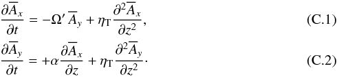 The dispersion relation is then
  (C.3)Using (2 i)1/2 = 1 + i and (− 2 i)1/2 = (1 + i)i = −1 + i, we have
 ![Mathematical equation: \appendix \setcounter{section}{3} \begin{equation} -\ii\omega\equiv-\ii kc=-\etaT k \pm \left[\ii-\sgn(k\alpha\Omega')\right] \,\left|k\alpha\Omega'/2\right|^{1/2}. \end{equation}](/articles/aa/full_html/2017/02/aa30033-16/aa30033-16-eq223.png) (C.4)For positive (negative) values of kαΩ′, only the lower (upper) sign yields marginally excited dynamos, so
(C.4)For positive (negative) values of kαΩ′, only the lower (upper) sign yields marginally excited dynamos, so  (C.5)Thus, the migration direction depends just on the sign of αΩ′, but the frequency depends also on the sign of k.
All Tables
Values of α and | ω | using one-sided (1s) finite difference formulae on the boundaries and symmetry/antisymmetry (s) conditions for different meshpoint numbers Nmesh.
All Figures
|
Fig. 1 Plots of a) real, b) imaginary, and c) absolute parts of D(α,ω). In a) and b), the zero lines are marked in white, while in c) those of ReD are dotted blue and those of ImD are solid red. |
| In the text | |
 |
Fig. 2 Similar to Fig. 1c, but for the next higher modes (+ signs). |
| In the text | |
|
Fig. 3 a) Moduli and b) phases of |
| In the text | |
|
Fig. 4 Butterfly diagrams for |
| In the text | |
Current usage metrics show cumulative count of Article Views (full-text article views including HTML views, PDF and ePub downloads, according to the available data) and Abstracts Views on Vision4Press platform.
Data correspond to usage on the plateform after 2015. The current usage metrics is available 48-96 hours after online publication and is updated daily on week days.
Initial download of the metrics may take a while.