| Issue |
A&A
Volume 598, February 2017
|
|
|---|---|---|
| Article Number | A113 | |
| Number of page(s) | 10 | |
| Section | Cosmology (including clusters of galaxies) | |
| DOI | https://doi.org/10.1051/0004-6361/201628911 | |
| Published online | 09 February 2017 | |
Cosmology with gamma-ray bursts
II. Cosmography challenges and cosmological scenarios for the accelerated Universe
1 Institute for Theoretical Physics, University of Warsaw, Pasteura 5, 02-093 Warsaw, Poland
2 Department of Astronomy, Williams College, Williamstown, MA 01267, USA
3 Dipartimento di Fisica, Università degli Studi di Napoli Federico II, Compl. Univ. Monte S. Angelo, 80126 Naples, Italy
4 INFN, Sez. di Napoli, Compl. Univ. Monte S. Angelo, Edificio 6, via Cinthia, 80126 Napoli, Italy
e-mail: This email address is being protected from spambots. You need JavaScript enabled to view it.
5 Department of Physics and Earth Sciences, University of Ferrara, Block C, via Saragat 1, 41122 Ferrara, Italy
6 Department of Physics, University of Nice Sophia Antipolis, Parc Valrose 06034, Nice Cedex 2, France
7 INAF-IASF, Sezione di Bologna, via Gobetti 101, 40129 Bologna, Italy
Received: 12 May 2016
Accepted: 17 September 2016
Abstract
Context. Explaining the accelerated expansion of the Universe is one of the fundamental challenges in physics today. Cosmography provides information about the evolution of the universe derived from measured distances, assuming only that the space time geometry is described by the Friedman-Lemaitre-Robertson-Walker metric, and adopting an approach that effectively uses only Taylor expansions of basic observables.
Aims. We perform a high-redshift analysis to constrain the cosmographic expansion up to the fifth order. It is based on the Union2 type Ia supernovae data set, the gamma-ray burst Hubble diagram, a data set of 28 independent measurements of the Hubble parameter, baryon acoustic oscillations measurements from galaxy clustering and the Lyman-α forest in the SDSS-III Baryon Oscillation Spectroscopic Survey (BOSS), and some Gaussian priors on h and ΩM.
Methods. We performed a statistical analysis and explored the probability distributions of the cosmographic parameters. By building up their regions of confidence, we maximized our likelihood function using the Markov chain Monte Carlo method.
Results. Our high-redshift analysis confirms that the expansion of the Universe currently accelerates; the estimation of the jerk parameter indicates a possible deviation from the standard ΛCDM cosmological model. Moreover, we investigate implications of our results for the reconstruction of the dark energy equation of state (EOS) by comparing the standard technique of cosmography with an alternative approach based on generalized Padé approximations of the same observables. Because these expansions converge better, is possible to improve the constraints on the cosmographic parameters and also on the dark matter EOS.
Conclusions. The estimation of the jerk and the DE parameters indicates at 1σ a possible deviation from the ΛCDM cosmological model.
Key words: dark energy / cosmological parameters / cosmology: theory
© ESO, 2017
1. Introduction
In the past dozen years a huge and diverse set of observational data revealed that the Universe is now expanding at an accelerated rate, see for instance Riess et al. (2007), Astier et al. (2006), Riess et al. (2011), Suzuki et al. (2012), Planck Collaboration XVI (2014), and Planck Collaboration XIII (2016). It is usually assumed that this accelerated expansion is caused by the so-called dark energy, a cosmic medium with unusual properties. The pressure of dark energy pde is negative, and it is related to the positive energy density of dark energy ϵde by the equation of state (EOS), pde = wϵde, where the proportionality coefficient is <−1/3. According to current estimates, about 75% of the matter energy in the Universe is in the form of dark energy, so that today the dark energy is the dominant component in the Universe. The nature of dark energy is not known. Models of dark energy proposed so far include at least a non-zero cosmological constant (in this case w = −1), a potential energy of some scalar field, effects connected with inhomogeneous distribution of matter and averaging procedures, and extended theories of gravity (an accelerated expansion can be obtained by generalizing the Einstein theory of gravity to some theory derived from a modified action with respect to the Hilbert-Einstein action: the simplest extension of General Relativity is achieved assuming that the gravitational Lagrangian is an arbitrary continuous function f(R) of the Ricci scalar R. In this case, in general, w ≠ −1 and it is not constant and depends on the redshift z. Extracting the information on the EOS of dark energy from observational data is then at the same time a fundamental problem and a challenging task. To probe the dynamical evolution of dark energy in these circumstances, we can parameterize w empirically, usually using two or more free parameters. Of all the parametrization forms of the dark energy EOS, the Chevallier-Polarski-Linder (CPL) model (Chevallier & Polarski 2001; Linder 2003), Linder (2003) is probably the most widely used, since it presents a smooth and bounded behavior for high redshifts and a manageable two-dimensional parameter space and also provides a simple and effective instrument of computations. However, it would result a in physically incomplete parametrization of dark energy if we were to take into account the inhomogeneities of the late-time Universe. Linear parametrizations of the dark energy EOS (the CPL EOS is linear in the scale factor a) are not compatible with the theory of scalar perturbations in the late Universe. Therefore these EOS are not the fundamental and can only be used to approximate the real EOS Akarsu et al. (2015). In our approach, this model is only used to investigate whether the EOS is constant, independently of any assumption on the nature of the DE: according to this point of view, even the small number of parameters of the CPL model is not as important as this independence (in some scalar field models of dark energy, the so-called quintessence, first introduced in Peebles & Ratra 1988a; Ratra & Peebles 1988b, the scalar field has one free parameter less than CPL). Moreover, it is worth noting that even neglecting the inhomogeneities, several dark energy models considered so far agree reasonably well with the observational data, so that, unless higher precision probes of the expansion rate and the growth of structure are developed, these different approaches cannot be distinguished. This degeneration suggests a kinematical approach to the problem of cosmic acceleration, relying on quantities that are not model dependent. The cosmographic approach is related to the derivatives of the scale factor and enables fitting the data on the distance – redshift relation without any a priori assumption on the underlying cosmological model. It is based on the sole assumption that the Universe is spatially homogeneous and isotropic, and that it can be described by the Friedman-Lemaitre-Robertson-Walker (FLRW) metric. In our high-redshift investigation, extended behind the supernova type Ia (SNIa) Hubble diagram, we require at least a fifth-order Taylor expansion of the scale factor to obtain a reliable approximation of the distance – redshift relation. As a consequence, it is in principle possible to estimate up to five cosmographic parameters, (h,q0,j0,s0,l0), although the available high-redshift data sets are still too small and do not allow us to obtain a precise and realistic determination of all of them, see Capozziello et al. (2011). When these quantities have been determined, we can use them to set constraints on the dark energy models. To constrain the cosmographic parameters, we use the Union2 SNIa data set, the gamma-ray burst (GRB) Hubble diagram, constructed by calibrating the correlation between the peak photon energy, Ep,i, and the isotropic equivalent radiated energy, Eiso (see Demianski et al. 2017, hereafter Paper I), a sample of 28 measurements of the Hubble parameter, compiled in Farroq & Ratra (2013), Gaussian priors on the distance from the baryon acoustic oscillations (BAO), and the Hubble constant h (these priors have been included to help break the degeneracies of the model parameters). Our statistical analysis is based on Monte Carlo Markov Chain (MCMC) simulations to simultaneously compute the full probability density functions (PDFs) of all the parameters of interest. The structure of the paper is as follows. In Sect. 2 we describe the basic elements of the cosmographic approach and explicitly derive series expansions of the scale factor and other relevant parameters. In Sect. 3 we describe the observational data sets that are used in our analysis. In Sect. 4 we describe some details of our statistical analysis and present results on cosmographic parameters obtained from three sets of data. In Sect. 5 we present constraints on dark energy models that can be derived from our analysis. General discussion of our results and conclusions are presented in Sect. 6.
2. Cosmography approach
Cosmic acceleration is one of the most remarkable problem in physics and cosmology. However, it is worth noting that all the evidence for this late-time accelerated dynamics appears in the context of an assumed cosmological scenario and cosmological model. Recently, the cosmographic approach to cosmology gained increasing interest because the intention is to collect as much information as possible directly from observations (mainly measured distances), without addressing issues such as which type of dark energy and dark matter are required to satisfy the Einstein equation, but just assuming the minimal priors of isotropy and homogeneity. This means that the space-time geometry is described by the FLRW line element ![Mathematical equation: \begin{equation} {\rm d}s^2=-c^2{\rm d}t^2+a^2(t)\left[\frac{{\rm d}r^2}{1-kr^2}+r^2{\rm d}\Omega^2\right], \end{equation}](/articles/aa/full_html/2017/02/aa28911-16/aa28911-16-eq21.png) (1)where a(t) is the scale factor and k = + 1, 0, −1 is the curvature parameter. With this metric, it is possible to express the luminosity distance dL as a power series in the redshift parameter z, the coefficients of the expansion being functions of the scale factor a(t) and its higher order derivatives. This expansion leads to a distance – redshift relation that only relies on the assumption of the FLRW metric and is therefore fully model independent since it does not depend on the particular form of the solution of cosmic evolution equations. To this aim, it is convenient to introduce the cosmographic functions Visser (2004)
(1)where a(t) is the scale factor and k = + 1, 0, −1 is the curvature parameter. With this metric, it is possible to express the luminosity distance dL as a power series in the redshift parameter z, the coefficients of the expansion being functions of the scale factor a(t) and its higher order derivatives. This expansion leads to a distance – redshift relation that only relies on the assumption of the FLRW metric and is therefore fully model independent since it does not depend on the particular form of the solution of cosmic evolution equations. To this aim, it is convenient to introduce the cosmographic functions Visser (2004)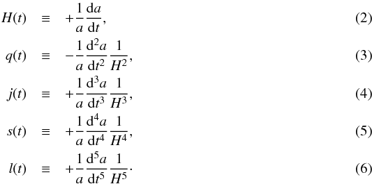 The cosmographic parameters, which are commonly indicated as the Hubble, deceleration, jerk, snap, and lerk parameters, correspond to the functions evaluated at the present time t0. Note that the use of the jerk parameter to distinguish between different models was also proposed in Sahni et al. (2003) and Alam et al. (2003) in the context of the statefinder parametrization. Furthermore, it is possible to relate the derivative of the Hubble parameter to the other cosmographic parameters
 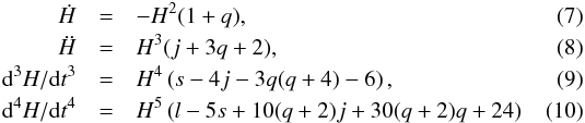 where a dot denotes derivative with respect to the cosmic time t. With these definitions the series expansion to the fifth order in time of the scale factor is
 ![Mathematical equation: \begin{eqnarray} \label{eq:a_series} \frac{a(t)}{a(t_{0})} &=& 1 + H_{0} (t-t_{0}) -\frac{q_{0}}{2} H_{0}^{2} (t-t_{0})^{2} +\frac{j_{0}}{3!} H_{0}^{3} (t-t_{0})^{3} \\ \nonumber &&+\frac{s_{0}}{4!} H_{0}^{4} (t-t_{0})^{4}+ \frac{l_{0}}{5!} H_{0}^{5} (t-t_{0})^{5} +\emph{O}[(t-t_{0})^{6}]. \end{eqnarray}](/articles/aa/full_html/2017/02/aa28911-16/aa28911-16-eq29.png) (11)From Eq. (11), and recalling that the distance traveled by a photon that is emitted at time t∗ and absorbed at the current epoch t0 is
(11)From Eq. (11), and recalling that the distance traveled by a photon that is emitted at time t∗ and absorbed at the current epoch t0 is 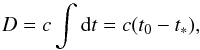 (12)we can construct the series for the luminosity or angular-diameter distance, whose expansions is
 (13)with
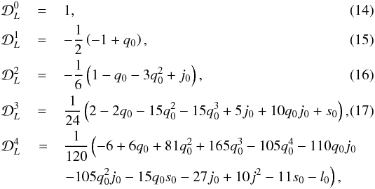 and
and  (18)with
 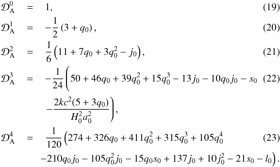 It is worth noting that since the cosmography is based on series expansions, the fundamental difficulties of applying this approach to fit the luminosity distance data using high-redshift distance indicators are connected with the convergence and truncation of the series. Recently, the possibility of attenuating the convergence problem has been analyzed by defining a new redshift variable, see Vitagliano et al. (2010), the so-called y-redshift,
  (24)For a series expansion in the classical z-redshift the convergence radius is equal to 1, which is a drawback when the application of cosmography is to be extended to redshifts z> 1. The y-redshift might help to solve this problem because the z-interval [0,∞] corresponds to the y-interval [0,1], so that we are mainly inside the convergence interval of the series, even for Cosmic Microwave Background data (z = 1089 → y = 0.999). In principle, we might therefore extend the series up to the redshift of decoupling, and place CMB-related constraints within the cosmographic approach. However, even using the series expansions in y-redshift, the problem of the series truncation remains (see also Zhan et al. 2016). The higher the order of the cosmographic expansion, the more accurate the approximation. However, as we add cosmographic parameters, the volume of the parameter space increases and the constraining strength could be weakened by degeneracy effects among different parameters. Therefore, the order of truncation depends on a compromise of different requirements. To fix a reliable expansion order of the cosmographic series, we first performed a qualitative analysis by fixing a fiducial model, given by the recently released Planck data Planck Collaboration XIII (2016), that is, a flat quintessence model, characterized by Ωm = 0.315 ± 0.017 and
  . The dimensionless Hubble function, E(z) associated with this model is
 (25)This model was used to construct a mock high-redshift Hubble diagram data set: we realized 500 simulations by randomly extracting the fiducial model parameters in their error range, and we also used the distribution of the most updated GRB Hubble diagram. For any redshift value we evaluated the mean and the dispersion of the distribution of the distance modulus, which characterize a normal probability function, from which the Hubble diagram data points are picked up. Finally, the exact values of the cosmographic parameters, derived from Eq. (25), were compared with the corresponding values of cosmographic series up to the fourth order, fitted on our mock data set. A significant degeneracy was detected in that even well-constrained cosmological parameters can correspond to larger uncertainties of the cosmographic parameters, which increase for higher order terms. This degeneracy can be only partially attributed to the accuracy of the cosmographic reconstruction: only q0 and j0 are well constrained. In the analysis we considered a forth-order expansion and were able to successfully set bounds on these parameters in a statistically consistent way.
It is worth to stress that the GRB Hubble diagram spans an optimal redshift range for the sensitivity of the observables quantities on the cosmological parameters, with special attention on the cosmography and its implications on dark energy. We show this in Fig. 1, following a simplified approach, in which we consider the distance modulus μ(z) as observable: we fixed a flat Λ cold dark matter (CDM) fiducial cosmological model by constructing the corresponding μfid(z,θ), and plot the percentage error on the distance modulus with respect to different corresponding functions randomly generated within an evolving CPL EOS. The higher sensitivity is only reached for  , that is, a redshift region unexplored by SNIa and BAO samples.
To provide reasonably narrow statistical constraints, we applied an MCMC method that allowed us to obtain marginalized likelihoods on the series coefficients, from which we infer tight constraints on these parameters. We have inserted several tests in our code that give us control over several physical requirements we expect from the theory. For instance, since we use data related to the Hubble parameter H(z), we are able to set restrictions on the Hubble parameter, H0 = H(0), and thus to obtain a considerable improvement in the quality of constraints.
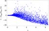 |
Fig. 1 z dependence of the percentage error in the distance modulus between the fiducial ΛCDM model and different flat models, with an evolving EOS |
3. Observational data sets
In our cosmographic approach we use the currently available observational data sets on SNIa and GRB Hubble diagram, and we set Gaussian priors on the distance data from the BAO and the Hubble constant h. These priors were included to help break the degeneracies of the parameters of the cosmographic series expansion in Eqs. (13).
3.1. Supernovae and GRB Hubble diagram
3.1.1. Supernovae Ia
In the past decade the confidence in type Ia supernovae as standard candles has steadily grown. SNIa observations gave the first strong indication of the recently accelerating expansion of the Universe. Since 1995, two teams of astronomers, the High-Z Supernova Search Team and the Supernova Cosmology Project, have been discovering type Ia supernovae at high redshifts. First results of the teams were published by Riess et al. (1998) and Perlmutter et al. (1999). Here we consider the recently updated Supernovae Cosmology Project Union 2.1 compilation Suzuki et al. (2012), which is an update of the original Union compilation and contains 580 SNIa, spanning the redshift range (0.015 ≤ z ≤ 1.4). We compare the theoretically predicted distance modulus μ(z) with the observed one through a Bayesian approach, based on the definition of the cosmographic distance modulus,  (26)where DL(zj, { θi }) is the Hubble free luminosity distance, expressed as a series depending on the cosmographic parameters, θi = (q0,j0,s0,l0). The parameter μ0 encodes the Hubble constant and the absolute magnitude M, and has to be marginalized over. Given the heterogeneous origin of the Union data set, we worked with an alternative version of the χ2:
  (27)where
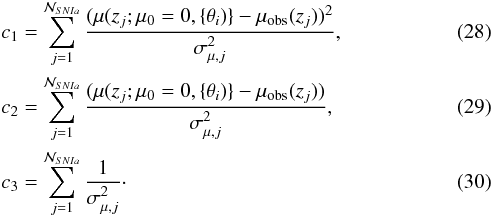 It is worth noting that
  (31)which clearly becomes minimum for μ0 = c2/c3, so that
  .
.
3.1.2. Gamma-ray burst Hubble diagram
Gamma-ray bursts are visible up to high redshifts thanks to the enormous energy that they release, and thus may be good candidates for our high-redshift cosmological investigation. However, GRBs may be everything but standard candles since their peak luminosity spans a wide range, even if there have been many efforts to make them distance indicators using some empirical correlations of distance-dependent quantities and rest-frame observables Amati et al. (2008). These empirical relations allow us to deduce the GRB rest-frame luminosity or energy from an observer-frame measured quantity, so that the distance modulus can be obtained with an error that depends essentially on the intrinsic scatter of the adopted correlation. We performed our cosmographic analysis using a GRB Hubble diagram data set, built by calibrating the Ep,i – Eiso relation. We recall that Eiso cannot be measured directly, but can be obtained through the knowledge of the bolometric fluence, denoted by Sbolo. This is more correctly  . Therefore Eiso depends on the GRB observable, Sbolo, but also on the cosmological parameters. At first glance, it seems that the calibration of these empirical laws depends on the assumed cosmological model. To use GRBs as tools for cosmology, this circularity problem has to be overcome, see for instance, Tsutsui et al. (2009), Li et al. (2008), Wang (2008), Wei (2010), Gao et al. (2012), Liang et al. (2008), Samushia & Ratra (2010), Liu & Wei (2015), Demianski & Piedipalumbo (2011), Demianski et al. (2011), Wang et al. (2015, 2016). In Paper I we have applied a local regression technique to estimate in a model-independent way the distance modulus from the Union SNIa sample.
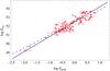 |
Fig. 2 Best-fit curves for the Ep,i – Eiso correlation relation superimposed on the data. The solid and dashed lines refer to the results obtained with the maximum likelihood (Reichart likelihood) and weighted χ2 estimator, respectively. |
When the correlation is fit (see Fig. 2) and its parameters are estimated, it is possible to compute the luminosity distance of a certain GRB at redshift z and, therefore, estimate the distance modulus for each ith GRB in our sample at redshift zi, and to build the Hubble diagram plotted in Fig. 3.
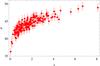 |
Fig. 3 Distance modulus μ(z) for the calibrated GRB Hubble diagram obtained by fitting the Ep,i – Eiso relation. |
3.2. Baryon acoustic oscillations data
Baryon acoustic oscillations data are promising standard rulers to investigate different cosmological scenarios and models. They are related to density fluctuations induced by acoustic waves that are created by primordial perturbations: the peaks of the acoustic waves gave rise to denser regions in the distribution of baryons, which, at recombination, imprint the correlation between matter densities at the scale of the sound horizon. Measurements of CMB radiation provide the absolute physical scale for these baryonic peaks, but the observed position of the peaks of the two-point correlation function of the matter distribution, compared with such absolute values, enables measuring cosmological distance scales. To use BAOs as a cosmological tool, we follow Percival et al. (2010) and define  (32)where zd is the drag redshift computed with the approximated formula in Eisenstein & Hu (1998), rs(z) is the comoving sound horizon,
  (33)and dV(z) the volume distance, that is,
 ![Mathematical equation: \begin{equation} d_V(z) = \left[\left(1+z\right) d_{\rm A}(z)^2\frac{c z}{H(z)}\right]^{\frac{1}{3}}\cdot\label{volumed} \end{equation}](/articles/aa/full_html/2017/02/aa28911-16/aa28911-16-eq84.png) (34)Here dA(z) is the angular diameter distance. Moreover, BAO measurements in spectroscopic surveys allow directly estimating the expansion rate H(z), converted into the quantity
(34)Here dA(z) is the angular diameter distance. Moreover, BAO measurements in spectroscopic surveys allow directly estimating the expansion rate H(z), converted into the quantity  , and constraints (from transverse clustering) on the comoving angular diameter distance DM(z), which in a flat FLRW metric is
  . To perform our analysis using BAO data, all these distances were properly developed in terms of the corresponding cosmographic series. The BAO data used in our analysis are summarized in Table 1 and are taken from Aubourg et al. (2015).
BAO data used in our analysis.
Here, the BAO scale rd is the radius of the sound horizon at the decoupling era, which can be approximated as ![Mathematical equation: \begin{equation} r_{\rm d} \approx {56.067\, \exp\left[-49.7 (\omega_\nu+0.002)^2\right] \over \omega_{cb}^{0.2436} \, \omega_b^{0.128876} \, [1+(\neff-3.046)/30.60] } ~{\rm Mpc}, \label{eqn:rdneff} \end{equation}](/articles/aa/full_html/2017/02/aa28911-16/aa28911-16-eq104.png) (35)for a standard radiation background with Neff = 3.046, ∑ mν< 0.6 eVων = 0.0107 ∑ mν/ 1.0 eV, see Aubourg et al. (2015). Using the values of ωb and ωcb derived by Planck, we find that rd = 147.49 ± 0.59 Mpc. It is worth noting that ωcb indicates the ω density of the baryons + CDM.
(35)for a standard radiation background with Neff = 3.046, ∑ mν< 0.6 eVων = 0.0107 ∑ mν/ 1.0 eV, see Aubourg et al. (2015). Using the values of ωb and ωcb derived by Planck, we find that rd = 147.49 ± 0.59 Mpc. It is worth noting that ωcb indicates the ω density of the baryons + CDM.
3.3. H(z) measurements
The measurements of Hubble parameters are a complementary probe to constrain the cosmological parameters and investigate the dark energy (Farroq et al. 2013; Farroq & Ratra 2013). The Hubble parameter, defined as  , where a is the scale factor, depends on the differential age of the Universe as a function of redshift and can be measured using the so-called cosmic chronometers. dz is obtained from spectroscopic surveys with high accuracy, and the differential evolution of the age of the Universe dt in the redshift interval dz can be measured provided that optimal probes of the aging of the Universe, that is, the cosmic chronometers, are identified Moresco et al. (2016). The most reliable cosmic chronometers at present are old early-type galaxies that evolve passively on a timescale much longer than their age difference, which formed the vast majority of their stars rapidly and early and have not experienced subsequent major episodes of star formation. Moreover, the Hubble parameter can also be obtained from the BAO measurements: by observing the typical acoustic scale in the light-of-sight direction, it is possible to extract the expansion rate of the Universe at a certain redshift Busca et al. (2013). We used a list of 28H(z) measurements, compiled in Farroq & Ratra (2013) and shown in Table 2.
Hubble parameter versus redshift data, as compiled in Farroq & Ratra (2013).
To also achieve a high accuracy approximation in terms of the proper cosmographic series for the H(z), we decided to consider only data with z< 0.9. We found that H(z) is much more sensitive to the order of the approximation and to the values of the cosmographic parameters than any distance observables. The relative error on H(z), δH, remains on the order of few percents only in this redshift range, as we show in Fig. 4.
4. Statistical analysis
To constrain the cosmographic parameters, we performed a preliminary and standard fitting procedure to maximize the likelihood function ℒ(p). This requires the knowledge of the precision matrix, that is, the inverse of the covariance matrix of the measurements, ![Mathematical equation: \begin{eqnarray} \footnotesize {\cal{L}}(\vec{p}) & \propto & \frac {\exp{(-\chi^2_{\rm SNIa/GRB}/2)}}{(2 \pi)^{\frac{{\cal{N}}_{\rm SNIa/GRB}}{2}} |\vec{C}_{\rm SNIa/GRB}|^{1/2}} \frac{\exp{(-\chi^2_{\rm BAO}/2})}{(2 \pi)^{{\cal{N}}_{\rm BAO}/2} |\vec{C}_{\rm BAO}|^{1/2}} \nonumber\\ & \times &~ \frac{1}{\sqrt{2 \pi \sigma_{\omega_{\rm m}}^2}} \exp{\left [- \frac{1}{2} \left ( \frac{\omega_{\rm m} - \omega^{\rm obs}_{\rm m}}{\sigma_{\omega_{\rm m}}} \right )^2\right]} ,\\ &&\times\frac{1}{\sqrt{2 \pi \sigma_h^2}} \exp{\left[- \frac{1}{2} \left ( \frac{h - h_{\rm obs}}{\sigma_h} \right )^2\right]} \frac{\exp{(-\chi^2_{\rm H}/2})}{(2 \pi)^{{\cal{N}}_{\rm H}/2} |\vec{C}_{\rm H}|^{1/2}}\nonumber \\ & \times & \frac{1}{\sqrt{2 \pi \sigma_{{\cal{R}}}^2}} \exp{\left [ - \frac{1}{2} \left ( \frac{{\cal{R}} - {\cal{R}}_{\rm obs}}{\sigma_{{\cal{R}}}} \right )^2 \right]} \nonumber \, \label{defchiall} \end{eqnarray}](/articles/aa/full_html/2017/02/aa28911-16/aa28911-16-eq119.png) (36)where
(36)where  (37)Here p is the set of parameters, N is the number of data points,
  is the ith measurement;
  indicate the theoretical predictions for these measurements and depend on the parameters p; Cij is the covariance matrix (specifically, CSNIa/GRB/H indicates the SNIa/GRBs/H covariance matrix); (hobs,σh) = (0.742,0.036) Riess et al. (2009), and
  Planck Collaboration XIII (2016). It is worth noting that the effect of our prior on h is not critical at all so that we are certain that our results are not biased by this choice. There are two opinions on h, one that claims it is centered on h = 0.68, and the other on h = 0.74 Chen & Ratra (2011), Sievers et al. (2013), Hinshaw et al. (2013), (Aubourg et al. 2015), and Planck Collaboration XIII (2016). In any event, we recall that the strongest dependence of the constraints on the assumed value of H0 is for the H(z) data alone. The term
 ![Mathematical equation: \hbox{$\displaystyle \frac{1}{\sqrt{2 \pi \sigma_{{\cal{R}}}^2}} \exp{\left [- \frac{1}{2} \left ( \frac{{\cal{R}} - {\cal{R}}_{\rm obs}}{\sigma_{{\cal{R}}}} \right )^2 \right]} $}](/articles/aa/full_html/2017/02/aa28911-16/aa28911-16-eq132.png) in the likelihood (37) considers the shift parameter ℛ:
in the likelihood (37) considers the shift parameter ℛ:  (38)where z⋆ = 1090.10 is the redshift of the surface of last scattering (Bond et al. 1997; Efstathiou & Bond 1999). According to the Planck data (ℛobs,σℛ) = (1.7407,0.0094).
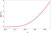 |
Fig. 4 Relative error between the exact Hubble parameter H(z) in the standard flat ΛCDM model (Ωm = 0.3, h = 0.7) and the corresponding cosmographic approximation: we need to limit our data set at z ≤ 0.9 when we wish to maintain an accuracy of a few percent. |
Finally, the term  in Eq. (37) takes into account some recent measurements of H(z) from the differential age of passively evolving elliptical galaxies. We used the data collected by (Stern et al. 2010) giving the values of the Hubble parameter for
  different points over the redshift range 0.10 ≤ z ≤ 1.75 with a diagonal covariance matrix. We finally performed our cosmographic analysis by considering a whole data set containing all the data sets, which we call the cosmographic data set. To sample the
  dimensional space of parameters, we used the MCMC method and ran five parallel chains and used the Gelman–Rubin diagnostic approach to test the convergence. As a test probe, it uses the reduction factor R, which is the square root of the ratio of the variance between-chain and the variance within-chain. A large R indicates that the between-chain variance is substantially greater than the within-chain variance, so that a longer simulation is needed. We require that R converges to 1 for each parameter. We set R−1 of order 0.05, which is more restrictive than the often used and recommended value R−1 < 0.1 for standard cosmological investigations. Moreover, to reduce the uncertainties of the cosmographic parameters, since methods like the MCMC are based on an algorithm that moves randomly in the parameter space, we a priori impose in the code some basic consistency controls requiring that all of the (numerically) evaluated values of H(z) and dL(z) be positive. As first step, we performed a sort of pre-statistical analysis to select the starting points of the full analysis: we ran our chains to compute the likelihood in Eq. (37) considering only the SNIa. Therefore we applied the same MCMC approach to evaluate the likelihood in Eq. (37), combining the SNIa, H(z), and the BAO data with the GRBs Hubble diagram, as described above. We discarded the first 30% of the point iterations at the beginning of any MCMC run, and thinned the chains that were run many times. We finally extracted the constraints on cosmographic parameters by coadding the thinned chains. The histograms of the parameters from the merged chains were then used to infer median values and confidence ranges: the 15.87th and 84.13th quantiles define the 68% confidence interval; the 2.28th and 97.72th quantiles define the 95% confidence interval; and the 0.13th and 99.87th quantiles define the 99% confidence interval. In Tables 3–5 we present the results of our analysis. Only the deceleration parameter, q0, and the jerk, j0, are well constrained (see also Fig. 5); the snap parameter, s0, is weakly constrained, and the lerk, l0, is unconstrained, as has been found in the literature (see Demianski et al. 2012; Lazkoz et al. 2010).
Constraints on the cosmographic parameters from combining the SNIa Hubble diagram with the BAO and H(z) data sets (Cosmography Ia).
Constraints on the cosmographic parameters from combining the GRBs Hubble diagram with the BAO and H(z) data sets (Cosmography Ib).
Constraints on the cosmographic parameters from combining the SNIa and GRBs Hubble diagrams with the BAO data set (Cosmography II).
Our statistical MCMC analysis shows that the deceleration parameter q0 is clearly negative in all the cases. The marginal likelihood distributions for the current values of the deceleration parameter q0 and the jerk j0 indicate an only negligible probability for q0> 0, and that j0 is significantly different from its ΛCDM value j0 = 1. In Fig. 5 we show the confidence regions for q0, and j0: the left and the right panels show the results obtained by using only the GRBs data set (Cosmography Ib) or the whole sample (Cosmography II); the GRB data mainly constrain the jerk parameter.
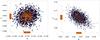 |
Fig. 5 Confidence regions in the (q0−j0) plane, as provided by Cosmography Ib and II. The inner brown region defines the 2σ confidence level. The parameters q0 and j0 are well constrained, the values q0> 0 are ruled out, the value j0 = 1 (which is the ΛCDM value) is statistically not favorable. On the axes we also plot the box-and-whisker diagrams for the respective parameters: the bottom and top of the diagrams are the 25th and 75th percentile (the lower and upper quartiles, respectively), and the band near the middle of the box is the median. |
5. Connection with the dark energy EOS
As already mentioned, within the FLRW paradigm, all possibilities of interpreting the dark energy can be characterized, as far as the background dynamics is concerned, by an effective dark energy EOS w(z). Extracting information on the EOS of dark energy from observational data is therefore both an issue of crucial importance and a challenging task. To probe the dynamical evolution of dark energy, we can parameterize w(z) empirically by assuming that it evolves smoothly with redshift and can be approximated by some analytical expression, containing two or more free parameters. Since any analytical form of w(z) is not based on a grounded theory, in principle an extreme flexibility is required, which means a large numbers of parameters. However, at present, the precision in the observational data is not good enough to provide constraints for more than a few parameters (two or three at most). Often, to reduce the huge arbitrariness, the space of allowed w(z) models is restricted to consider only w(z) ≥ −1. If w(z) is an effective EOS parameterizing a modified gravity theory, for instance, a scalar-tensor or an f(R) model, then this constraint might be too restrictive and partially arbitrary. Whereas we account the cosmography results as a sort of constraint on the EOS space parameters. It is well known that the connection between the cosmographic and the dark energy parametrization is based on the series expansion of the Hubble function H(z). For a spatially flat cosmological model we have  where
where  , and w(z) parameterizes the dark energy EOS. We have
 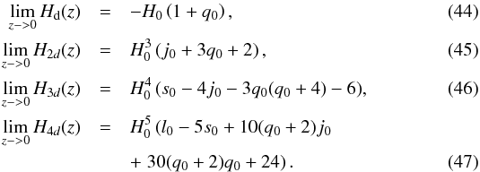 It is worth noting that the possibility of inverting Eqs. ((44)–(47)) strongly depends on the number of cosmographic parameters we are working with and on how many parameters enter the dark energy EOS. For instance, if we expect that only two cosmographic parameters, (q0,j0), are well constrained, it is possible to derive information about a constant dark energy model and estimate Ωm as
 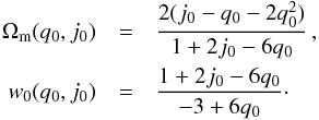 (48)If Ωm is considered as a free parameter, then with the same cosmographic parameters, (q0,j0), we can also derive some information about a dynamical dark energy model. In our investigation we preferred this conservative approach. All the statistical properties of the dark energy parameters (median, error bars, etc.) can be directly extracted from the cosmographic samples we have obtained from the MCMC analysis. However, it is worth noting that since the map described by Eqs. ((44)–(47)) is non-linear, the equations admit multiple solutions for any assigned n-fold (q0, j0, s0,...): to improve the maximum likelihood estimate, we incorporated the restrictions on the EOS parameters coming from cosmography by constructing a sort of constrained optimizer within the MCMCs. In this analysis we considered the CPL model (Chevallier & Polarski 2001; Linder 2003), where
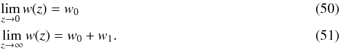
 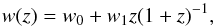 (49)where w0 and w1 are free, fitting parameters, characterized by the property that
This parametrization describes a wide variety of scalar field dark energy models and therefore achieves a good compromise to construct a model independent analysis. The results of the cosmographic analysis allow us to infer the values of w0 and w1, thus providing constraints on the dynamical nature of the dark energy. The EOS is evolving, as illustrated, for example, in Fig. 6 compared to the CPL model, thus reflecting, at 1σ, the possibility of a deviation from the ΛCDM cosmological model, as has been indicated by previous investigations (see, for instance, Paper 1)
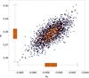 |
Fig. 6 Confidence regions in the (w0−w1) plane, as provided by Cosmography II, for the CPL parametrization of the dark energy. The inner brown region defines the 2σ confidence level. These parameters are well constrained, and the values w0 = −1, and w1 = −1 (which characterize the standard ΛCDM model) are statistically not favorable. The bottom and top of the diagrams plotted on the axes correspond to the 25th and 75th percentile, and the band near the middle of the box is the median. |
5.1. Precision cosmography from generalized Padé approximation: stronger constraints for the dark energy parametrization
Padé approximation generalizes the Taylor series expansion of a function f(z): it is well known that if the series converges absolutely to an infinitely differentiable function, then the series defines the function uniquely and the function uniquely defines the series. The Padé approach provides an approximation for f(z) through rational functions. As an illustrative example we consider a given power series  (52)where
  where m ≤ n. The rational function
  is a Padé approximation to the series f(z) and
  (55)that is, the lowest order monom in the difference
 is on the order of m + n + 1. Equation (55) imposes some requirements on R and its derivatives:
where k = 1,...m + n. Equations ((55), (57)) provide m + n + 2 equations for the unknowns a0,...am, b0,...bn. Since this system is, obviously, undetermined, the normalization b0 = 1 is generally used. A long-standing interest in rational fractions and related topics (such as the Padé approximation) is observed in pure mathematics, numerical analysis, physics, and chemistry. There is a growing interest today in applying the Padé approximation technique to the accelerated Universe cosmology to investigate the nature of dark energy (Nesseris & Garcia-Bellido 2013; Gruber & Luongo 2014; Aviles et al. 2014; and Liu & Wei 2015). To construct an accurate generalized Padé approximation of the distance modulus and investigate the implications on the cosmography, we here started from a two-parameter a,b Padé approximation for the deceleration parameter q(z), and obtained H(z) and the luminosity distance dL(z) according to the relations, here we assume a flat cosmological model,  For H(z) we obtain a power-law approximation with fixed exponent, and for dL an exact analytical expression in terms of the Gauss hypergeometric function,
  :
:
![Mathematical equation: \begin{eqnarray} && d_L(z)=\frac{c}{100 h} \frac{(z+1) (\beta +1)^{\frac{\alpha +\beta \gamma }{\beta \delta }}}{\gamma }\\ &&\qquad\qquad\times \left[(z+1)^{\gamma } \, _2F_1\left(\frac{\gamma }{\delta },\frac{\alpha +\beta \gamma }{\beta \delta };\frac{\gamma }{\delta }+1;-(z+1)^{\delta } \beta \right)\right.\nonumber\\ &&\left.\qquad \qquad- _2F_1\left(\frac{\gamma }{\delta },\frac{\alpha +\beta \gamma }{\beta \delta };\frac{\gamma }{\delta }+1;-\beta \right)\right]\nonumber, \label{dlpade} \end{eqnarray}](/articles/aa/full_html/2017/02/aa28911-16/aa28911-16-eq230.png) (60)where α, β, γ and δ are fitting parameters. This extendedPadé approximation works even better than the original approximation, as shown in Fig. (7), where we evaluate the relative error between a randomly generated high-redshift ΛCDM Hubble diagram and its extended Padé approximation. The parameters α, β, γ, and δ have been constrained using the same statistical analysis described previously, that is, by implementing the MCMC simulations and simultaneously computing the full probability density functions of these parameters. It is, moreover, possible to map the extended Padé parameters into the cosmographic parameters, allowing a refined statistics of its specific parameters (especially q0 and j0) and, at last, stronger constraints on the dark energy EOS. The values q0> 0 are significantly ruled out, and the indications favoring the value j0 ≠ 1 are much stronger than in the cosmographic analysis. Equations ((44)–(47)) allow projecting the constraints obtained from the Padé analysis on the space of the EOS parameters: a dynamical dark energy is strongly supported by this analysis, as shown in Table 6, compared to the CPL parametrization.
(60)where α, β, γ and δ are fitting parameters. This extendedPadé approximation works even better than the original approximation, as shown in Fig. (7), where we evaluate the relative error between a randomly generated high-redshift ΛCDM Hubble diagram and its extended Padé approximation. The parameters α, β, γ, and δ have been constrained using the same statistical analysis described previously, that is, by implementing the MCMC simulations and simultaneously computing the full probability density functions of these parameters. It is, moreover, possible to map the extended Padé parameters into the cosmographic parameters, allowing a refined statistics of its specific parameters (especially q0 and j0) and, at last, stronger constraints on the dark energy EOS. The values q0> 0 are significantly ruled out, and the indications favoring the value j0 ≠ 1 are much stronger than in the cosmographic analysis. Equations ((44)–(47)) allow projecting the constraints obtained from the Padé analysis on the space of the EOS parameters: a dynamical dark energy is strongly supported by this analysis, as shown in Table 6, compared to the CPL parametrization.
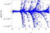 |
Fig. 7 Percentage error between a randomly generated high-redshift ΛCDM Hubble diagram and its generalized Padé approximation: this approximation is more accurate. |
Median (best fit), mean values, and confidence regions in the (w0-w1) plane, by projecting the constraints from the generalized Padé approximation on the space of the EOS parameters.
6. Conclusions
We investigated the dynamics of the Universe by using a cosmographic approach: we performed a high-redshift analysis that allowed us to set constraints on the cosmographic expansion up to the fifth order, based on the Union2 SNIa data set, the GRB Hubble diagram, constructed by calibrating the correlation between the peak photon energy, Ep,i, and the isotropic equivalent radiated energy, Eiso, and Gaussian priors on the distance from the BAO, and the Hubble constant h (these priors were included to help break the degeneracies among model parameters). Our statistical analysis was based on MCMC simulations to simultaneously compute the regions of confidence of all the parameters of interest. Since methods like the MCMC are based on an algorithm that randomly probes the parameter space, to improve the convergence, we imposed some constraints on the series expansions of H(z) and dL(z), requiring that in each step of our calculations dL(z) > 0, and H(z) > 0. We performed the same MCMC calculations, first considering the SNIa Hubble diagram and the BAO data sets or the GRBs Hubble diagram, and the BAO data sets separately (Cosmography Ia and Ib, respectively), and then constructing an overall data set joining them together (Cosmography II). Our MCMC method allowed us to obtain constraints on the parameter estimation, in particular for higher order cosmographic parameters (the jerk and the snap). The deceleration parameter confirms the current acceleration phase; the estimation of the jerk reflects at 1σ the possibility of a deviation from the ΛCDM cosmological model. Moreover, we investigated implications of our results for the reconstruction of the dark energy EOS by comparing the standard technique of cosmography with an alternative approach based on generalized Padé approximations of the same observables. Owing to the better convergence properties of these expansions, it is possible to improve the constraints on the cosmographic parameters and also on the dark matter EOS: our analysis indicates that at the 1σ level the dark energy EOS is evolving.
Acknowledgments
M.D. is grateful to the INFN for financial support through the Fondi FAI GrIV. E.P. acknowledges the support of INFN Sez. di Napoli (Iniziative Specifica QGSKY and TEONGRAV). L.A. acknowledges support by the Italian Ministry for Education, University and Research through PRIN MIUR 2009 project on Gamma ray bursts: from progenitors to the physics of the prompt emission process (ERC3HT Prot. 2009).
References
- Akarsu, Ö, Bouhmadi-López, M., Brilenkov, M., et al. 2015, JCAP, 7, 38 [NASA ADS] [CrossRef] [Google Scholar]
- Alam, U., Sahni, V., Saini, T. D., & Starobinsky, A. A. 2003, MNRAS, 344, 1057 [NASA ADS] [CrossRef] [Google Scholar]
- Amati, L., Guidorzi, C., Frontera, F., et al. 2008, MNRAS, 391, 577 [NASA ADS] [CrossRef] [MathSciNet] [Google Scholar]
- Aubourg., E., Bailey, S., Bautista, J. E., et al. (BOSS Collaboration) 2015, Phys. Rev. D, 92, 123516 [NASA ADS] [CrossRef] [Google Scholar]
- Aviles, A., Bravetti, A., Capozziello, S., & Luongo, O. 2014, Phys. Rev. D, 90, 043531 [NASA ADS] [CrossRef] [Google Scholar]
- Astier, P., Guy, J., Regnault, N., et al. 2006, A&A, 447, 31 [NASA ADS] [CrossRef] [EDP Sciences] [Google Scholar]
- Bond, J. R., Efstathiou, G., & Tegmark, M. 1997, MNRAS, 291, L33 [NASA ADS] [Google Scholar]
- Busca, N. G., Delubac, T., Rich, J., et al. 2013, A&A, 552, A96 [NASA ADS] [CrossRef] [EDP Sciences] [Google Scholar]
- Capozziello, S., Lazkoz, R., & Salzano, V. 2011, Phys. Rev. D, 84, 124061 [NASA ADS] [CrossRef] [Google Scholar]
- Chen, G., & Ratra, B. 2011, PASP, 123, 1127 [NASA ADS] [CrossRef] [Google Scholar]
- Chevallier, M., & Polarski, D. 2001, Int. J. Mod. Phys. D, 10, 213 [NASA ADS] [CrossRef] [Google Scholar]
- Demianski, M., & Piedipalumbo, E. 2011, MNRAS, 415, 3580 [NASA ADS] [CrossRef] [Google Scholar]
- Demianski, M., Piedipalumbo, E., & Rubano, C. 2011, MNRAS, 411, 1213 [NASA ADS] [CrossRef] [Google Scholar]
- Demianski, M., Piedipalumbo, E., Rubano, C., & Scudellaro, P. 2012, MNRAS, 426, 1396 [NASA ADS] [CrossRef] [Google Scholar]
- Demianski, M., Piedipalumbo, E., Sawant, D., & Amati, L. 2017, A&A, 598, A112 (Paper I) [NASA ADS] [CrossRef] [EDP Sciences] [Google Scholar]
- Eisenstein, D. J., & Hu, W. 1998, ApJ, 496, 605 [NASA ADS] [CrossRef] [Google Scholar]
- Efstathiou, G., & Bond, J. R. 1999, MNRAS, 304, 75 [NASA ADS] [CrossRef] [MathSciNet] [Google Scholar]
- Farroq, O., & Ratra, B. 2013, ApJ, 766, L7 [NASA ADS] [CrossRef] [MathSciNet] [Google Scholar]
- Farroq, O., Mania, D., & Ratra, B. 2013, ApJ, 764, 13 [CrossRef] [Google Scholar]
- Gao, H., Liang, N., & Zhu, Z.-H. 2012, Int. J. Mod. Phys. D, 21, 1250016 [NASA ADS] [CrossRef] [Google Scholar]
- Gruber, C., & Luongo, O. 2014, Phys. Rev. D, 89, 103506 [NASA ADS] [CrossRef] [Google Scholar]
- Hinshaw, G., Larson, D., Komatsu, E., Spergel, D. N., & Bennett, C. L. 2013, ApJS, 19, 208 [Google Scholar]
- Lazkoz, R., Lazkoz, A. J., Escamilla-Rivera, C., Salzano, V., & Sendra, I. 2010, JCAP, 12, 5 [NASA ADS] [Google Scholar]
- Li, H., Su, M., Fan, Z., Dai, Z., & Zhang, X. 2008, Phys. Lett. B, 658, 95 [Google Scholar]
- Liang, N., Xiao, W. K., Liu, Y., & Zhang, S. N. 2008, ApJ, 685, 354 [NASA ADS] [CrossRef] [Google Scholar]
- Liu, J., & Wei, H. 2015, Gen. Rel. Grav., 47, 141 [NASA ADS] [CrossRef] [Google Scholar]
- Linder, E. V. 2003, Phys. Rev. Lett., 90, 091301 [NASA ADS] [CrossRef] [PubMed] [Google Scholar]
- Moresco, M., Pozzetti, L., Cimatti, A., et al. 2016, JCAP, 05, 014 [NASA ADS] [CrossRef] [Google Scholar]
- Nesseris, S., & Garcia-Bellido, J. 2013, Phys. Rev. D, 88, 063521 [Google Scholar]
- Peebles, P. J. E., & Ratra, B. 1988, ApJ, 325, 17 [Google Scholar]
- Ratra, B., & Peebles, P. J. E. 1988, Phys. Rev. D, 37, 3406 [NASA ADS] [CrossRef] [MathSciNet] [Google Scholar]
- Planck Collaboration XVI. 2014, A&A, 571, A16 [NASA ADS] [CrossRef] [EDP Sciences] [Google Scholar]
- Planck Collaboration XIII. 2016, A&A, 594, A13 [NASA ADS] [CrossRef] [EDP Sciences] [Google Scholar]
- Percival, W. J., Reid, B. A., Eisenstein, D. J., et al. 2010, MNRAS, 401, 2148 [NASA ADS] [CrossRef] [Google Scholar]
- Perlmutter, S., Aldering, G., & Goldhaber, G., et al. 1999, ApJ, 517, 565 [NASA ADS] [CrossRef] [Google Scholar]
- Riess, A. G., Filippenko, A. V., Challis, P., et al. 1998, ApJ, 116, 1009 [Google Scholar]
- Riess, A. G., Strolger, L. G., Casertano, S., et al. 2007, ApJ, 659, 98 [NASA ADS] [CrossRef] [Google Scholar]
- Riess, A. G., Macri, L., Li, W., et al. 2009, ApJ, 699, 539 [NASA ADS] [CrossRef] [Google Scholar]
- Riess, A. G., Macri, L., Casertano, S., Lampeitl, H., & Ferguson, H. C. 2011, ApJ, 730, 119 [NASA ADS] [CrossRef] [Google Scholar]
- Sahni, V., Saini, T. D., Starobinsky, A. A., & Alam, U. 2003, JETP Lett., 77, 201 [Google Scholar]
- Samushia, L., & Ratra, B. 2010, ApJ, 714, 1347 [NASA ADS] [CrossRef] [Google Scholar]
- Sievers, J. L., Hlozek, R. A., Nolta, M. R., Acquaviva, V., & Addison, G. E. 2013, JCAP, 60, 1310 [Google Scholar]
- Suzuki, N., Rubin, D., Lidman, C., et al. (The Supernova Cosmology Project) 2012, ApJ, 746, 85 [NASA ADS] [CrossRef] [Google Scholar]
- Tsutsui, R., Nakamura, T., Yonetoku, D., et al. 2009, MNRAS, 394, L31 [NASA ADS] [CrossRef] [Google Scholar]
- Visser, M. 2004, Class. Quant. Grav., 21, 2603 [NASA ADS] [CrossRef] [Google Scholar]
- Vitagliano, V., Xia, J. Q., Liberati, S., & Viel, M. 2010, JCAP, 3, 005 [NASA ADS] [CrossRef] [Google Scholar]
- Wang, Y. 2008, Phys. Rev. D, 78, 123532 [NASA ADS] [CrossRef] [Google Scholar]
- Wang, J., Deng, J. S., & Qiu, Y. J. 2008, Chin. J. Astron. Astrophys., 8, 255 [NASA ADS] [CrossRef] [Google Scholar]
- Wang, F. Y., Dai, Z. G., & Liang, E. W. 2015, New Astron. Rev., 67, 1 [NASA ADS] [CrossRef] [Google Scholar]
- Wang, J. S., Wang, F. Y., Cheng, K. S., & Dai, Z. G. 2016, A&A, 585, A68 [NASA ADS] [CrossRef] [EDP Sciences] [Google Scholar]
- Wei, H. 2010, JCAP, 8, 20 [NASA ADS] [CrossRef] [Google Scholar]
- Zhang, M.-J., Li, H., & Xia, J.-Q. 2016, ArXiv e-prints [arXiv:1601.01758] [Google Scholar]
All Tables
Constraints on the cosmographic parameters from combining the SNIa Hubble diagram with the BAO and H(z) data sets (Cosmography Ia).
Constraints on the cosmographic parameters from combining the GRBs Hubble diagram with the BAO and H(z) data sets (Cosmography Ib).
Constraints on the cosmographic parameters from combining the SNIa and GRBs Hubble diagrams with the BAO data set (Cosmography II).
Median (best fit), mean values, and confidence regions in the (w0-w1) plane, by projecting the constraints from the generalized Padé approximation on the space of the EOS parameters.
All Figures
|
Fig. 1 z dependence of the percentage error in the distance modulus between the fiducial ΛCDM model and different flat models, with an evolving EOS |
| In the text | |
|
Fig. 2 Best-fit curves for the Ep,i – Eiso correlation relation superimposed on the data. The solid and dashed lines refer to the results obtained with the maximum likelihood (Reichart likelihood) and weighted χ2 estimator, respectively. |
| In the text | |
|
Fig. 3 Distance modulus μ(z) for the calibrated GRB Hubble diagram obtained by fitting the Ep,i – Eiso relation. |
| In the text | |
|
Fig. 4 Relative error between the exact Hubble parameter H(z) in the standard flat ΛCDM model (Ωm = 0.3, h = 0.7) and the corresponding cosmographic approximation: we need to limit our data set at z ≤ 0.9 when we wish to maintain an accuracy of a few percent. |
| In the text | |
|
Fig. 5 Confidence regions in the (q0−j0) plane, as provided by Cosmography Ib and II. The inner brown region defines the 2σ confidence level. The parameters q0 and j0 are well constrained, the values q0> 0 are ruled out, the value j0 = 1 (which is the ΛCDM value) is statistically not favorable. On the axes we also plot the box-and-whisker diagrams for the respective parameters: the bottom and top of the diagrams are the 25th and 75th percentile (the lower and upper quartiles, respectively), and the band near the middle of the box is the median. |
| In the text | |
|
Fig. 6 Confidence regions in the (w0−w1) plane, as provided by Cosmography II, for the CPL parametrization of the dark energy. The inner brown region defines the 2σ confidence level. These parameters are well constrained, and the values w0 = −1, and w1 = −1 (which characterize the standard ΛCDM model) are statistically not favorable. The bottom and top of the diagrams plotted on the axes correspond to the 25th and 75th percentile, and the band near the middle of the box is the median. |
| In the text | |
|
Fig. 7 Percentage error between a randomly generated high-redshift ΛCDM Hubble diagram and its generalized Padé approximation: this approximation is more accurate. |
| In the text | |
Current usage metrics show cumulative count of Article Views (full-text article views including HTML views, PDF and ePub downloads, according to the available data) and Abstracts Views on Vision4Press platform.
Data correspond to usage on the plateform after 2015. The current usage metrics is available 48-96 hours after online publication and is updated daily on week days.
Initial download of the metrics may take a while.