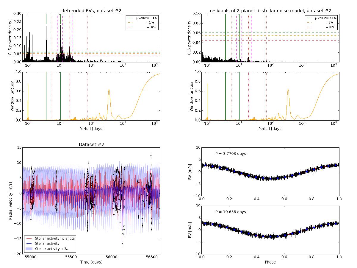
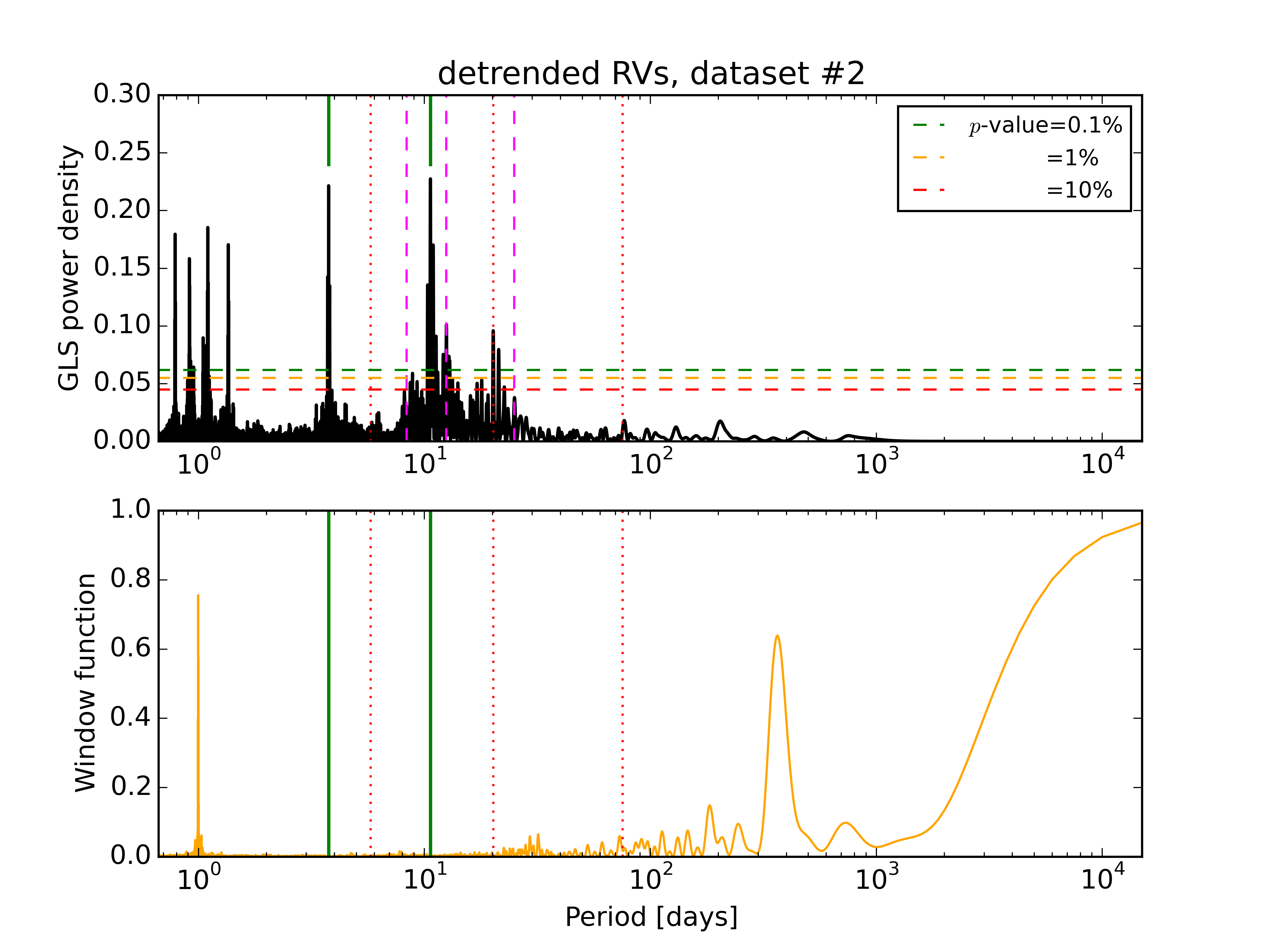
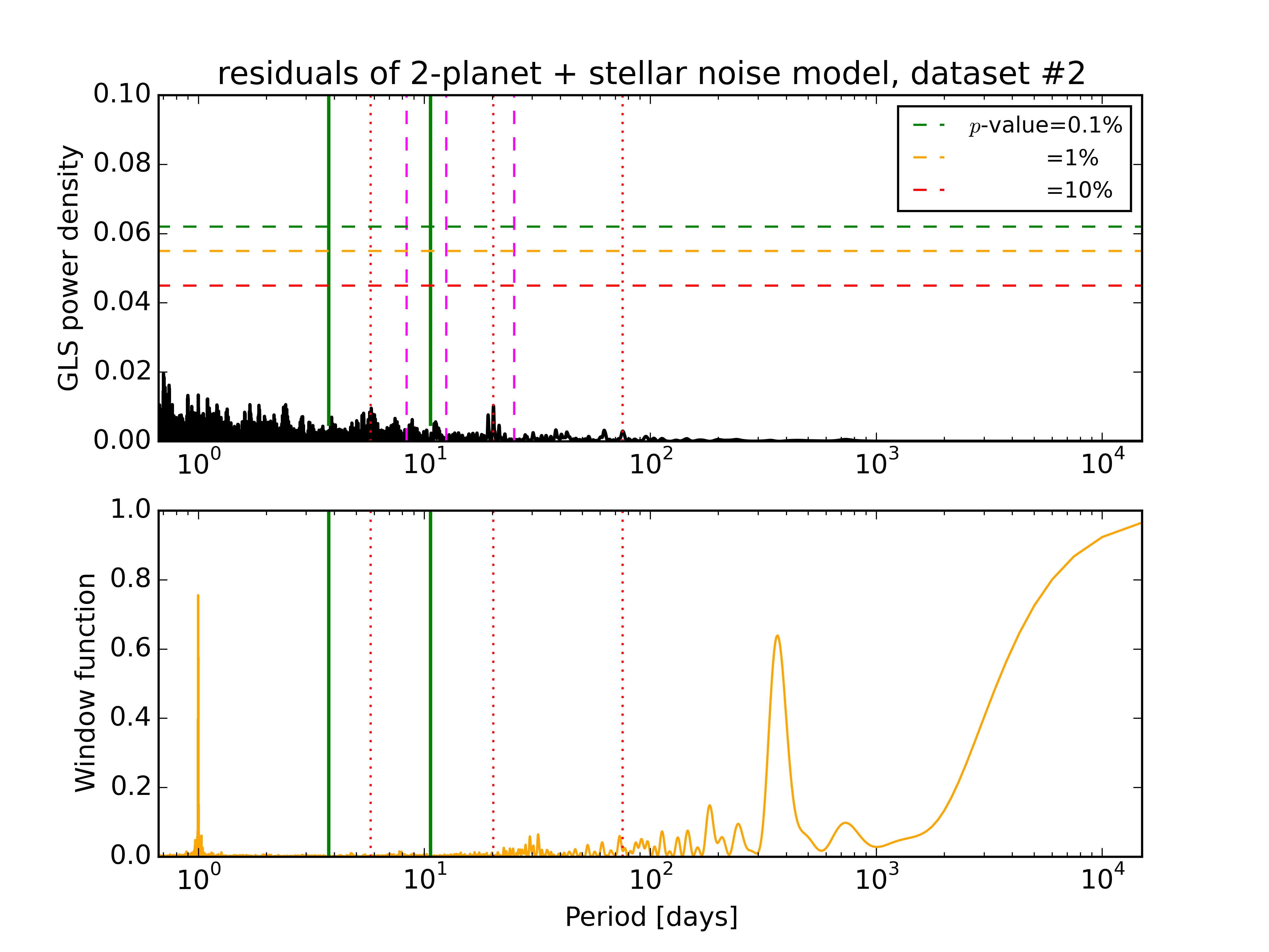
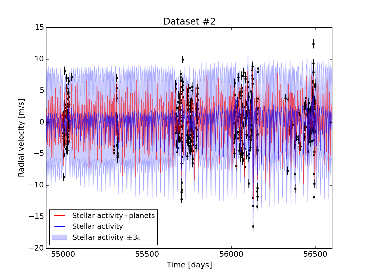
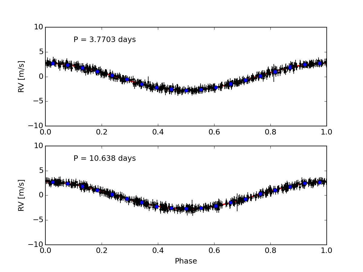
Top left panel: GLS periodogram of the challenge RV data set number 2 analysed by the team 1, and the corresponding window function. The original RVs data were first corrected through a linear regression with ) and then through a sinusoidal fit to remove a 2727-day periodicity likely related to a long-term stellar activity cycle. Vertical lines indicate i) the orbital frequencies of the planetary candidates identified by the team (solid green lines), which turned out to be real; ii) the missed planets (dotted red lines); iii) the simulated stellar rotation period and its first two harmonics (dashed magenta lines). Top right panel: GLS periodogram of the RV residuals after the best-fit global model including the two planets detected was removed from the detrended data set. A bootstrap analysis performed on these RV residuals shows no evidence of significant signals left. Bottom left panel: RVs detrended with the best-fit global model superposed (solid red line) and the mean contribution due to the stellar activity predicted by the GP (blue solid line). The shaded area spans the 3σ region centered around the best-fit noise model. Bottom right panel: RV curves folded at the periods of the two candidate Keplerian solutions found by the team, with the superposed red continuous line representing the best-fit orbital model. Data in each plot refers to a single planet, and are obtained from the original RVs by subtracting the offset, the GP stellar activity noise model, and the Keplerian of the other planet.