| Issue |
A&A
Volume 597, January 2017
|
|
|---|---|---|
| Article Number | A87 | |
| Number of page(s) | 11 | |
| Section | Stellar structure and evolution | |
| DOI | https://doi.org/10.1051/0004-6361/201629511 | |
| Published online | 06 January 2017 | |
Evolutionary history of four binary blue stragglers from the globular clusters ω Cen, M 55, 47 Tuc, and NGC 6752
1 Warsaw University Observatory, Al. Ujazdowskie 4, 00-478 Warsaw, Poland
e-mail: This email address is being protected from spambots. You need JavaScript enabled to view it.
2 Nicolaus Copernicus Astronomical Center, Bartycka 18, 00-716 Warsaw, Poland
e-mail: This email address is being protected from spambots. You need JavaScript enabled to view it.
; This email address is being protected from spambots. You need JavaScript enabled to view it.
Received: 10 August 2016
Accepted: 30 September 2016
Abstract
Context. Origin and evolution of blue stragglers in globular clusters is still a matter of debate.
Aims. The aim of the present investigation is to reproduce the evolutionary history of four binary blue stragglers in four different clusters, for which precise values of global parameters are known.
Methods. Using the model for cool close binary evolution that we developed, progenitors of all investigated binaries were found and their parameters evolved into the presently observed values.
Results. The results show that the progenitors of the binary blue stragglers are cool close binaries with period of a few days, which transform into stragglers by rejuvenation of the initially less massive component as a result of mass transfer from its more massive companion overflowing the inner critical Roche surface. The parameters of V209 from ω Cen indicate that the binary is substantially enriched in helium. This is an independent and strong evidence of the existence of the helium rich subpopulation in this cluster.
Key words: stars: evolution / binaries: close / globular clusters: general / blue stragglers
© ESO, 2017
1. Introduction
Blue stragglers (BS) are usually defined as objects brighter and bluer than the main-sequence turn-off point of their host cluster (Sandage 1953). In the color−magnitude diagram (CMD) they occupy an extension of the main sequence (MS), from which all normal stars at the age of the cluster would have evolved billions of years ago. In other words, they indeed seem to lag in time, or straggle, behind the bulk of the cluster (Shara et al. 1997). Their location in the CMD suggests typical masses of 1.0−1.5 M⊙− significantly larger than those of normal stars in globular clusters (GC). Because of this, BSs are thought to have increased their mass during their evolution. Two basic ideas have been proposed to explain the origin of these objects: direct stellar collisions (Hills & Day 1976), and mass transfer between or coalescence of the components of binary systems (McCrea 1964; Chen & Han 2008, and references therein) forming, respectively, collisional and evolutionary BSs. The role of each of these scenarios in producing the observed BS populations is still debated (Ferraro et al. 2012, and references therein; Chatterjee et al. 2013; Perets 2015). It is conceivable that different intracluster environments could be responsible for different origins of BSs: in less dense clusters they would preferentially form as evolutionary mergers of, or owing to mass transfer in close binaries while, in high-density ones, from collisions during dynamical encounters between binaries and/or single stars (Chatterjee et al. 2013; Hypki & Giersz 2013).
BSs are not rare objects: every GC has been observed as hosting them, and each GC can contain from a not many up to a few hundred of them. The resulting straggler fractions range from a few times 10-5 to 10-4 (Piotto et al. 2004), however their presence in a cluster is far from insignificant. They result from the fascinating interplay between stellar evolution and stellar dynamics which drives cluster evolution (Cannon 2015) and, as such, they represent a crucial link between standard stellar evolution and internal dynamics of GCs (Ferraro et al. 2015). Thus, by studying them, the dynamical history of a cluster can be constructed, and important constraints obtained on the role played by cluster dynamics on the evolution of cluster members. BS statistics can also provide constraints on the initial distribution of binary systems (Hypki & Giersz 2013). All these factors explain why, within the last twenty years, BSs have evolved from a marginal oddity into an attractive subject of interest for at least three astronomical specialties: observers, cluster evolution modelers, and stellar/binary evolution modelers.
Observational data on which our paper is based have been collected within the Cluster AgeS Experiment (CASE) project. The main aim of CASE is to determine the basic stellar parameters (masses, luminosities, and radii) of the components of GC binaries to a precision better than 1% to measure ages and distances of their parent clusters, and to test stellar evolution models (Kaluzny et al. 2005). The best-suited objects for this type of survey are well-detached binaries so evolutionarily advanced that at least one component is about to leave (or has just left) the main sequence. A by-product of the systematic search for such systems is a wealth of cluster variables. Among the latter about 20 binary BSs have been found (Kaluzny et al. 2013a,b, 2014, 2015a, 2016) which strongly supports the mass transfer option. The aim of the present paper is to verify if a consistent evolutionary scenario can be obtained for these type of objects based on the available data.
To the best of our knowledge, the four stragglers whose evolutionary history we attempt to reconstruct are the only ones in GCs whose parameters are accurately (or at least reasonably accurately) known. In Sect. 2 we discuss their properties together with observational limits on their chemical composition and age. Section 3 briefly introduces the evolutionary code employed to follow their evolution. Section 4 presents results of the search for their progenitors. The results are discussed in Sect. 5, and the paper is summarized in Sect. 6.
2. Observational data
The subject of the present investigation is binary blue stragglers V209/ω Cen, V60/M 55, V228/47 Tuc, and V8/NGC 6752 (hereafter: V209, V60, V228 and V8, respectively). The parameters of all the four systems (orbital period P, semi-major axis of the orbit a, component masses M1 and M2, component radii R1 and R2, effective temperatures of the components T1 and T2) are collected in Table 1, together with ages and chemical compositions or their parent clusters. We note that the quoted temperature uncertainties include the spread of color-temperature calibrations used but, accounting for discrepancies among the various calibrations, they might be increased to 250−300 K for V60 (a synthetic calibration was employed; see Rozyczka et al. 2013, for a justification) and V228 (T1 was found iteratively, and its error was difficult to estimate, see Kaluzny et al. 2007b).
2.1. Binaries
2.1.1. V209
V209 was discovered by Kaluzny et al. (1996) during a search for variable stars in the field of ω Centauri. The light curve exhibits total eclipses and is nearly flat between the minima, indicating a detached system. A detailed account from photometric and spectroscopic observations can be found in Kaluzny et al. (2007a), who also derive absolute parameters of the components. On the CMD of the cluster (their Fig. 8), the primary component is located at the tip of the BS region, while the much fainter (ΔV ≈ 1.5 mag) secondary approaches the hot subdwarf (sdB) domain.
Parameters derived from observations.
In the evolutionary scenario proposed by Kaluzny et al. (2007a), V209 evolved through the common envelope (CE) phase when its original primary ascended the giant branch (RGB). The resulting angular momentum loss transformed it into a close binary with the orbital period of ~1 d, composed of a white dwarf and a main-sequence companion. The second episode of mass transfer and/or loss began once the companion entered the Hertzsprung gap. During that episode it lost most of its envelope, failing to ascend the RGB and ignite helium. Instead, it started to move nearly horizontally across the CMD toward the sdB domain. At the same time the primary accreted enough mass to ignite hydrogen in a shell. Its envelope expanded, and the former white dwarf is currently seen as the more massive and more luminous component of V209 Cen. Its companion, which consists of a helium core surrounded by a thin hydrogen shell, is now seen as the less massive and hotter component of the binary. Kaluzny et al. (2007a) admit that the chances of observing this evolutionary phase are rather low, since the primary should evolve very rapidly across the CMD, but they do not provide any alternative scenario.
2.1.2. V60
V60 was discovered by Kaluzny et al. (2010). The system is a semidetached Algol with eclipses of a very different depth (ΔV ≈ 1.5 mag) whose period lengthens at a rate of 3.0 × 10⁻⁹. On the CMD, it occupies a position between the RGB and the extension of the main sequence (Fig. 5 of Kaluzny et al. 2010). Rozyczka et al. (2013) give a detailed account from photometric and spectroscopic observations, and derive absolute parameters of the components. They conclude that the present state of V60 is a result of rapid but conservative mass exchange, which the binary is still undergoing.
2.1.3. V228
V228 was discovered by Kaluzny et al. (1998). The system is a semidetached Algol with partial eclipses of a significantly different depth (ΔV ≈ 0.3 mag). Kaluzny et al. (2007b) give a detailed account from photometric and spectroscopic observations, and derive absolute parameters of the components. On the CMD of 47 Tuc (their Fig. 5), the primary component is located slightly blueward of the tip of the BS region, while its companion resides close to the main sequence about ~0.5 mag above the turnoff. According to Kaluzny et al. (2007b), the secondary of V228 is burning hydrogen in a shell that surrounds a degenerate helium core, and transfers mass to the primary on a nuclear time-scale. This means that the resulting rate of period lengthening should be very low, and, indeed, their observations with a time base of 11 yr failed to reveal any change of the orbital period.
2.1.4. V8
V8 was discovered by Thompson et al. (1999). The system has a W UMa-type light curve with a total secondary eclipse. Spectroscopic data were not obtained, but the duration of totality together with the amplitude of light variation enabled constraints to be imposed on mass ratio q and orbital inclination i. An account from observations is given by Kaluzny et al. (2009), who also perform a detailed analysis of the light curve. On the CMD (their Fig. 5), the primary of V8 resides at the extension of the normal main sequence, while the secondary is located far to the blue of the main-sequence (the temperatures of both components are very similar). Kaluzny et al. (2009) conclude that the present configuration of V8 resulted from a substantial mass exchange between the components. Most likely, the present secondary lost nearly all matter from its original envelope and is burning hydrogen in a shell.
We adopted the best-fitting model from among the radiative solutions of Kaluzny et al. (2009), and calculated absolute parameters of V8 based on apparent magnitude of the primary (V = 17.43 mag) and distance modulus to NGC 6752 (μV = 13.13 mag; Harris 1996, 2010 edition). Their values are only approximate.
2.2. Clusters
Ages of the clusters together with their uncertainties are taken from Marín-Franch et al. (2009) and Forbes & Bridges (2010). Ages of 47 Tuc and NGC 6752 were more recently discussed by Roediger et al. (2014); however their values remained unchanged. The Z-values in Table 1 were derived from [Fe/H] and [α/ Fe] indices quoted below using the XYZ calculator of G. Worthey1.
2.2.1. ω Cen
In ω Cen, which has been long known for its inhomogeneity, a broad range of Y and [Fe/H] is observed. According to a recent survey by Fraix-Burnet & Davoust (2015), the cluster contains seven subpopulations with 0.25 <Y< 0.4, −2.0 < [Fe/H] < −0.5, 0.2 < [α/ Fe] < 0.6, which also differ from each other in spatial distribution and kinematical properties. As a result, we are free in choosing [Fe/H], [α/ Fe] , and Y for evolutionary calculations of V209 (under the condition, of course, that they conform to the limits Fraix-Burnet & Davoust 2015, set for a given subpopulation). In particular, the subpopulation OC3c, on which we focus for reasons explained in Sect. 4, has 0.25 <Y< 0.4 and −1.75 < [Fe/H] < −0.5. We note that the spectra of Kaluzny et al. (2007a) were not good enough to derive abundances, and they adopted [Fe/H] = −1.7, which represents the peak of the metallicity distribution in the cluster.
2.2.2. M 55
The RGB of M 55 is split on the ultraviolet CMD, suggesting the presence of two subpopulations (Piotto et al. 2015). However, spectroscopic evidence speaks rather for chemical homogeneity (Kayser et al. 2006; Pancino et al. 2010). We adopt [Fe/H] = −1.94 (Harris 1996, 2010 edition), Y = 0.25, and a range 0.2−0.4 for [α/ Fe].
2.2.3. 47 Tuc
There is no doubt that 47 Tuc hosts more than one subpopulation of stars although, compared to ω Cen, it may be regarded as nearly homogeneous. While all the subpopulations have [Fe/H] = −0.72 ± 0.01, at least one of them may be enriched in He up to Y = 0.28 (Marino et al. 2016). We adopt −0.73 ≤ [Fe/H] ≤ −0.71, and 0.2 ≤ [α/ Fe] ≤ 0.4.
2.2.4. NGC 6752
In the case of NGC 6752 the problem of homogeneity is still discussed (see e.g. Lapenna et al. 2016, and references therein). The latter authors argue for the presence of three stellar subpopulations with Y = 0.24, 0.25 and 0.26. [Fe/H] values they quote range from −1.80 (based on FeI lines) to −1.50 (based on FeII lines). We adopt [Fe/H] = −1.54Harris (1996), Y = 0.25, and (as for the other GCs) 0.2 ≤ [α/ Fe] ≤ 0.4.
3. Evolutionary model of a cool close binary
The following search for progenitors of the investigated binaries is based on a model developed by one of us (Stȩpień 2006a; Gazeas & Stȩpień 2008; Stȩpień 2009; Stȩpień & Kiraga 2015). It describes the evolution of a cool close binary from the zero-age main sequence (ZAMS) until a stage preceding the merger of the components.
The basic equations of the model are Kepler’s Third Law, expression for angular momentum (AM) conservation, and approximate expressions for inner Roche-lobe sizes r1 and r2 (Eggleton 1983):
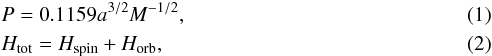 where
where  (3)and
 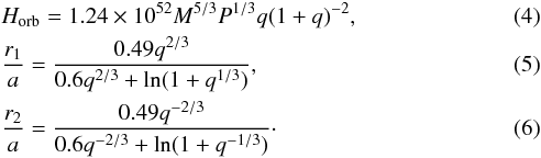 Here M = M1 + M2 is the total mass of the binary, Htot, Hspin, and Horb are total, rotational and orbital AM,
  and
and  are the (nondimensional) gyration radii of the components, r1 and r2 are the sizes of the inner Roche lobes, and q = M1/M2 is the mass ratio. Mass, radius, and semi-major axis are given in solar units, period in days, and AM in cgs units.
We assume that orbital and rotational motions are fully synchronized throughout the whole evolution, i.e. that the rotational period of each component is always equal to the orbital period P. This assumption is very well founded for close binaries based on both observations and theoretical considerations: systems with P< 10 are fully synchronized (Abt 2002), and synchronization time for periods shorter than 2−3 d is of the order of 104−105 yr (Zahn 1989).
We consider the evolution of an isolated binary, not interacting dynamically with any other object. So, stellar winds from the two components and the mass transfer between them, are the dominant mechanisms of the orbit evolution. The winds carry away mass and AM according to the formulae
 Here Ṁ is in solar masses per year and dHtot/ dt is in g cm2 s-1 per year. The formulae are calibrated by the observational data of the rotation of single, magnetically active stars of different age, and empirically determined mass-loss rates of single, solar-type stars. Both formulae apply in a limiting case of a rapidly rotating star in the saturated regime. We note that they do not contain any free adjustable parameters. The constant in Eq. (7) is uncertain within a factor of 2 and that in Eq. (8) is uncertain to ±30% (Stȩpień 2006b; Wood et al. 2002). The model ignores any interaction between winds from the two components.
The evolutionary calculations are divided into three phases: from ZAMS to the Roche lobe overflow (RLOF) by the initially more massive component (henceforth donor), rapid, conservative mass exchange from the more to less massive component (henceforth accretor), and the last phase of a slow mass exchange resulting from nuclear evolution of the donor.
The present computations follow those described in Stȩpień & Kiraga (2015, please refer to that paper for additional details, assumptions etc.). However, a couple of modifications were introduced to increase accuracy and computational efficiency of the code. In particular, upon approaching the final evolutionary state, the time step was substantially shortened to avoid nonphysical period oscillations observed in some cases by Stȩpień & Kiraga (2015). Instead of Padova models (Girardi et al. 2000), the newer PARSEC models2 (Bressan et al. 2012) were used, which include up-to-date physics and cover a broader range of metallicities. Finally, for modeling of V209 and V228, we calculated our own evolutionary tracks using a procedure outlined in Sect. 4.1.
4. The search for progenitors of the investigated binaries
Equations from the previous section do not contain any free adjustable parameters, so after specifying helium (Y) and metal (Z) content, the initial masses of both components and the initial orbital period, the evolution of the binary is fully determined. Our task is to examine the initial parameters space until a model binary that fits observations is found. We note that the result of the search is not unique if the physical parameters of the observed binary, i.e. chemical composition, orbital period, masses, sizes, and luminosities of the components are only used for matching (Stȩpień 2011). Several model binaries with different values of the initial parameters can reproduce the observed values, but in each case a different time is needed to reach the agreement with the observations.
To demonstrate the nonuniqueness of the solution in a broader context, we computed three sets of models with initial mass ratios qinit = 0.94, 0.82, and 0.72; all of them with initial total mass Minit = 1.55 M⊙, and low metallicity Z = 0.001 characteristic of globular clusters (Minit was kept fixed, assuming that a progenitor of an exemplary binary with the final total mass close to 1.4 M⊙ was searched for). Each set contained 16 binaries with initial orbital periods of between 1.5 d and 3 d. In Set 1, the initial component masses were equal to (0.8, 0.75) M⊙; in Sets 2 and 3 − to (0.85, 0.7) and (0.9, 0.65) M⊙, respectively. We note that accounting for mass loss owing to the wind, the MS-lifetime of a 0.8 M⊙ star exceeds the age of the Universe, while that of 0.85 M⊙ and 0.9 M⊙ is shorter than the age of most GCs.
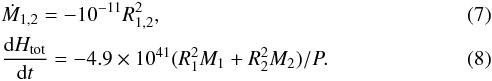
As it is seen in Fig. 1, the 0.8 M⊙ star fills its inner Roche lobe only in binaries with initial orbital periods shorter than 2.1 d. The orbits of these binaries are then so compact that soon afterwards both the components overfill the outer critical Roche surface and merge together. For periods equal to, or longer than 2.1 d, RLOF never occurs and the binaries stay detached. Set 1 models can only reproduce observed contact or near-contact binaries with parameters from a restricted range M1 ≲ 0.9 M⊙, M2 ≳ 0.55 M⊙ and P ≲ 0.4 d.
The situation changes a lot when we consider Set 2 binaries with M1 = 0.85 M⊙ (Fig. 2). An M1 = 0.85 M⊙ primary fills the Roche lobe during the MS evolutionary phase only in binaries with the four shortest periods. For all other periods, it leaves the main sequence while being detached from its Roche lobe, but the ensuing expansion quickly leads to the RLOF. A rapid mass exchange occurs, after which the orbital period increases and the mass ratio decreases. Set 2 models can reproduce observed binaries with parameters from a broad range M1 ≲ 1.25 M⊙,M2 ≳ 0.2 M⊙, and P from a fraction of a day up to a few days. Their final ages are concentrated around 11 Gyr. Figure 3 shows the evolution of Set 3 models with M1 = 0.9 M⊙. It is very similar to Fig. 2, except that the final ages are concentrated around 9 Gyr.
 |
Fig. 1 Time evolution of Set 1 models with initial component masses of 0.8 and 0.75 M⊙ (broken lines, left axis) and initial periods of 1.5−3.0 d (solid lines, right axis). Only the six shortest-period binaries reach the RLOF phase within the age of the Universe, enabling the mass exchange between their components. All other binaries stay detached. |
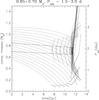 |
Fig. 2 Same as in Fig. 1 but for Set 2 models with initial component masses of 0.85 and 0.70 M⊙. Only the four shortest-period binaries enter the RLOF phase when the primary component is still on the main sequence. For all other binaries, RLOF occurs when the primary is past the main sequence i.e. at an age of ~11 Gyr. |
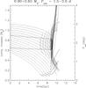 |
Fig. 3 Same as in Fig. 1 but for Set 3 models with initial component masses equal to 0.90 and 0.65 M⊙. Only the three shortest-period binaries enter the RLOF phase when the primary component is still on the main sequence. For all other binaries, RLOF occurs when the primary is past MS, i.e. at an age of ~9 Gyr. |
As we see, the final age of the model crucially depends on the initial mass of the primary, M1. Changing Z has a similar, but weaker effect to changing M1 (see Fig. 4). Knowledge of age and metallicity of the observed binary lifts the indeterminacy of the initial parameters. Fortunately, for GC members these parameters are known with a reasonable accuracy, even in clusters containing multiple subpopulations (Roediger et al. 2014).
Figures 1−3 may be regarded as an illustration of a coarse search of the parameter space. To reproduce the observed binary parameters more accurately, all three initial parameters have to be varied within a narrow range around the values resulting from the coarse search. This also includes the total initial mass because different component masses result in somewhat different mass losses. Examples of such fine search in period are shown in Figs. 5−8, which are related to the four actual binaries discussed below.
Data on observed and model binaries.
To select the best-fitting models, we applied the following procedure: first, we adopted the Y and Z parameters, in agreement with the observations of the parent clusters. Then, we evolved the model binary until the orbital period was to the third decimal place equal to that listed in Table 1, and, simultaneously, the observed component masses were reproduced within the observed uncertainties. This accuracy of period-fitting proved high enough for the resulting uncertainty of progenitor parameters to be negligible compared to the overall uncertainty dominated by sources discussed in the following sections. Finally, of all models meeting these criteria, the one with the age closest to the cluster age was selected. Radii, effective temperatures and luminosities of the components resulted automatically from the evolutionary sequences. The exception, discussed in detail in Sect. 4.1, were extremely low-mass stars (M< 0.2 M⊙) with helium cores and extended hydrogen envelopes, which we could not model reliably enough.
The basic data for the best-fitting models are given in Table 2. For each star, the left column contains the age of the parent cluster and the observed values of stellar parameters. The age of the model is given in the first row of the middle column and then all other parameters, as obtained from the model. For the secondary components of V209 and V8, no data on temperature and luminosity are given because we were not able to model extremely low-mass stars with a substantial helium core. A well known relation exists that connects the mass of the helium core with the stellar radius and luminosity, but it only applies to red giants with a sufficiently high total and core mass (Iben & Livio 1993; Eggleton 2009). Stars that are less massive than about 1 M⊙ with the helium core mass lower than about 0.2 M⊙ obey individual core mass-luminosity relation (see Fig. 2.9 in Eggleton 2009), as well as core mass-radius relation (Muslimov & Sarna 1996), depending on the total stellar mass. The right column gives for each star relative differences Δ(obs. − mod.) expressed in per cent.
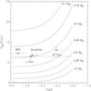 |
Fig. 4 Relation between metallicity and life-time on the MS for stars with different masses, based on PARSEC models. Indicated are the four clusters discussed in the present paper. Vertical and horizontal line segments give for each cluster uncertainties of both coordinates (see Table 1). |
The ages of V209 and V8 are close to the adopted ages of the hosting clusters ω Cen and NGC 6752, but a serious mismatch occurs in the remaining two cases, in which the best-fitting models are significantly younger than the corresponding clusters. The discrepancy is of a fundamental nature, as Fig. 4 shows. Here we plotted the MS lifetime of stars with different masses and metallicity. The lines of constant mass are shown with solid lines and labels. We also plotted the positions of all four clusters according to their age and metallicity. The positions give the maximum mass of a star which just reached TAMS in each cluster. This mass is close to, but not identical with, the turn-off mass. Specifically, the turn-off mass, defined as a hottest MS star on the isochrone corresponding to a given cluster, is lower by 0.01−0.02 M⊙ than the plotted maximum mass. Doubling this mass gives a good approximation of the maximum total mass of a close binary, which can still be found in the blue straggler region of the cluster (assuming a strictly conservative evolution, i.e. no mass loss from the system and no close interactions with other members of the cluster). The read-off values of the maximum mass are: 0.78 ± 0.01 M⊙ for M 55, 0.8−0.9 M⊙ for ω Cen, 0.80 ± 0.01 M⊙ for NGC 6752 and 0.81 ± 0.01 M⊙ for 47 Tuc. While the observed total masses of the analyzed binaries in ω Cen and NGC 6752 are lower than these limits, they are higher in two other clusters: 1.586 versus 1.56 M⊙ for M 55, and 1.712 versus 1.62 M⊙ for 47 Tuc. Moreover, the evolutionary model includes the mass loss of several percent during the binary evolution (mostly during the longest first phase), so the initial component masses must be even higher than the measured ones (see Table 2). In effect, no model binary can be found that reproduces the observed total mass and age of V60 and V228 (assuming, of course, that their ages are equal to the ages of their parent clusters).
4.1. V209
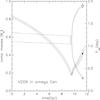 |
Fig. 5 Time variations of orbital period (solid lines, right axis) and component masses (broken lines, left axis) of the best fitting model of V209 (see Table 2 for its initial parameters). Also shown are two models with the same initial component masses, and periods differing by ±0.02 d from the best-fitting one. The observed parameters of V209 are indicated by a filled circle (period) and diamonds (masses). Vertical sizes of the diamonds correspond to observational errors. |
ω Cen is the most massive but also the most unusual GC in our Galaxy. It shows a very complex structure with a very broad MS, suggestive of a combination of a few independent sequences, multiple horizontal, subgiant and red giant branches, and a large spread in heavy element content (Norris et al. 1997; Johnson et al. 2010; Piotto et al. 2005; Joo & Lee 2013; Fraix-Burnet & Davoust 2015, and references therein). As a result, several (up to seven) different subpopulations have been identified with different chemical compositions and ages. In particular, an enhanced helium abundance was suggested for two subpopulations (Joo & Lee 2013; Fraix-Burnet & Davoust 2015).
To find a progenitor of V209, we first used PARSEC models in a search for desirable initial binary parameters. It quickly turned out that at the helium abundance Y = 0.25−0.27 the primary of V209 is far too hot for its mass, independently of metal content and age varying within the observed values. It is known, however, that evolutionary tracks of the helium enriched models are shifted towards higher temperatures (and higher luminosities) in the CMD, compared to normal helium abundance models (Glebbeek et al. 2010). Based on the suggestion that a significant subpopulation of cluster members may have helium content Y ≈ 0.40 (Joo & Lee 2013; Fraix-Burnet & Davoust 2015), we generated our own grid of evolutionary tracks for helium-enriched stars.
The tracks were computed using the Warsaw-New Jersey evolution code, which is an updated version of B. Paczyński’s code (Paczyński 1969, 1970). The computations were performed starting from chemically uniform models on the ZAMS. The input parameters for evolutionary model sequences are total mass, M, initial value for helium abundance, Y0, and heavy element abundance, Z. We computed two series of models with masses from 0.50 to 1.60 M⊙, with a step size of 0.05 M⊙. In one series of the computations, we assumed Y0 = 0.40,Z = 0.0004, in the second one, −Y0 = 0.27,Z = 0.003. For chemical elements heavier than helium, we adopted the solar element mixture of Asplund et al. (2009). For the opacities, we used the Opacity Project (OP) data (Seaton 1996, 2005) supplemented at log T< 3.95 with the low-temperature data of Ferguson et al. (2005). In all computations, the OPAL equation of state was used (Rogers et al. 1996, version OPAL EOS 2005). The nuclear reaction rates are the same as used by Bahcall & Pinsonneault (1995). In the stellar envelope, the standard mixing-length theory of convection with the mixing-length parameter α = 1.6 was used. The choice of the mixing-length parameter is important in our models because they are sufficiently cold to have an effective energy transfer by convection in the stellar envelope, namely in the regions of partial ionization of hydrogen and helium, and therefore will have an influence on the structure of the models and their position on the HR diagram. We used a value of α to be close to estimations for the Sun between 1.7 and 2.0 (Magic et al. 2015), as obtained from 3D computations and calibration to the solar radius.
Based on those models, we were able to find a progenitor of V209 (see Table 2). A binary with the initial orbital period of 1.66 d and the component masses of 0.65 and 0.55 M⊙ evolves after 11.34 Gyr (which is almost equal to the adopted age of ω Cen) into a binary with parameters close to V209, see Fig. 5. Tracks for two additional models are also plotted to illustrate the accuracy of the fine parameter search, in this case in period. The models have the same initial component masses as the best-fitting one, but their initial periods differ by ±0.02 d from the best-fitting one. The obs. − mod. differences are significantly larger for them: ΔP = 0.8% and 6.8%, ΔM1 = 3.7% and 0.1% and ΔM2 = 8% and 13% for the shorter and longer period model, respectively. A change of either component mass by, for example, 1% results in a similar worsening of the fit. We conclude that fitting the model to the observations with the assumed accuracy requires a really fine tuning of the initial parameters.
We note that, in our model, unlike in the scenario proposed by Kaluzny et al. (2007a), there is no need for the binary to experience two CE phases: just one mass transfer phase is sufficient to reproduce all the observed parameters of the primary (accretor) within the observational uncertainty. Unfortunately, in the case of the secondary (donor), we could only compute its mass and the mass of its helium core. We followed the evolution of the donor until its mass approached 0.2 M⊙, assuming that it still fills its Roche lobe. The helium core then reached a mass of about 0.13 M⊙. As the mass of the star decreases beyond 0.2 M⊙ , its radius shrinks rapidly, the star detaches from the Roche lobe, and loses mass via stellar wind and during the thermonuclear flashes that occur in the hydrogen burning shell (Sarna & De Greve 1996; Muslimov & Sarna 1996; Driebe et al. 1998; Althaus et al. 2013). Below about 0.18 M⊙, flashes disappear but the radius (and mass) continues to decrease as the star moves to the high temperature region in the HR diagram. These phases are not described by our model because of a lack of sufficiently dense grid of evolutionary models of these types of stars. Nevertheless, the precise fit of our model to the observed parameters of the primary component of V209, in particular an unusually high effective temperature for its mass, may be regarded as independent and strong evidence for the existence of a stellar subpopulation in ω Cen with the high helium content of Y = 0.40.
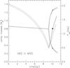 |
Fig. 6 Same as in Fig. 5, but for V60 in M 55. The two additional models have initial periods differing by ±0.025 d from the best-fitting one. |
4.2. V60
This binary was already used by Stȩpień & Kiraga (2015) to demonstrate the potential of the method that was outlined in Sect. 3 in identifying progenitors of close binaries in GCs. Among models calculated in that paper, the one with Pinit = 1.9 d and component masses (M1,M2) = (0.89, 0.80) M⊙ reproduced the observed parameters of V60 fairly well. However, it could not be regarded as a solution to the present problem since its metallicity did not conform to the limits given in Table 2, and, moreover, the whole BS population of Stȩpień & Kiraga (2015) was generated without paying attention to the age of the models. Thus, a standard search of the parameter space was necessary. Once finished, we found that the model that best matches the present values P,M1, and M2 was over 2 Gyr younger than M 55. As argued at the beginning of Sect. 4, this discrepancy is a direct consequence of the doubled turn-off mass of M 55 being smaller than the total mass of V60. The results of the present fit are shown in Fig. 6.
The CMD of the cluster suggests a presence of subpopulations that differ in age and/or chemical composition (Piotto et al. 2015). An age discrepancy of 2 Gyr between them seems rather unlikely, but it can not be entirely excluded. On the other hand, the ages of M 55 and V60 could be reconciled if the metallicity of the straggler were significantly higher than the upper limit given in Table 2. Figure 4 shows that the present total mass of V60 can be reached for Z ≈ 0.005, i.e. about 15 times higher than obtained for the cluster (we note that M 55 is the most metal-poor of all the GCs discussed in this paper). If V60 belonged to a subpopulation younger by 1 Gyr than the cluster, the value of Z necessary for the turn-off mass to be equal to the total mass of the binary would decrease to 0.003, a value that is still much larger than observed. Clearly, more data and better models are needed to resolve the discrepancy.
4.3. V228
This is another variable star for which a substantial discrepancy occurs between the adopted age of the cluster and the age of the best fitting model (Table 2 and Fig. 7). The PARSEC models with the metallicity of 0.003 are not available, so we decided to compute a special set of models with this value of Z and a helium content Y = 0.27. The best fitting model has the initial component masses equal to 0.95 and 0.94 M⊙, orbiting each other with the period of 2.129 d.
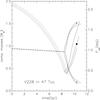 |
Fig. 7 Same as in Fig. 5, but for V228 in 47 Tuc. The two additional models have initial periods differing by −0.02 and 0.04 d from the best-fitting one. |
A binary with a total mass this large, and metallicity characteristic of 47 Tuc, should be past the red giant phase long before the age of the cluster. Here, the discrepancy between the cluster and model age is even larger than for M 55 (2.7 vs. 2.1 Gyr). Similar to other clusters, 47 Tuc also shows multiple subpopulations (Joo & Lee 2013; Piotto et al. 2015), but so far no data on the age spread are available. Alternatively, the age of the model binary can be brought to agreement with the cluster age if its components have metallicity 3−4 times higher than adopted for the cluster.
The secondary of V228 reached a mass of 0.2 M⊙ , but it still fills its Roche lobe and has characteristics of a subgiant with a helium core of 0.12−0.13 M⊙. The model reproduces the observed parameters quite well. We expect the star to detach soon from its Roche lobe and to move to the left in the HR diagram. The agreement of the model with the primary of V228 is somewhat poorer. In particular, the radius of the accretor is significantly larger than observed, and also the temperature is significantly higher. As a result, the luminosity of the model primary is too high by 0.19 dex, compared to the observations. The difference suggests that the real primary is less evolutionarily advanced than the model.
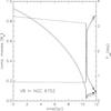 |
Fig. 8 Same as in Fig. 5, but for V8 in NGC 6752. The two additional models have initial periods differing by ±0.025 d from the best-fitting one. |
4.4. V8
This is the most unusual binary system of all discussed in the present paper. It is a near contact binary with an extremely low mass secondary of 0.12 M⊙ , which possesses the radius of 0.45 R⊙ and fills its Roche lobe. A single star with this mass and a significant helium core has a much lower radius as the calculations by Muslimov & Sarna (1996) show. A similarly low radius results from the paper by Paczyński et al. (2007) who computed radii of several stars with masses between 0.18−0.14 M⊙ and different helium cores. The maximum stellar radius decreases from about 1.3 R⊙ for a 0.18 M⊙ star down to about 0.3 R⊙ for a 0.14 M⊙ star. An extrapolation of this trend to 0.12 M⊙ gives a maximum radius of about 0.15 R⊙, in good agreement with the paper by Muslimov & Sarna (1996). The observed large value of the radius must result from the interaction with the other component. V8 may remind us in this respect of AW UMa (Rucinski 2015), where the 0.13 M⊙ secondary possesses a massive helium core and is submerged in the matter flowing from the 1.3 M⊙ primary component. AW UMa looks like a typical contact system of W UMa-type with the secondary radius of about 0.5 R⊙, yet the detailed observations of this binary obtained by Rucinski (2015) indicate a much more complex geometry of the system, where both components do not actually fill their Roche lobes, but are surrounded by the equatorial flow extending up to the inner critical surface. The existence of this type of flow in contact and near contact binaries was predicted by Stȩpień (2009) and Stȩpień & Kiraga (2013). The flow redistributes energy between the components, resulting in an apparent equality of their effective temperatures, which we also see in V8 (see Table 2).
The observational parameters of V8 result from the solution of the light curve only. No radial velocity curve exists for the variable, which makes the solution rather uncertain. Fortunately, one of the eclipses is total so the range of likely parameter values is not too large. The best fitting model has the values of the main parameters satisfactorily close to the observed ones (see Table 2 and Fig. 8), but the radius and temperature of the accretor are significantly lower than observed. This results most likely from the fact that the donor transferred to the accretor not only its outer layers with the original hydrogen content, but also an amount of matter enriched in helium by the nuclear reactions. As a result, the accretor behaves like a more evolutionarily advanced star, compared to the model. Our simple modeling procedure does not take this into account. It assumes that all the transferred matter is hydrogen-rich so after the mass transfer the accretor has the hydrogen content very close to that of a zero age MS star.
The discrepancy is closely related to another caveat of the best fitting model. To satisfactorily reproduce the observed parameters, it was necessary to assume an initial mass ratio qinit = M1,init/M2,init = 4.47. During the rapid mass transfer after RLOF, the orbital period decreased to about 0.1 d, which resulted in the overflow of the outer critical Roche surface by the common stellar surface. The assumption of the conservative mass transfer very likely breaks down in this case. However, to allow for the nonconservative mass transfer, two additional free parameters describing the amount of mass and AM lost from the system would be necessary. Because we avoid this, the conservative mass transfer can be considered as a limiting case when all the matter from the CE ultimately returns to the stars. We note, that the model of V8 is the only one with such an extreme initial mass ratio.
5. Discussion
We have reproduced the present configurations of the considered systems, assuming a conservative evolution of isolated binaries (apart from the mass and AM loss by stellar winds). Obviously, this result does not prove that V209, V60, V228, and V8 are formed in this way but just indicates such a possibility. Approximating the evolution of binary components with single star models only works well in case of V209. While, for the remaining three BSs, orbital periods and component masses also agree with observations, radii, and temperatures derived from modeling differ from the observed ones by several standard deviations. This points to the limitations of the simple evolutionary code employed in this paper. A sequence of evolutionary models of single stars correctly describes the evolution of close binary components only until the rapid mass exchange. Later on, the evolution of both components deviates increasingly from that of single stars, in particular when the accretor begins to receive nuclearly processed matter from the deeper layers of the donor. An obvious improvement would be to replace the present code with a binary evolution code, solving the equations of the internal structure of each component at every time step, and allowing for the mass transfer between the components. The next step would be to incorporate the dynamical processes that take place in close binaries, but are still poorly understood, like the rapid mass transfer following RLOF with an unknown amount of mass and AM lost from the system (Sarna & De Greve 1996), or the mass flow carrying thermal energy from the primary to secondary component in a contact binary (Stȩpień 2009; Rucinski 2015).
The BS progenitors identified in the present survey are close binaries. Below we argue that this result is calculationally robust, and physically feasible.
Uncertainties in the evolutionary modeling procedure outlined in Sect. 3 are discussed in detail by Stȩpień & Kiraga (2015). Here we only make use of their most important conclusions. The progenitors of V209, V60, V228, and V8 have lost, respectively, ΔM = 7.7%, 8.8%, 9.7% and 7.8%, and ΔAM = 67%, 53%, 72% and 71%. An increase of the mass loss rate by a factor of 2 entails an increase of M by ΔM, whereas its decrease by 50% entails a decrease of M by ΔM/2. Similarly, decreasing/increasing the AM loss rate by 30% requires a decrease/increase of the initial AM by the same percentage of ΔAM, which corresponds to initial orbital periods of 0.84 and 2.88 d for V209, 1.30 and 3.03 d for V60, 1.63 and 2.71 d for V228, and 2.82 and 3.71 d for V8 (calculated for M kept constant).
Thus, varying the coefficients in Eqs. (7) and (8) within observationally acceptable limits cannot cause the model progenitors to leave the short-period regime.
The next question to ask is: can close binaries be sufficiently abundant in a GC to account for the observed binary BSs? The efficient tightening of binaries in triple systems by the Kozai mechanism can be mentioned in this respect. The presence of a third body stimulates the so-called Kozai cycles which, together with the tidal energy dissipation, can shorten an orbital period of 1−2 weeks down to a couple of days within less than 108 yr (Eggleton & Kiseleva-Eggleton 2006; Fabrycky & Tremaine 2007; Naoz & Fabrycky 2014). If this is the principal source of close binaries in GCs, then a local maximum around 2−4 days may be expected in the period distribution of young cluster binaries, similar to that observed by Tokovinin & Smekhov (2002) among spectroscopic subsystems of visual multiple stars. Close binaries can also be formed due to so called hardening encounters with single or binary cluster members (see for example Leigh et al. 2015, and references therein). We note that the progenitors do not have to be formed as close binaries; it is sufficient for them to tighten shortly before the more massive component leaves the main sequence, so that there is ample time for the hardening to occur. However, the recent research of Hypki & Giersz (2016) suggests that most of the evolutionary BSs result from the unperturbed evolution of primordial binaries.
Whether primordial or hardened, all the four binaries considered here have experienced a rapid mass exchange with the mass-ratio reversal. Their present primaries are main-sequence objects substantially enriched in matter from the companion. An exception is V60, whose primary is still accreting, and may be quite far from thermal equilibrium (Rozyczka et al. 2013). The secondaries are evolutionarily advanced objects with considerable helium cores. Two of them are already heading towards the sdB domain, and the third one (in V228) should do it soon. The most probable scenario for the ultimate fate of all the four systems involves the CE phase beginning when the present primaries reach the RGB, and followed either by a merger (Tylenda et al. 2011; Stȩpień & Kiraga 2015) or the formation of a close binary with two degenerate stars.
The good agreement between the ages of V209 and V8 and the ages of their parent clusters does not exclude the possibility that they were formed after the bulk of the cluster. Assuming, for example, that V209 should belong to a younger subpopulation, it is possible to slightly increase the initial mass of the donor and to accordingly modify the mass of the other component together with the initial orbital period, so that the evolutionary time-scale of the binary will be shorter. Similarly, the age of model (4) describing V8 can be altered by an appropriate modification of the donor mass as is demonstrated in Figs. 1−3.
Binaries V60 and V228 are apparently younger than M 55 and 47 Tuc or, in other words, are overmassive for the ages of their parent clusters. While it is tempting to suggest that they are members of younger subpopulations, it would be premature to do so. First, it is conceivable that overmassive systems are products of multiple mergers or collisions (Sandquist et al. 2003; Leigh & Sills 2011). Second, as we argue in the following paragraphs, available stellar evolution models are simply not reliable enough to draw such far-reaching conclusions. In particular, an apparent age discrepancy may emerge whenever MS life-times of models applied to determine the age of the cluster differ from those of models applied to evolve individual binaries. We note, however, that the cases of V60 and V228 are not unique. Based consistently on Dartmouth evolutionary models, Kaluzny et al. (2015b) found that the detached main-sequence binaries V40 and V41 in NGC 6362 differ in age by 1.3 ± 0.4 Gyr, i.e. statistically significant at the 3σ level. In our opinion, all these discrepancies are vexing enough to be closely examined by more accurate observations and better modeling.
A broader context of our findings is origin and evolution of GCs. Obtaining the absolute age of a cluster involves many steps in transformation of observational data into theoretical parameters to which models can be fitted. Both the poor data and oversimplified theory may generate incoherent results or even paradoxes, like cluster ages significantly exceeding the Hubble time. The latter values were still being derived in the late 90 s, as emphasized by VandenBerg (2000), who thoroughly rediscussed the issue and obtained ages between 8 and 14 Gyr. While the basic paradox had been removed, the problem is far from settled. Although new methods of age determination have been introduced, in addition to the original isochrone fitting, all of them remain strongly model-dependent, be it sophisticated isochrone construction (Dotter 2016) or comparing absolute parameters of turn-off stars or detached binaries with the output of stellar evolution codes (Marín-Franch et al. 2009, project CASE, see Introduction). Moreover, in spite of constant progress in modeling significant differences exist among codes used by different authors. Important physical processes like convection, semiconvection, diffusion, mixing, or rotation are usually described by single-value parameters that are adopted individually in each code. Cool, solar-type stars generate winds induced by their magnetic activity, but the resulting mass and AM loss has been largely neglected when computing evolutionary tracks. Only very recently some codes, like MESA, have included such losses as an option.
Even Y and Z – the fundamental parameters describing the chemical composition of a star – do not always have a well-defined meaning, since the [Fe/H] index, which is often used as an input parameter, may relate to different values of Z⊙. Moreover, different transformations [Fe/H] → Z may be used, and different correlations between Z and Y may be assumed. No wonder that the resulting stellar parameters differ from one code to another. The codes are typically calibrated on the Sun, so they reproduce MS solar type stars in a consistent way. Yet, the most important parameter for the correct determination of GC ages, i.e. MS life-time can differ for some stars quite considerably. To give an example, the old Padova model of a 0.8 M⊙ star with Z = 0.001 has MS life time equal to 13.5 Gyr (Girardi et al. 2000), whereas the new PARSEC model of the same star only 11.95 Gyr (Bressan et al. 2012). Another example: recently published by Lagarde et al. (2012) 0.85 M⊙ model with Z = 0.0001 has the MS life of 11.14 Gyr, compared to 9 Gyr for the PARSEC model with the same Z. Differences in time-scales between models beyond the MS are still greater. This diversity recently concerned a number of authors who discuss the influence of several physical mechanisms on models produced by different codes and compare them to well calibrated observational data (Nataf et al. 2012; Martins & Palacios 2013; Ghezzi & Johnson 2015; Meynet et al. 2016; Stancliffe et al. 2015; Valle et al. 2016b,a). However, uncertainties of stellar evolution models still remain the primary factor that impedes the accurate determination of the absolute ages of globular clusters. Observational uncertainties will dramatically decrease when Gaia parallaxes become available (distances to many GCs will be known with an accuracy better than one per cent; Pancino et al. 2013). If the theory is to catch up with observations, much more effort in exposing and diagnosing its problems is needed. We believe that evolutionary simulations of binary blue stragglers is a very useful tool to achieve this goal.
6. Conclusions
-
1.
The results of the present investigation demonstrate animportance of the close binary evolution in the formation of bluestragglers. In particular, it was shown that blue stragglers resultfrom rejuvenation of an initially less massive component that isfed by the hydrogen rich matter from its companion overflowingthe inner Roche lobe.
-
2.
To reproduce the present parameters of V209 in ω Cen, it was necessary to adopt the increased helium content Y = 0.40 of this binary. This is further evidence in favour of the existence of the helium-rich subpopulation in this cluster.
-
3.
The best fitting models of V60 in M 55 and V228 in 47 Tuc are too massive for the age of the parent cluster as it is currently estimated. Unless this is an apparent effect resulting from an inconsistency between models used for GC age determination and binary modeling, these systems may belong to younger subpopulations or may result from dynamical multibody interactions.
-
4.
Different evolutionary codes produce mutually inconsistent stellar parameters. A better description of physical processes influencing the stellar evolution is urgently needed. Until this shortage is overcome, the absolute age determination of globular clusters will be plagued with substantial uncertainties.
-
5.
Studying the evolution of binary BSs in GCs emerges as a new research tool that provides an independent insight into interactions between GC members and enables sensitive tests of stellar evolution codes.
Acknowledgments
This paper is dedicated to the memory of Janusz Kaluzny, founder and long-time leader of CASE, who prematurely passed away in March 2015. We thank an anonymous referee for very insightful remarks that significantly improved the final shape of the paper. A.A.P. acknowledges partial support from the Polish National Science Center (NCN) grant 2015/17/B/ST9/02082. M.R. was supported by the NCN grant DEC-2012/05/B/ST9/03931.
References
- Abt, H. A. 2002, ApJ, 573, 359 [NASA ADS] [CrossRef] [Google Scholar]
- Althaus, L. G., Miller Bertolami, M. M., & Coŕsico, A. H. 2013, A&A, 557, A19 [NASA ADS] [CrossRef] [EDP Sciences] [Google Scholar]
- Asplund, M., Grevesse, N., Sauval, A. J., & Scott, P. 2009, ARA&A, 47, 481 [NASA ADS] [CrossRef] [Google Scholar]
- Bahcall, J. N., & Pinsonneault, M. H. 1995, Rev. Mod. Phys, 67, 781 [NASA ADS] [CrossRef] [Google Scholar]
- Bressan, A., Marigio, P., Girardi, L., et al. 2012, MNRAS, 427, 127 [NASA ADS] [CrossRef] [Google Scholar]
- Cannon, R. D. 2015, in Ecology of Blue Straggler Stars (Berlin, Heidelberg: Springer-Verlag), Astrophys. Space Sci. Lib., 413, 17 [CrossRef] [Google Scholar]
- Chatterjee, S., Rasio, F. A., Sills, A., & Glebbek, E. 2013, ApJ, 777, 106 [NASA ADS] [CrossRef] [Google Scholar]
- Chen, X., & Han, Z. 2008, MNRAS, 384, 1263 [NASA ADS] [CrossRef] [Google Scholar]
- Dotter, A. 2016, ApJS, 222, 8 [NASA ADS] [CrossRef] [Google Scholar]
- Driebe, T., Schonberger, D., Blocekr, T., & Herwig, F. 1998, A&A, 339, 123 [NASA ADS] [Google Scholar]
- Eggleton, P. P. 1983, ApJ, 268, 368 [NASA ADS] [CrossRef] [Google Scholar]
- Eggleton, P. 2006, Evolutionary Processes in Binary and Multiple Stars, (Cambridge: Cambridge Univ. Press) [Google Scholar]
- Eggleton, P. P., & Kiseleva-Eggleton, L. 2006, Astrophys. Space Phys. Res., 304, 74 [Google Scholar]
- Fabrycky, D., & Tremaine, S. 2007, ApJ, 669, 1298 [NASA ADS] [CrossRef] [Google Scholar]
- Ferguson, J. W., Alexander, D. R., Allard, F., et al. 2005, ApJ, 623, 585 [NASA ADS] [CrossRef] [Google Scholar]
- Ferraro, F. R., Lanzoni, B., Dalessandro, E., et al. 2012, Nature, 492, 393 [NASA ADS] [CrossRef] [Google Scholar]
- Ferraro, F. R., Lanzoni, B., Dalessandro, E., Mucciarelli, A., & Lovisi, L. 2015, Ecology of Blue Straggler Stars (Berlin, Heidelberg: Springer-Verlag), Astrophys. Space Sci. Lib., 413, 99 [CrossRef] [Google Scholar]
- Forbes, D. A., & Bridges, T. 2010, MNRAS, 404, 1203 [NASA ADS] [Google Scholar]
- Fraix-Burnet, D., & Davoust, E. 2015, MNRAS, 450, 3431 [NASA ADS] [CrossRef] [Google Scholar]
- Gazeas, K., & Stȩpień, K. 2008, MNRAS, 390, 1577 [NASA ADS] [Google Scholar]
- Ghezzi, L., & Johnson, J. A. 2015, ApJ, 812, 96 [NASA ADS] [CrossRef] [Google Scholar]
- Girardi, L., Bressan, A., Bertelli, G., & Chiosi, C. 2000, A&AS, 141, 371 [NASA ADS] [CrossRef] [EDP Sciences] [Google Scholar]
- Glebbeek, E., Sills, A., & Leigh, N. 2010, MNRAS, 408, 1267 [NASA ADS] [CrossRef] [Google Scholar]
- Harris, W. E. 1996, AJ, 112, 1487 (2010 edn.) [NASA ADS] [CrossRef] [Google Scholar]
- Hills, J. G., & Day, C. A. 1997, Astrophys. Lett., 17, 87 [Google Scholar]
- Hypki, A., & Giersz, M. 2013, MNRAS, 4219, 1221 [NASA ADS] [CrossRef] [Google Scholar]
- Hypki, A., & Giersz, M. 2016, MNRAS, submitted [arXiv:1604.07033] [Google Scholar]
- Iben, I., & Livio, M. 1993, PASP, 105, 1373 [Google Scholar]
- Johnson, C. I., & Pilachowski, C. A. 2010, ApJ, 772, 1373 [NASA ADS] [CrossRef] [Google Scholar]
- Lagarde, N., Decressin, T., Charbonnel, C., et al. 2012, A&A, 543, A108 [NASA ADS] [CrossRef] [EDP Sciences] [Google Scholar]
- Joo, S.-J., & Lee, Y.-W. 2013, ApJ, 762, 36 [NASA ADS] [CrossRef] [Google Scholar]
- Kaluzny, J., Kubiak, M., Szymański, M., et al. 1996, A&AS, 120, 139 [NASA ADS] [CrossRef] [EDP Sciences] [Google Scholar]
- Kaluzny, J., Kubiak, M., Szymański, M., et al. 1998, A&AS, 128, 19 [NASA ADS] [CrossRef] [EDP Sciences] [Google Scholar]
- Kaluzny, J., Thompson, I. B., Krzeminski, W. et al. 2005, in Stellar Astrophysics with the World’s Largest Telescopes, AIP Conf. Proc., 752, 70 [Google Scholar]
- Kaluzny, J., Ruciński, S. M., Thompson, I. B., Pych, W., & Krzemiński, W. 2007a, AJ, 133, 2457 [NASA ADS] [CrossRef] [Google Scholar]
- Kaluzny, J., Thompson, I. B., Ruciński, S. M., et al. 2007b, AJ, 134, 541 [NASA ADS] [CrossRef] [Google Scholar]
- Kaluzny, J., Rozyczka, M., Thompson, I. B., & Zloczewski, K. 2009, Acta Astron., 59, 371 [NASA ADS] [Google Scholar]
- Kaluzny, J., Thompson, I. B., Krzemiński, W., & Zloczewski, K. 2010, Acta Astron., 60, 245 [NASA ADS] [Google Scholar]
- Kaluzny, J., Thompson, I. B., Rozyczka, M., & Krzemiński, W. 2013a, Acta Astron., 63, 181 [NASA ADS] [Google Scholar]
- Kaluzny, J., Rozyczka, M., Pych, W., et al. 2013b, Acta Astron., 63, 309 [NASA ADS] [Google Scholar]
- Kaluzny, J., Thompson, I. B., Rozyczka, M., Pych, W., & Narloch, W. 2014, Acta Astron., 64, 309 [NASA ADS] [Google Scholar]
- Kaluzny, J., Thompson, I. B., Narloch, W., Pych, W., & Rozyczka, M. 2015a, Acta Astron., 65, 267 [NASA ADS] [Google Scholar]
- Kaluzny, J., Thompson, I. B., Dotter, A., et al. 2015b, AJ, 150, 155 [NASA ADS] [CrossRef] [Google Scholar]
- Kaluzny, J., Rozyczka, M., Thompson, I. B., et al. 2016, Acta Astron., 66, 31 [NASA ADS] [Google Scholar]
- Kayser, A., Hilker, M., Richtler, T., & Willemsen, P. G. 2006, A&A, 458, 777 [NASA ADS] [CrossRef] [EDP Sciences] [Google Scholar]
- Lapenna, E., Lardo, C., Mucciarelli, A., et al. 2016, A&AS, 120, 139 [Google Scholar]
- Leigh, N., & Sills, A. 2011, MNRAS, 410, 2370 [NASA ADS] [CrossRef] [Google Scholar]
- Leigh, N., Giersz, M., Marks, M., et al. 2015, MNRAS, 446, 226 [NASA ADS] [CrossRef] [Google Scholar]
- Magic, Z., Weiss, A., & Asplund, M. 2015, A&A, 573, A89 [NASA ADS] [CrossRef] [EDP Sciences] [Google Scholar]
- Marín-Franch, A., Aparicio, A., Piotto, G., et al. 2009, ApJ, 694, 1498 [NASA ADS] [CrossRef] [Google Scholar]
- Marino, A. F., Milone, A. P., Casagrande, L., et al. 2016, MNRAS, 459, 610 [NASA ADS] [CrossRef] [Google Scholar]
- Martins, F., & Palacios, A. 2013, A&A, 560, A16 [NASA ADS] [CrossRef] [EDP Sciences] [Google Scholar]
- McCrea, W. H. 1964, MNRAS, 128, 147 [NASA ADS] [CrossRef] [Google Scholar]
- Meynet, G., Maeder, A., Eggenberger, P., et al. 2016, Astron. Nachr., 337, 8 [CrossRef] [Google Scholar]
- Muslimov, A., & Sarna, M. J. 1996, ApJ, 464, 867 [NASA ADS] [CrossRef] [Google Scholar]
- Naoz, S., & Fabrycky, D. C. 2014, ApJ, 793, 137 [NASA ADS] [CrossRef] [Google Scholar]
- Nataf, D. M., Gould, A., & Pinsonneault, M. H. 2012, Acta Astron., 62, 33 [NASA ADS] [Google Scholar]
- Norris, J. E., Freeman, K. C., Mayor, M., & Seitzer, P. 1997, ApJ, 487, L187 [NASA ADS] [CrossRef] [Google Scholar]
- Paczyński, B. 1969, Acta Astron., 19, 1 [NASA ADS] [Google Scholar]
- Paczyński, B. 1970, Acta Astron., 20, 47 [NASA ADS] [Google Scholar]
- Paczyński, B., Sienkiewicz, R., & Szczygieł, D. M. 2007, MNRAS, 378, 961 [NASA ADS] [CrossRef] [Google Scholar]
- Pancino, E., Rejkuba, M., Zoccali, M., & Carrera, R. 2010, A&A, 524, A44 [NASA ADS] [CrossRef] [EDP Sciences] [Google Scholar]
- Pancino, E., Bellazzini, M., & Marinoni, S. 2013, Mem. Soc. Astron. It., 75, 282 [Google Scholar]
- Perets, H. B. 2015, in Ecology of Blue Straggler Stars (Berlin, Heidelberg: Springer-Verlag), Astrophys. Space Sci. Lib., 413, 251 [CrossRef] [Google Scholar]
- Piotto, G., De Angeli, F., King, I. R., et al. 2004, ApJ, 604, 109 [Google Scholar]
- Piotto, G., Villanova, S., Bedin, L. R., et al. 2005, ApJ, 621, 777 [NASA ADS] [CrossRef] [Google Scholar]
- Piotto, G., Milone, A. P., Bedin, L. R., et al. 2015, AJ, 149, 91 [NASA ADS] [CrossRef] [Google Scholar]
- Roediger, J. C., Courteau, S., Graves, G., & Schiavon, R. P. 2014, ApJS, 210, 10 [Google Scholar]
- Rogers, F. J., Swenson, F. J., & Iglesias, C. A. 1996, ApJ, 456, 902 [NASA ADS] [CrossRef] [Google Scholar]
- Rozyczka, M., Kaluzny, J., Thompson, I. B., et al. 2013, Acta Astron., 63, 67 [NASA ADS] [Google Scholar]
- Rucinski, S. M. 2015, AJ, 149, 49 [NASA ADS] [CrossRef] [Google Scholar]
- Sandage, A. 1953, AJ, 58, 61 [NASA ADS] [CrossRef] [Google Scholar]
- Sandquist, E. L., Latham, D. W., Shetrone, M. D., & Milone, A. A. E. 2003, AJ, 125, 810 [NASA ADS] [CrossRef] [Google Scholar]
- Sarna, M. J., & De Greve, J.-P. 1996, QJRAS, 37, 11 [NASA ADS] [Google Scholar]
- Seaton, M. J. 1996, MNRAS, 279, 95 [NASA ADS] [CrossRef] [Google Scholar]
- Seaton, M. J. 2005, MNRAS, 362, L1 [NASA ADS] [CrossRef] [Google Scholar]
- Shara, M. M., Saffer, R. A., & Livio, M. 1997, ApJ, 489, L59 [NASA ADS] [CrossRef] [Google Scholar]
- Stancliffe, R. J., Fossati, L., Passy, J.-C., & Schneider, F. R. N. 2015, A&A, 575, A117 [NASA ADS] [CrossRef] [EDP Sciences] [Google Scholar]
- Stȩpień, K. 2006a, Acta Astron., 56, 199 [NASA ADS] [Google Scholar]
- Stȩpień, K. 2006b, Acta Astron., 56, 347 [NASA ADS] [Google Scholar]
- Stȩpień, K. 2009, MNRAS, 397, 857 [NASA ADS] [CrossRef] [Google Scholar]
- Stȩpień, K. 2011, Acta Astron., 61, 139 [NASA ADS] [Google Scholar]
- Stȩpień, K., & Kiraga, M. 2013, Acta Astron., 63, 239 [NASA ADS] [Google Scholar]
- Stȩpień, K., & Kiraga, M. 2015, A&A, 577, A117 [NASA ADS] [CrossRef] [EDP Sciences] [Google Scholar]
- Thompson, I. B., Kaluzny, J., Pych, W., & Krzeminski, W. 1999, AJ, 118, 462 [NASA ADS] [CrossRef] [Google Scholar]
- Tokovinin, A. A., & Smekhov, M. G. 2002, A&A, 382, 118 [NASA ADS] [CrossRef] [EDP Sciences] [Google Scholar]
- Tylenda, R., Hajduk, M., Kamiński, T., et al. 2011, A&A, 528, A114 [Google Scholar]
- Valle, G., Dell’Omodarme, M., Prada Moroni, P. G., & Degl’Innocenti, S. 2016a, A&A, 587, A31 [NASA ADS] [CrossRef] [EDP Sciences] [Google Scholar]
- Valle, G., Dell’Omodarme, M., Prada Moroni, P. G., & Degl’Innocenti, S. 2016b, A&A, 587, A16 [NASA ADS] [CrossRef] [EDP Sciences] [Google Scholar]
- VandenBerg, D. A. 2000, ApJS, 129, 315 [NASA ADS] [CrossRef] [Google Scholar]
- Wood, B. E., Müller, H. R., Zank, G. P., & Linsky, J. L. 2002, ApJ, 574, 412 [NASA ADS] [CrossRef] [Google Scholar]
- Zahn, J.-P. 1989, A&A, 220, 112 [NASA ADS] [Google Scholar]
All Tables
All Figures
|
Fig. 1 Time evolution of Set 1 models with initial component masses of 0.8 and 0.75 M⊙ (broken lines, left axis) and initial periods of 1.5−3.0 d (solid lines, right axis). Only the six shortest-period binaries reach the RLOF phase within the age of the Universe, enabling the mass exchange between their components. All other binaries stay detached. |
| In the text | |
|
Fig. 2 Same as in Fig. 1 but for Set 2 models with initial component masses of 0.85 and 0.70 M⊙. Only the four shortest-period binaries enter the RLOF phase when the primary component is still on the main sequence. For all other binaries, RLOF occurs when the primary is past the main sequence i.e. at an age of ~11 Gyr. |
| In the text | |
|
Fig. 3 Same as in Fig. 1 but for Set 3 models with initial component masses equal to 0.90 and 0.65 M⊙. Only the three shortest-period binaries enter the RLOF phase when the primary component is still on the main sequence. For all other binaries, RLOF occurs when the primary is past MS, i.e. at an age of ~9 Gyr. |
| In the text | |
|
Fig. 4 Relation between metallicity and life-time on the MS for stars with different masses, based on PARSEC models. Indicated are the four clusters discussed in the present paper. Vertical and horizontal line segments give for each cluster uncertainties of both coordinates (see Table 1). |
| In the text | |
|
Fig. 5 Time variations of orbital period (solid lines, right axis) and component masses (broken lines, left axis) of the best fitting model of V209 (see Table 2 for its initial parameters). Also shown are two models with the same initial component masses, and periods differing by ±0.02 d from the best-fitting one. The observed parameters of V209 are indicated by a filled circle (period) and diamonds (masses). Vertical sizes of the diamonds correspond to observational errors. |
| In the text | |
|
Fig. 6 Same as in Fig. 5, but for V60 in M 55. The two additional models have initial periods differing by ±0.025 d from the best-fitting one. |
| In the text | |
|
Fig. 7 Same as in Fig. 5, but for V228 in 47 Tuc. The two additional models have initial periods differing by −0.02 and 0.04 d from the best-fitting one. |
| In the text | |
|
Fig. 8 Same as in Fig. 5, but for V8 in NGC 6752. The two additional models have initial periods differing by ±0.025 d from the best-fitting one. |
| In the text | |
Current usage metrics show cumulative count of Article Views (full-text article views including HTML views, PDF and ePub downloads, according to the available data) and Abstracts Views on Vision4Press platform.
Data correspond to usage on the plateform after 2015. The current usage metrics is available 48-96 hours after online publication and is updated daily on week days.
Initial download of the metrics may take a while.