| Issue |
A&A
Volume 597, January 2017
|
|
|---|---|---|
| Article Number | A89 | |
| Number of page(s) | 28 | |
| Section | Numerical methods and codes | |
| DOI | https://doi.org/10.1051/0004-6361/201629219 | |
| Published online | 10 January 2017 | |
Probabilistic multi-catalogue positional cross-match
1 Observatoire astronomique de Strasbourg, Université de Strasbourg, CNRS, UMR 7550, 11 rue de l’Université, 67000 Strasbourg, France
e-mail: This email address is being protected from spambots. You need JavaScript enabled to view it.
2 IFCA (CS-IC-UC), Avenida de los Castros, 39005 Santander, Spain
3 Department of Physics & Astronomy, University of Leicester, Leicester, LEI 7RH, UK
4 Leibniz-Institut für Astrophysik Potsdam (AIP), An der Sternwarte 16, 14482 Potsdam, Germany
5 Max-Planck Institute for Solar System Research, Justus-von-Liebig-Weg 3, 37077 Göttingen, Germany
Received: 30 June 2016
Accepted: 23 August 2016
Abstract
Context. Catalogue cross-correlation is essential to building large sets of multi-wavelength data, whether it be to study the properties of populations of astrophysical objects or to build reference catalogues (or timeseries) from survey observations. Nevertheless, resorting to automated processes with limited sets of information available on large numbers of sources detected at different epochs with various filters and instruments inevitably leads to spurious associations. We need both statistical criteria to select detections to be merged as unique sources, and statistical indicators helping in achieving compromises between completeness and reliability of selected associations.
Aims. We lay the foundations of a statistical framework for multi-catalogue cross-correlation and cross-identification based on explicit simplified catalogue models. A proper identification process should rely on both astrometric and photometric data. Under some conditions, the astrometric part and the photometric part can be processed separately and merged a posteriori to provide a single global probability of identification. The present paper addresses almost exclusively the astrometrical part and specifies the proper probabilities to be merged with photometric likelihoods.
Methods. To select matching candidates in n catalogues, we used the Chi (or, indifferently, the Chi-square) test with 2(n−1) degrees of freedom. We thus call this cross-match a χ-match. In order to use Bayes’ formula, we considered exhaustive sets of hypotheses based on combinatorial analysis. The volume of the χ-test domain of acceptance – a 2(n−1)-dimensional acceptance ellipsoid – is used to estimate the expected numbers of spurious associations. We derived priors for those numbers using a frequentist approach relying on simple geometrical considerations. Likelihoods are based on standard Rayleigh, χ and Poisson distributions that we normalized over the χ-test acceptance domain. We validated our theoretical results by generating and cross-matching synthetic catalogues.
Results. The results we obtain do not depend on the order used to cross-correlate the catalogues. We applied the formalism described in the present paper to build the multi-wavelength catalogues used for the science cases of the Astronomical Resource Cross-matching for High Energy Studies (ARCHES) project. Our cross-matching engine is publicly available through a multi-purpose web interface. In a longer term, we plan to integrate this tool into the CDS XMatch Service.
Key words: methods: data analysis / methods: statistical / catalogs / astrometry
© ESO, 2017
1. Introduction
The development of new detectors with high throughput over large areas has revolutionized observational astronomy during recent decades. These technological advances, aided by a considerable increase of computing power, have opened the way to outstanding ground-based and space-borne all-sky or very large area imaging projects (e.g. the 2MASS Skrutskie et al. 2006; Cutri et al. 2003; SDSS Ahn et al. 2012, 2013; and WISE Wright et al. 2010; Cutri et al. 2014, surveys). These surveys have provided an essential astrometric and photometric reference frame and the first true digital maps of the entire sky.
As an illustration of this flood of data, the number of catalogue entries in the VizieR service at the Centre de Données astronomiques de Strasbourg (CDS) which was about 500 million in 1999 has reached almost 18 billion as on February 2016. At the 2020 horizon, European space missions such as Gaia and Euclid together with the Large Synoptic Survey Telescope (LSST) will provide a several-fold increase in the number of catalogued optical objects while providing measurements of exquisite astrometric and photometric quality.
This exponentially increasing flow of high quality multi-wavelength data has radically altered the way astronomers now design observing strategies and tackle scientific issues. The former paradigm, mostly focusing on a single wavelength range, has in many cases evolved towards a systematic fully multi-wavelength study. In fact, modelling the spectral energy distributions over the widest range of frequencies, spanning from radio to the highest energy gamma-rays has been instrumental in understanding the physics of stars and galaxies.
Many well designed and useful tools have been developed worldwide concurrently with the emergence of the virtual observatory. Most if not all of these tools can handle and process multi-band images and catalogues. When assembling spectral energy distributions using surveys obtained at very different wavelengths and with discrepant spatial resolution, one of the most acute problems is to find the correct counterpart across the various bands. Several tools such as TOPCAT (Taylor 2005) or the CDS XMatch Service (Pineau et al. 2011a; Boch et al. 2012) offer basic cross-matching facilities. However, none of the publicly available tools handles the statistics inherent to the cross-matching process in a fully coherent manner. A standard method for a dependable and robust association of a physical source to instances of it in different catalogues (cross-identification) and in diverse spectral ranges is still absent.
The pressing need for a multi-catalogue probabilistic cross-matching tool was one of the strong motivations of the FP7-Space European program ARCHES (Motch et al. 2016)1. Designing a cross-matching tool able to process, in a single pass, a theoretically unlimited number of catalogues, while computing probabilities of associations for all catalogue configurations, using the background of sources, positional errors and eventually introducing priors on the expected shape of the spectral energy distribution is one of the most important outcomes of the project. A preliminary description of this algorithm was presented in Pineau et al. (2015). Although ARCHES was originally focusing on the cross-matching of XMM-Newton sources, the algorithms developed in this context are clearly applicable to any combination of catalogues and energy bands (see for example Mingo et al. 2016).
2. Going beyond the two-catalogue case
Computing probabilities of identifications when cross-correlating two catalogues in a given area can be quite straightforward (provided the area is small enough so that the density of sources can be considered more or less constant, but large enough to provide sufficient statistics). For each possible pair of sources (one from each catalogue), we compute the distance normalized by positional errors (called normalized distance, σ-distance, χ-distance or more generally in this paper Mahalanobis distance DM). Then we build the histogram of the number of associations per bin of DM. This histogram is the sum of two components (see Fig. 2): the “real” or “true” associations (T) for which the distribution p(DM | T) follows a Rayleigh distribution; the spurious or “false” associations, for which the distribution p(DM | F) follows a linear (Poisson) distribution. Knowing these two distributions and the total number of associations (nT + F), we may fit the histogram with the function  (1)to estimate the number of spurious associations (nF) and thus the number of good matches (nT = nT + F−nF). Hence, we are able to attribute to an association with a given normalized distance the probability of being a good match:
 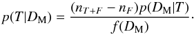 (2)Dividing both the numerator and the denominator by nT + F we recognize Bayes’ formula considering (nT + F−nF) /nT + F as the prior p(T) and considering either nF/nT + F as the prior p(F) or f(DM) = nT + Fp(DM).
The present paper basically extends this simple approach to more than two catalogues. Instead of fitting histograms to find the number of spurious associations, we directly compute them from the input catalogues data and from geometrical considerations.
Previously, Budavári & Szalay (2008) developed a multi-catalogue cross-match. For a given set of n sources from n distinct catalogues, they compute a “Bayes’ factor” based on both astrometric and photometric data. The “Bayes’ factor” is then used as a score: a pre-defined threshold on its value is applied to select or reject the given set of n sources. We discuss the astrometric part of Budavári & Szalay (2008) “Bayes’ factor” and compare it to our selection criterion in Sects. 5.6 and 6.1.
Throughout the present paper we consider a set of n catalogues. We use a Chi-square criterion based on individual elliptical positional errors to select, in these catalogues, sets of associations containing at most one source per catalogue. We call this selection a χ-match. We then compute probabilities for each set of associations. To compute probabilities, we consider only the result set in which each set of associations contains exactly n sources (one per catalogue, see below for partial matches). For people familiar with databases, it can be seen as the result of inner joins, joining successively each catalogue using a Chi-square criteria. The probabilities we then compute are only based on positional coincidences. Although we show how it is possible to add likelihoods based on photometric considerations, the computation of such photometric likelihoods is beyond the scope of this paper.
As the result of a χ-match, two distinct sets of associations may have sources in common: a source having a large positional error in one catalogue may for example be associated to several sources with smaller errors in another catalogue. We do not take into account in our probabilities the “one-to-several” and the “one-to-one” associations paradigms defined in Fioc (2014): it becomes far too complex when dealing with a generic number of catalogues and it is not that simple when a source may be blended, etc. We use a several-to-several-(to-several-...) paradigm. In other words, we compute probabilities for a set of associations regardless of the fact that a source in the set can be in other sets of associations. So a same detection in one catalogue may have very high probabilities of associations with several (sets of) candidates in the other catalogues. We think it is the responsibility of the photometric part to disentangle such cases.
Requiring one candidate per catalogue for each set of associations (i.e. each tuple) is somewhat restrictive. But, if one or several catalogues do not contain any candidates for a tuple, then we compute the probabilities from the cross-match of the subset of catalogues providing one candidate to that tuple. Those probabilities are computed independently of the “full” n catalogues probabilities. For example, if we cross-match three catalogues and if a set of associations (a tuple) contains one source per catalogues (A, B and C), then we will compute five probabilities: one for each possible configuration (ABC, AB_C, A_BC, AC_B and A_B_C in which the underscore “_” separates the catalogue entries associated to different actual sources, see Sect. 6.2.2). Now, if one source from A has a candidate in B and no candidate in C, we will compute only two probabilities (AB and A_B, see Sect. 6.2.1) considering only the result of the cross-match of A with B. Likewise for A and C only and for B and C only. These four cross-matches will yield eleven distinct probabilities. It is possible to deal with “missing” detections when computing photometrically based likelihoods (taking into account limit fluxes, ...) but it is not the case in the astrometric part of this work.
When χ-matching n catalogues, the number of hypotheses to be tested, and thus the number of probabilities to be computed for a given set of associations, increases dramatically with n. This number is 203 for 6 catalogues and reaches 877 for seven catalogues (see Table 2 in Sect. 6.2.4). To be able to compute probabilities when χ-matching more than seven catalogues we may start by merging catalogues for which the probability of making spurious associations is very low (e.g. catalogues of similar wavelength and similar astrometric accuracy), and handle the merged catalogue as a single input catalogue.
In Sect. 3 we lay down the assumptions we use to work on a simplified problem. We then (Sect. 4) define the notations and the standards used throughout the paper and link them to the standards adopted in a few catalogues. We then describe in detail the candidate selection criterion (Sect. 5) before providing (Sect. 6) an exhaustive list of all hypotheses we have to account for to apply Bayes’ formula. In Sect. 5 we also show how the “Bayesian cross-match” of Budavári & Szalay (2008) may be interpreted as an inhomogeneous χ-match. Then (Sect. 7) we show how it is possible to estimate the rates of spurious associations and hence “priors”. In Sect. 8 we compute an integral which is related to the probability the selection criterion has to select a set of n sources for a given hypothesis. This integral is crucial to compute likelihoods defined in Sect. 9 and to normalize likelihoods in Sect. 10. Finally, after showing how to introduce the photometric data into the probabilities (Sect. 11), and before concluding (Sect. 14), we explain the tests we carried out on synthetic catalogues in Sect. 12. Since this paper is long and technical, we put a summary of the steps to follow to perform a probabilistic χ-match in Sect. 13.
3. Simplifying assumptions
Cross-correlating catalogues taking into account an accurate model of the sky on one hand, and the effects and biases due to the catalogue building process on the other hand is a daunting task. To make progress towards this objective, we have to start by making simplifying assumptions.
First of all, we assume that there are no systematic offsets between the positions of each possible pair of catalogues. It means that the positions are accurate (no bias). We also assume that positional errors provided in catalogues are trustworthy. It means that they are neither overestimated nor underestimated: for instance, no systematic have to be quadratically added or removed. The first point supposes an accurate astrometric calibration of all catalogues. This is somewhat the “dog chasing its tail” problem since a proper astrometric calibration should be based on secure identifications, themselves based on... cross-identification! Ideally the astrometric calibration and the cross-identification should be performed simultaneously in an iterative process. It will not be developed here but we point out that the present work can be used to calibrate astrometrically n catalogues at the same time from one reference catalogue, taking into account all possible associations in all possible catalogue sub-sets. However, carrying out careful identification of primary or secondary astrometric standards is only important when the density of bright astrometric references is very low, typically in deep small field exposures. Reliable cross-identification is also crucial when the wavelength band of the image to calibrate differs widely from that of the astrometric reference image. In most large scale surveys such as 2MASS (Skrutskie et al. 2006) or SDSS (Pier et al. 2003) the density of bright Tycho-2 (Høg et al. 2000) or UCAC (Zacharias et al. 2004) astrometric reference stars is high enough to ensure an excellent overall calibration without any ambiguity in the associations.
Although the idealized vision of an immutable and static sky is long gone, we ignore proper motions in this analysis. There are at least two ways of taking them into account: either we may force associations to include at least one source from a catalogue containing measured proper motions; or we may try to fit proper motions during the cross-match process. In this last case, if a set of n sources detected at different epochs in n distinct catalogues does not satisfy the candidate selection defined in Sect. 5.2, we may make the hypothesis that they nonetheless are from a same source but having a proper motion. We can then estimate the proper motion and the associated error based on positions, (Gaussian) positional errors and epochs (see Appendix B). From the n observed positions and associated errors and from the n theoretical estimated positions and associated errors we can compute a Mahalanobis distance which follows a χ distribution with 2(n−2) degrees of freedom. Similarly to the candidate selection criterion in Sect. 5.2 we can then reject the hypothesis “same source with proper motion” if the Mahalanobis distance is larger than a given threshold.
We neglect clustering effects. We suppose that in a given area Ω, source properties are homogeneous. This implies that the local density of sources, the positional error distributions and the associations priors (probabilities of true associations that in principle depend on the astrophysical nature of the sources and on the limiting flux) are uniform over the sky area considered. As usual we have to face the following dilemma: on the one hand, the larger the area Ω, the better the statistic; on the other hand, the larger the area Ω, the less probable the uniform density, errors distributions and priors hypothesis. In the ARCHES project, for instance, we grouped the individual XMM-Newton EPIC fields of view of ≈0.126 deg2 each into installments of homogeneous exposure times and galactic latitude so as to ensure as much uniformity as possible. Each installment contained on the order of several hundred sources.
Finally, we neglect blending. If two sources are separated in one catalogue and blended in the other one, the position of the blended source will be something like the photocentre of the two sources. Either the blended source will not match any of the two distinct sources, or only one of the two distinct sources will match, the match likely being in the tail of the Rayleigh distribution, possibly leading to a low probability of identification. It will then not be problematic to consider the match as spurious since the observed flux is contaminated by the flux of the nearby source. Finally, if the positional accuracy of the blended source is well below that of the distinct sources, both distinct sources will match the blended source, leading to a non-unique association requiring further investigations to be disentangled.
4. Notations and links with catalogues
4.1. Notations
This article uses almost exclusively the notations defined in the ISO 80000-2:2009(E) international standard. Exceptionally we waive the notation detA for determinant and replace it by the equivalent but more compact notation | A |.
We consider n catalogues defined on a common surface of area Ω. We assume that each catalogue source has individual elliptical positional errors defined by a bivariate normal (or binormal) distribution. For this, we assimilate locally the surface of the sphere to its zenithal (or azimuthal) equidistant projection (see ARC projection in Calabretta & Greisen 2002), that is to its local Euclidean tangent plane. In this frame, the position of a point at distance d arcsec from the origin O (the tangent point) and having a position angle ϕ (east of north) is simply  This approximation is acceptable since typical positional errors, distances and surfaces locally considered are small.
We note  the binormal probability density function (p.d.f.) representing the position of a source S and its associated uncertainty:
 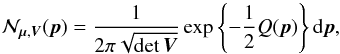 (5)with
-
μ = (μx,μy)⊺ the position of the source S provided in a catalogue, that is the mean of the binormal distribution;
-
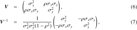
V the provided variance-covariance – also simply called covariance – matrix which defines the error on the source position;
-
p = (x,y)⊺ any given two-dimensional position;
-
Q(p) the quadratic form Q(p) = (p−μ)⊺V-1(p−μ), that is the square of the weighted distance between a given position p and the position of the source S
 where
where
-
σx is the standard deviation along the x-axis (i.e. the east axis);
-
σy is the standard deviation along the y-axis (i.e. the north axis);
-
ρ the correlation factor between σx and σy;
-
-
 the determinant of V;
 -
dp = dxdy.
A covariance matrix V represents a 1σ ellipse. The “real” position of the source S has ≈39% chances to be located inside this 1σ-ellipse. It must not be confused with the 1-dimensional 1σ-segment which contains a real “value” with a probability of ≈68%.
4.2. Classical positional errors in catalogues
In astronomical catalogues like the 2MASS All-Sky Catalog of Point Sources (2MASS-PSC, Cutri et al. 2003) positional errors are described by three parameters defining the 1σ positional uncertainty ellipse2: err_maj or a the semi-major axis, err_min or b the semi-minor axis, and err_ang or ψ the positional angle (east of north) of the semi-major axis. We give the formula to transform the ellipse into a covariance matrix (see Appendix A.2 of Pineau et al. 2011b and footnote 11 in Fioc 2014): 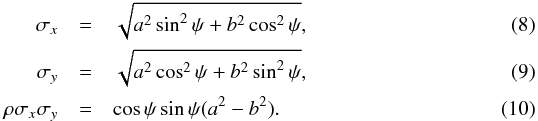 In the AllWISE catalogue (Cutri et al. 2014), the coefficients of the covariance matrix are (almost) directly available. Instead of providing the unitless correlation factor ρ or the covariance ρσxσy (in arcsec2), the authors chose to provide the co-sigma (σαδ) because, as they state3, the latter is in the same units as the other uncertainties. We thus have
  In catalogues like the Sloan Digital Sky Survey since its eighth data release (SDSS-DR8, Aihara et al. 2011) positional errors contain two terms: the error on RA (raErr) and the error on Dec (decErr). In this case the parameters of the covariance matrix are simply
 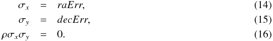 In catalogues like the XMM catalogues (e.g. the 3XMM-DR5, Rosen et al. 2016) a single error is provided. Ideally, one would like to have access to the two one-dimensional errors, even if their respective values are often very close. The column named radecErr is the total error, so the quadratic sum of the two computed (but not provided) 1-dimensional errors, one computed on RA and one computed on Dec. If one uses σx = radecErr and σy = radecErr, the total error will be
 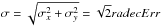 instead of radecErr. In output of the astrometric calibration process, the XMM pipeline provides a systematic error sysErrCC which is quadratically added to radecErr to compute the “total radial position uncertainty”4posErr. As for radecErr, we must divide posErr by
  to obtain the 1-dimensional error. The appropriate errors to be used (including a systematic) are then
 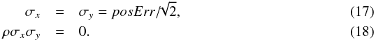 The factor has not been taken into account in Pineau et al. (2011b). It partly explains why the fit of the curve in the right panel of Fig. 3 mentioned in Sect. 5 of this paper does not lead to a Rayleigh scale parameter equal to 1.
Similarly to the XMM case, the error posErr provided in the GALEX All-Sky Survey Source Catalog (GASC) catalogue5 (which also includes the systematic) is a “total radial error”. It is thus the Rayleigh parameter σ which is the quadratic sum of two one-dimensional errors. As for XMM, the appropriate errors to be used are 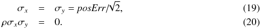 In catalogues like the ROSAT All-Sky Bright Source Catalogue (1RXS, Voges et al. 1999) the error provided is the radius of the cone containing the real position of a source with a probability of ≈68.269% (the 1 dimensional 1σ). Authors like Rutledge et al. (2003; given the details provided in Voges et al. 1999, Sect. 3.3.3) call this radius the 1σ-radius. We note it r68%. But, in the Rayleigh distribution, the scale parameter σ is defined such that the cone of radius r = σ contains the real position with a probability 100 × (1−exp(−1/2)) ≈ 39.347%. Adjusting such that
 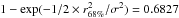 leads to
 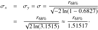 (21)Similarly if the provided error is the radius of the cone containing the real position with a probability of 90% (e.g. in the WGACAT, White et al. 2000)
  (22)The description (White et al. 1997) and the on-line documentation6 of the FIRST catalogue (Helfand et al. 2015a,b) provide an “empirical expression” to compute the semi-major and semi-minor axis of the 90% positional accuracy associated to each source:
 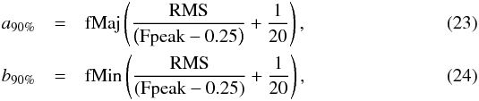 in which fMaj (fMin) is the major (minor) axis of the fitted FWHM, RMS “is a local noise estimate at the source position” and Fpeak is the peak flux density. The position angle ψ of the accuracy equals the fitted FWHM angle fPA. We first obtain the 1σ accuracy ellipse by resizing the 90% ellipse axes divinding them by the same factor as for the WGACAT (i.e.
  )
)  After possibly adding systematics, the variance-covariance matrix is obtained applying the equations used for the 2MASS catalogue.
Errors in catalogues like the Guide Star Catalog Version 2.3.27 (Lasker et al. 2007, GSC2.3) should not be used in the framework of this paper. As stated in Table 3 of Lasker et al. (2008): these astrometric and photometric errors are not formal statistical uncertainties but a raw and conservative estimate to be used for telescope operations.
Table 1 summarizes the transformation of catalogues positional errors into the coefficients of covariance matrices V.
Summary of the transformations of positional errors provided in various astronomical catalogues into the coefficients of error covariance matrices (before adding quadratically possible systematics).
5. Candidates selection: the χ-match
We make the hypothesis that n sources from n distinct catalogues are n independent detections of a same real source. With p the unknown position of the real source and μi the observed position of detection i, the probability for the n detections to be located at the observed positions is expressed by the joint density function: 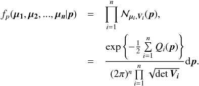 (27)
(27)
5.1. Estimation of the real position given n observations
We introduce the notations μΣ and VΣ for the weighted mean position of the n sources and its associated error respectively. The inverse of the covariance matrix VΣ is 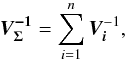 (28)leading to (see demonstration in Sect. A.1)
 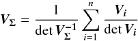 (29)which is used in the weighted mean position expression
 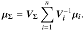 (30)Using both the weighted mean position and its error, the sum of quadratics in Eq. (27) can be divided into two parts and written as (see demonstration Sect. A.2)
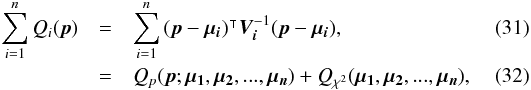 with
with 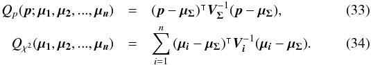 In the case of two catalogues the latter term can be written as in Eq. (51). Moreover, if both covariances are null, it takes the simple and common form
 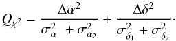 (35)Back to the general case, the term Qχ2 can also be put in the more computationally efficient form (only one loop over i)
 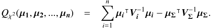 (36)From those formulae, it appears that the weighted mean position (Eq. (30)) is the maximum likelihood estimator of the “true” position of the source: the second term (Qχ2) is constant with respect to p so the maximum of the likelihood function ℒ(p;μ1,μ2,...,μn) = fp(μ1,μ2,...,μn | p) is obtained when the first term (Qp) is null, so when p = μΣ. The error on this estimate is simply VΣ, the inverse of the Hessian of the likelihood function.
5.2. Candidates selection criterion
For the candidate selection, we are interested in the probability the n sources have to be located at the same position. Let’s first rewrite Eq. (27) to exhibit a product of a binormal distribution by another multi-dimensional normal law: 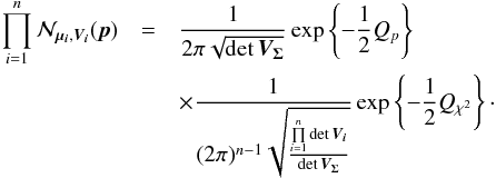 (37)When integrating Eq. (37) over all possible positions (i.e. over p) the first term integrates to 1, since it is the p.d.f. of a normal law in p, so we obtain
 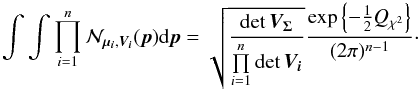 (38)We are supposed to integrate on the surface of the unit sphere. But the errors being small, we consider the infinity being at a relatively close distance, before effects of the sphere curvature become non-negligible.
In the previous equation, only the Qχ2 term remains. It can also be written (see demonstration Sect. A.3) 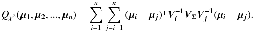 (39)Equation (38) is equivalent to P(D | H) in Budavári & Szalay (2008) and Eq. (39) – multiplied by the
  factor in the exponential (Eq. (38)) – is the generalization for elliptical errors of Eq. (B12) in Budavári & Szalay (2008). In practice, we never use Eq. (38) since the number of terms to be computed increases with O(n(n−1)/2) while it increases with O(n) in Eq. (36) or in its iterative form (see Eq. (48) in Sect. 5.3). We use here the big O notation, to be read as “the order of”.
We can see Eq. (34) as the result of a 2n-dimensional weighted least squares in which the model is the “real” position of the source and the solution is μΣ (by similarity with Eq. (31)). Putting all positional errors matrices in a 2n × 2n block diagonal matrix M, Qχ2 is the square of the Mahalanobis distance  defined by
 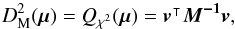 (40)
(40)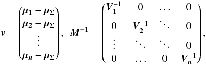 (41)which follows in our particular case a χ2 distribution with 2(n−1) degrees of freedom, or equivalently, (n−1)χ2 distributions with two degrees of freedom. Equation (40) is probably the Mahalanobis distance mentioned without giving its expression in Adorf et al. (2006).
If follows a  distribution, then its square root, the distance DM(μ), follows a χd.o.f. = 2(n−1) distribution.
We perform a statistical hypothesis test on a set of n sources, defining the null hyothesis H0 as follows: all sources in the set are detections of the same “real” source. The alternative hypothesis H1 would thus be: not all sources in the set are detections of the same “real” source; in other words the set of n sources contains at least one spurious source; or, expressed differently, the n sources are n observations of at least two distinct real sources. We adopt Fisher’s approach, that is we will reject the null hypothesis if, the null hypothesis being true, the observed data is significantly unlikely.
From now on, we indifferently write x or DM the Mahalanobis distance. Assuming the null hypothesis is true, the “theoretical” probability we had to get the actual computed (square of) Mahalanobis distance is given by a Chi(-square) distribution with 2(n−1) degrees of freedom: 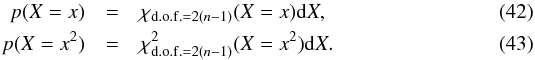 The probability we had to get an actual computed (square of) Mahalanobis distance less than or equal to a given threshold (or critical value)
  is given by the value of the cumulative distribution function of a the Chi(-square) at the given threshold
 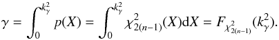 (44)We can indifferently work on x with the χ distribution or on x2 with the χ2 distribution. The threshold kγ we obtain on x is simply the square root of the threshold
  we obtain on x2. Although we find the Chi test more natural in the present case, most astronomers are familiar with the Chi-square test.
In the framework of statistical hypothesis tests, it is the complementary cumulative distribution (or tail distribution) function which is usually used by defining the p-value  (45)and a significance level α defined by
  (46)is fixed. The null hypothesis is then rejected if p - value <α. In the Neyman-Pearson framework α is the type I error, or the false positive rate, that is the probability the null hypothesis has to be rejected (positive rejection test) while it is true (wrong/false decision). In our case we fix γ (hereafter called completeness), the fraction of real associations we “theoretically” select over all real associations. The candidates selection criterion, or fail of rejection criterion, we use is then
  (47)in which
  or, equivalently,
  . This inequality is equivalent to p - value <α. It is important to write “fail of rejection” since nothing proves that if Eq. (47) is satisfied the null hypothesis is true: at this point the selected set of sources is nothing else than a set of candidates. Nevertheless we do call region of acceptance the set of DM(μ) values satisfying Eq. (47). This region of acceptance will be useful to define the domain of integration used to normalize likelihoods when computing probabilities for each hypothesis from Sect. 7. Its volume (see e.g. Eq. (64)) is the volume of the 2n-ellipsoid defined by M (see Eq. (40)) divided by the error ellipse associated to the weighted mean position μΣ and defined by VΣ (it thus is a volume in a 2(n−1) space).
In practice, the value is computed numerically using Newton’s method to solve  . The initial guess we use is the approximate value returned by Eq. (A.3) of Inglot (2010).
The value of γ we fix is independent of n, the number of candidates. In practice we often set this input parameter to γ = 0.9973. In one dimension this value leads to kγ = 3, that is the famous 3σ rule. It means that for 10 000 real associations in a dataset, we theoretically miss 27 of them by applying the candidate selection criterion. From now on we call this cross-correlation a χγ-match, or simply a χ-match.
In the particular case of two catalogues DM(μ) follows a χ distribution with 2 degrees of freedom – that is a Rayleigh distribution – and kγ = 0.9973 = 3.443935. This latter value is used in the two-catalogues χ-match of Pineau et al. (2011b).
5.3. Iterative form: catalogue by catalogue
Somewhat similarly to the Bayes factor in Budavári & Szalay (2008, Sect. 6) it is noteworthy that Qχ2 can be computed iteratively, summing (n−1) successive χ2 with two degrees of freedom computed from (n−1) successive two-catalogues cross-matches.
After each iteration, the new position to be used for the next cross-match is the weighted mean of all already matched positions and the new associated error is the error on this weighted mean. The strict equality between Eq. (48) and the non iterative form, for example Eq. (34), proves that the result is independent of the successive cross-matches order.
The maximum number of cross-matches to be performed must be known in advance in order to put an upper limit on kγ since it depends on the degree of freedom of the total χ2. The iteration formula is simply  (48)in which
 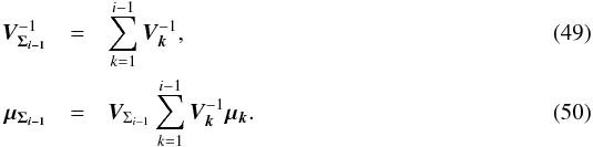 We find it from the 2-catalogues case, for which (see Sect. A.4)
  (51)We can demonstrate by direct calculation that
  (52)and so, iteratively, we find the general expression
 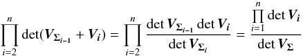 (53)which is consistent with Eq. (38). The volume of the acceptance region of the statistical hypothesis test is the volume of a 2(n−1) dimensional ellipsoid. More precisely, it is the product of the previous equation Eq. (53) by the volume of a 2(n−1)-sphere of radius kγ. This will be crucial when computing the rate of spurious associations.
5.4. Iterative form: by groups of catalogues
Instead of iterating over catalogues one by one, we can also perform G sub-cross-matches, each associating ng distinct sources such that  . We note Qχ2, { g } the square of the Mahalanobis distance associated with the group g:
 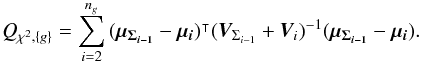 (54)We show that we can compute Qχ2 iteratively from the G weighted mean positions μΣ{g} and their associated errors
  . The square of the Mahalanobis distance can be written
 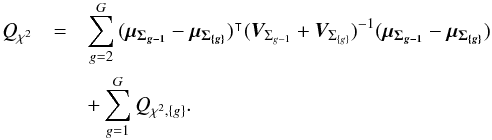 (55)In other words, the square of the Mahalanobis distance is the sum of the square of the intra-group Mahalanobis distances plus the inter-group iterative one. With k being an index defined inside each of the G groups { g }
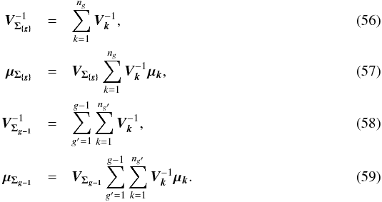 In fact, it is a straightforward generalization of the G = 2 groups case for which
 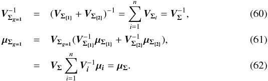 Here again,
 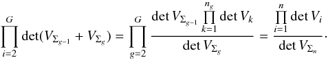 (63)Again, kγ depends on the number of degrees of freedom of the total χ2, thus on the total number of cross-correlated tables. It means that to be complete, all sub-cross-correlations must use the candidate selection threshold kγ(2(n−1)) computed from the total number of tables instead of kγ(2(ng−1)) computed from the number of tables in a group.
5.5. Summary and Interpretation
Equations (34), (36), (39), (40), (48) and (55) are all equivalent and they lead to the same value, that is to the same squared Mahalanobis distance. All sources are retained as possible candidates if Eq. (47) is verified, so if the Mahalanobis distance is smaller or equal to kγ. This threshold is the inverse of the cumulative χ distribution function at the chosen completeness γ, for 2(n−1) degrees of freedom.
As this criterion is no other than a χ-test criterion (or χ2-test criterion if we work on squared Mahalanobis distances) we call the result of such a criterion a χ-match.
The χ-match criterion defines a region of acceptance which is a 2(n−1)-ellipsoid of radius kγ. Its volume is computed from Eq. (53): ![Mathematical equation: \begin{equation} \mathcal{V}_n(k_\gamma) = \left[\frac{\prod\limits_{i=1}\det\bm{V_i}}{\det\bm{V_\Sigma}} \right]^{1/2} \frac{\pi^{n-1}k_\gamma^{2(n-1)}}{(n-1)!}, \label{eq:ellvolume} \end{equation}](/articles/aa/full_html/2017/01/aa29219-16/aa29219-16-eq187.png) (64)with
(64)with  the volume of a 2(n−1)-sphere of radius kγ. It will be later used to compute the expected number of spurious associations.
5.6. Comment on the “Bayesian cross-match” of Budavári & Szalay (2008)
We mention in Sect. 6.1 what appears to be a conceptual problem in calling B (Eq. (65)) a Bayes factor for more than two catalogues in the astrometrical part of Budavári & Szalay (2008).
Performing a cross-match by fixing a lower limit L on the “Bayes factor” B defined in Eq. (18) of Budavári & Szalay (2008) is no other than performing a χ-match with a significance level which depends both on the number of sources n and on the volume of the 2(n−1)-ellipsoid of radius 1. In fact, using the factor B of Budavári & Szalay (2008) in which wi is the inverse of the cirular error on the position of the source i and φij is the angular distance between sources i and j, we have the equivalence 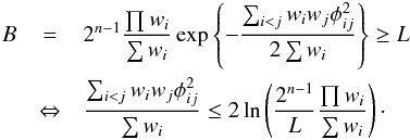 (65)We showed that the quantity on the left side of the inequality is equal to Eq. (39) in the present paper and thus follows a χ2 distribution for “real” associations. It means that the “Bayesian” candidate selection criterion B ≥ L is equivalent to a χ2 test having a significance level equal to
 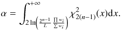 (66)The larger the volume of the 2(n−1)-ellipsoid of radius 1 (∝
 ), the more “real” associations are missed and the less spurious associations are retrieved. We could replace the criterion B ≥ L by
  . This is somewhere between the fixed radius cone search and the fixed significance level χ-match. The rate of missed “real” associations is not homogeneous but depends on the positional errors. Only if positional errors are constant in all catalogues, then the B ≥ L constraint becomes equal to the χ-match which is equal to a fixed radius cross-match.
6. Hypotheses from combinatorial considerations
A χ-match output is made of sets of associations, each set of associations containing one source per catalogue. For each set of associations we want to compute the probability all sources of the set have to come from a same actual source. In this section, especially in Sect. 6.2 we make explicit the sets { hi } of hypotheses we have to formulate to compute probabilities of identification when cross-correlating n catalogues.
6.1. Generalities
Given a set { hk } of pairwise disjoint hypotheses whose union is the entire set of possibilities, the law of total probabilities for an observable x is 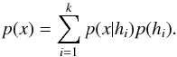 (67)Leading to Bayes’ theorem
 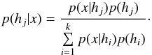 (68)We stress that Bayes’ factor (also called likelihood ratio) is defined only in cases involving two and only two hypotheses
 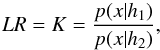 (69)and is used when no trustworthy priors p(h1) and p(h2) are available. We can transform any set of pairwise disjoint hypotheses into two disjoint hypotheses. In this case, using the negation notation ¬
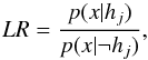 (70)with
 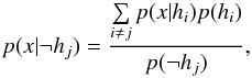 (71)and
  (72)Such a likelihood ratio (Eq. (70)) is not interesting since it is not only computed from likelihoods, but also from priors.
The term B(H | K) in Budavári & Szalay (2008, Eq. (8)) is improperly called Bayes factor when dealing with more than two catalogues. As a matter of fact, the union of the two hypotheses – all sources are from the same real source and each sources is from a distinct real source – is only a subset of all possibilities so the law of total probabilities and hence Bayes’ formula are not valid.
In Pineau et al. (2011b) the term LR(r) in Eq. (9) is also improperly called likelihood ratio since a likelihood is a probability density function and so integrates to 1 over its domain of definition. It is obviously not the case of dp(r | spur) in Eq. (8). The built quantity is related to the ratio between the probability the association has to be “real” over the probability it has to be spurious, but formally it is not a likelihood ratio. The very same “abuse of term” is made in Wolstencroft et al. (1986; who, moreover, adds a prior in the likelihood ratio), in Rutledge et al. (2000), Brusa et al. (2007) and probably other publications.
6.2. Possible combinations and the Bell number
Let’s suppose we have selected one set of n distinct sources from n different catalogues, one source per catalogue. Those n sources possibly are n detections of k distinct real sources, with k ∈ [1,n]. The case k = 1 corresponds to the situation where all sources are n observations of the same real source and the case k = n corresponds to the situation where there are n distinct real sources detected independently, one in each catalogue.
We call A the source from catalogue number one, B the source from catalogue number two and so on.
6.2.1. Two-catalogues case: two hypotheses
The classical two-catalogues case is trivial. We formulate only two hypotheses:
-
AB, the match is a real match, the two sources are two observations of a same real source, that is k = 1;
-
A_B, the match is spurious, the two sources are two observations of two different real sources, that is k = 2.
6.2.2. Three-catalogues case: five hypotheses
For three sources A, B and C from three different catalogues, we formulate five hypotheses:
-
ABC, all three sources come from a same real source, that is k = 1;
-
AB_C, A and B are from a same real source and C is from a different real source, that is k = 2;
-
AC_B, A and C are from a same real source and B is from a different real source, that is k = 2;
-
A_BC, B and C are from a same real source and A is from a different real source, that is k = 2;
-
A_B_C, all three sources are from three different real sources, that is k = 3.
6.2.3. Four-catalogues case: 15 hypotheses
For four sources A, B, C and D we have to formulate 15 hypotheses:
-
ABCD, when k = 1;
-
ABC_D, ABD_C, ACD_B and BCD_A, but also
-
AB_CD, AC_BD and AD_BC for k = 2;
-
AB_C_D, AC_B_D, AD_B_C, BC_A_D, BD_A_C and DC_A_B when k = 3;
-
A_B_C_D when k = 4.
6.2.4. n-catalogues case: Bell number of hypotheses
We now generalize to n catalogues. For each possible value of k, the number of ways the set of n sources can be partitioned into k non-empty subsets – each subset correspond to a real source – is given by the Stirling number of the second kind denoted  . The total number of hypotheses to be formulated is equal to the Bell number. The Bell number counts the number of partitions of a set and is given by
 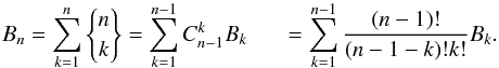 (73)Its seven first values are provided in Table 2 and a graphic illustration representing all possible partitions for five catalogues is provided in Fig. 18.
Values of the seven first Bell numbers.
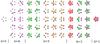 |
Fig. 1 The 52 partitions of a set with n = 5 elements. Each partition corresponds to one hypothesis for five distinct sources from five distinct catalogues. Left: k = 5, the five sources are from five distinct real sources. Right: k = 1, the five sources are from a same real source. (Tilman Piesk – CC BY 3.0 – modified – link in footnote). |
We face a combinatorial explosion of the number of hypotheses to be tested when increasing the number of catalogues. Although the theoretical developments presented here deal with any number of catalogues, the exhaustive analysis may be in practice limited to a few catalogues (n< 10).
Hereafter we note hi the hypothesis number i, we explicit it with letters for example hAB, and we note hk = i an hypothesis in which n observed sources are associated to i real sources.
7. Frequentist estimation of spurious associations rates and priors
We have defined a candidate selection criterion to perform χ-matches. We recall that we note x the Mahalanobis distance, and we note s the “event” x ≤ kγ, that is a given set of sources satisfies the selection criterion.
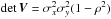
In a first step we want to estimate the number of “fully spurious” associations we would expect to find in a χ-match output and derive the prior p(hk = n | s) from this estimate. By “fully spurious” we mean that each candidate from each catalogue is actually associated with a different “real” source. A good such estimate is simply the mean sky area of the test acceptance region (see Eq. (64)) over all possible sources of all catalogues, multiplied by the number of sources in one of the catalogues and by the density of sources in the other ones. Written differently for n catalogues of ni sources each, on a common surface area Ω, it leads to an estimated number of spurious associations  equals to:
 ![Mathematical equation: \begin{equation} \hat{n}_{\Omega_{\rm spur}} = \frac{\pi^{n-1}k_\gamma^{2(n-1)}}{(n-1)!\Omega^{n-1}} \sum\limits_{i_1=1}^{n_1} \sum\limits_{i_2=1}^{n_2} ... \sum\limits_{i_n=1}^{n_n} \left[\frac{\prod\limits_{j=1}^n \det \bm{V_{i_j}}}{\det \bm{V_\Sigma}}\right]^{1/2}\cdot \label{eq:nfullyspur} \end{equation}](/articles/aa/full_html/2017/01/aa29219-16/aa29219-16-eq254.png) (74)Or, having histograms or more generally discretized positional error distributions:
(74)Or, having histograms or more generally discretized positional error distributions: ![Mathematical equation: \begin{equation} \hat{n}_{\Omega_{\rm spur}} = \frac{\pi^{n-1}k_\gamma^{2(n-1)}}{(n-1)!\Omega^{n-1}} \sum\limits_{b_1=1}^{N_1} \sum\limits_{b_2=1}^{N_2} ... \sum\limits_{b_n=1}^{N_n} \prod\limits_{k=1}^n c_{b_k}\left[\frac{\prod\limits_{j=1}^n \det \bm{V_{b_j}}}{\det \bm{V_\Sigma}}\right]^{1/2}, \label{eq:nfullyspurdisc} \end{equation}](/articles/aa/full_html/2017/01/aa29219-16/aa29219-16-eq255.png) (75)in which Nk are the numbers of bins in histograms – or number of points in a discrete distribution– and cbk are number of counts in given bins of a histogram. The number of counts may be replaced by the value of the discrete distribution (or weight wbk) times the number of elements: cbk = nkwbk.
(75)in which Nk are the numbers of bins in histograms – or number of points in a discrete distribution– and cbk are number of counts in given bins of a histogram. The number of counts may be replaced by the value of the discrete distribution (or weight wbk) times the number of elements: cbk = nkwbk.
To perform quick estimations using only a one dimensional error histogram per catalogue, we approximate elliptical errors by circular errors of same surface area.
The remainder of this section explains how we can compute priors from the rate of “fully spurious” associations and the number of associations found in all possible sub-cross-matches.
7.1. Case of two catalogues
Let’s suppose that we have two catalogues A and B and each catalogue contains only one source in the common surface area Ω. We note μa1, Va1 and μb1, Vb1 the position of the source and associated covariance matrix in A and B respectively. If we fix the position μa1 of the first source, the second source will be associated with the first one by a χγ-match if Eq. (47) is satisfied. So if the second source is located in an ellipse of surface area  centred around the position of the first source. We temporarily waive the ISO 80000-2 notation detM and replace it by the equivalent and more compact notation | M |. We also replace Va1 + Vb1 by V1,1 to rewrite the last term in the pithier form
  . We now suppose that both sources are unrelated and that μa1 and μb1 are uniformly distributed in Ω. Then, neglecting border effects, the probability that the two sources are associated by chance when performing a χγ-match is given by the ratio of the acceptance ellipse to the total surface area Ω:
  (76)We now suppose that the second catalogue contains nB sources uniformly distributed in Ω. And if all of them are unrelated to the source of the first catalogue, then the estimated number of spurious associations is simply the sum of the previous probability over the nB sources of the second catalogue
  (77)We now suppose that the first catalogue contains nA sources also uniformly distributed in Ω, all unrelated to catalogue B sources. Still neglecting border effects, the estimated number of spurious associations is simply the sum of the previous estimation over all catalogue A sources
  (78)In practice, evaluating this quantity can be time-consuming since we have to compute and sum nA × nB terms. Fortunately, we can evaluate it exactly for circular errors and approximately for elliptical errors computing only nA + nB terms. In fact
  in which
 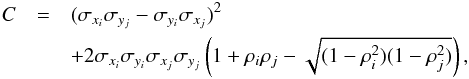 (83)and thus
 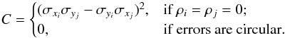 (84)For ordinary ellipses, that is ellipses having a position angle different from 0 and π/ 2, the approximation is valid if
  . In the particular case of circular errors, Eq. (78) becomes
 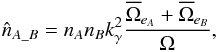 (85)in which
  and
and  are the mean surface area of all positional error ellipses in catalogues A and B respectively:
 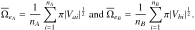 (86)For simple circular errors σai and σbi, this reduces to
 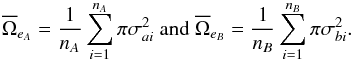 (87)If errors are constant for all sources in each catalogue, this reduces to
 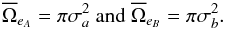 (88)These estimates based on geometrical considerations have the advantage of being very fast to compute.
Theoretically, we should remove from the double summation in Eq. (78) the pairs (i,j) which are real associations. We have no mean to do this since we do not known in advance the result of the cross-identification. Fortunately this effect is negligible in common cases. Indeed, if the result of the cross-match of the two catalogues contains nAB real associations – that is sources of both catalogues from a same real source – and supposing that the positional error distribution of sources having a counterpart is similar to the global error distribution we should modify Eq. (85) by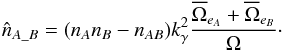 (89)In practice this estimate will tend to be overestimated since the distribution of sources in a catalogue cannot be uniform because of the limited angular resolution preventing the detection of very close sources in a same image. This effect is usually deemed to be of negligible importance. However one can detect its presence in particular circumstances. For instance, if the actual counterpart is located in the wings of a much brighter nearby source it may not be detected. This effect probably accounts for the presence of a fraction of the stellar identifications in high Galactic latitude X-ray surveys, in particular those with a much higher Fx/Fopt flux ratios and harder X-ray spectra than normal for active coronae in which cases a faint AGN may be the correct identification (Watson 2012; Menzel et al. 2016). One way to account for this effect and to limit the overestimation is to remove from the surface area Ω small areas around each source. The value of those areas depends for example on the source brightness. In addition, again because of the angular resolution: for real associations in catalogues having similar positional errors, the chance a source has to be also associated with a spurious source is low. More precisely, the start of the Poisson distribution will be truncated. In extreme cases in which the Poisson distribution is truncated for x<kγ, meaning that sources in a real association cannot be part of a spurious association, we should remove those sources from the estimate
  . We thus have to rewrite the previous equation Eq. (89) as
 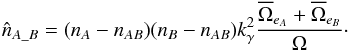 (90)Knowing the total number of associations, nT, resulting from the χ-match, we can estimate from Eq. (89) the number of spurious associations, and thus the number of real associations is estimated by
 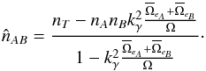 (91)If mean error ellipses in both catalogues are very small compared to the total surface area – that is
  – we can use the approximation
 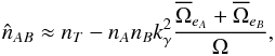 (92)which is equivalent to using directly equation Eq. (85), that is without taking care of removing real associations.
  is but an estimate and nothing prevents it from being negative due to count statistics in cross-matches with very few real associations and a lot of spurious associations. In practice, we have to define a lower limit such as
  .
.
Hence we can estimate the priors in the sample of associations satisfying the selection criterion (s) 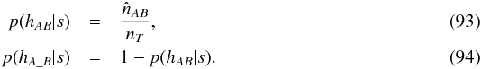 After a first two-catalogues cross-match, we may compare the expected histogram of detVi,j for spurious associations with the same histogram obtained from all associations. We may then derive the estimated distribution of this quantity (detVi,j) for “real” associations and compute the two likelihoods p(detVi,j | hAB,s) and p(detVi,j | hA_B,s).
Similarly we may build the histograms of the quantity detVΣ for both the spurious and the “real” associations. This quantity is the determinant of the covariance matrix – that is the positional error – associated with the weigthed mean positions. We proceeded likewise in Pineau et al. (2011b) using the “likelihood ratio” (see our comment on the abuse of term likelihood ratio) quantity instead of positional uncertainties.
7.2. Case of three catalogues
We recall that for 3 catalogues, the output contains five components (see Sect. 6.2.2): ABC, AB_C, A_BC, AC_B, A_B_C. We would like to estimate the number of spurious associations, that is the number of associations in the four components other than ABC. To do so, we need to perform the three two-catalogue cross-matches A with B, A with C and B with C. We are thus able to estimate nAB and nA_B, nAC and nA_C and finally nBC and nB_C respectively. To compute nAB_C, we proceed like in the previous section considering the two catalogues AB and C. AB is the result of the χ-match of A with B: the positions in catalogue AB are the weighted mean positions (μΣ, Eq. (30)) of associated A and B sources and the associated errors (or covariance matrix) are given by VΣ (Eq. (29)). The only difference with the two-catalogues case is that for the first catalogue (AB) we replace the simple mean elliptical error surface  over the nTAB entries by the weighted mean accounting for the probabilities the AB associations have to be “real” (i.e. not spurious)
 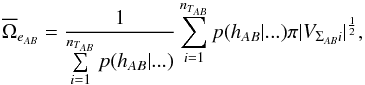 (95)in which p(hAB | ...) is the probability the association has to be a real association knowing some parameters (“...”), and VΣABi is the covariance matrix of the error on the weighted mean position i (see Sect. 5.3, particulary Eq. (49)). Such a probability will be computed in the next sections. We then compute
  and derive
  like in the two catalogues case replacing A by AB and B by C. Similarly to
, we can estimate
like in the two catalogues case replacing A by AB and B by C. Similarly to
, we can estimate  and
and  .
.
We now want to estimate nA_B_C, with a result which is independent from the cross-correlation order. Although we may use Eq. (74), it is possibly time consuming. Another solution is to use its discretized form Eq. (75). To do so quickly at the cost of an approximation we may circularize the errors by replacing the coefficients of the covariance matrix V by a single error equal to  and setting the correlation (or covariance) parameter equal to zero. It means that the new covariance matrix is diagonal and both diagonal elements are equal to . We choose this value to preserve the surface area of the two-dimensional error since the determinant (∝area) of the circular error equals the determinant (∝area) of the ellipse. This approximation is the same as the one made in the previous section. For each catalogue we then make the histogram of values using steps of for example one mas and we apply Eq. (75). In this case – circular errors – we simplify the equation using
 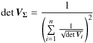 (96)and thus
 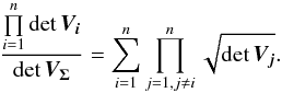 (97)We do not use this last form but give it for comparison with the denominator of Eq. (17) in Budavári & Szalay (2008).
Another option is to compute the number of “fully” spurious associations three times by following what was done in the previous section (and in the beginning of this section), but computing  instead of . Similarly to Eq. (95):
 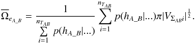 (98)Computing we derive
  . Similarly we can compute
  and
and  and estimate the number of fully spurious associations taking the mean of
,
and estimate the number of fully spurious associations taking the mean of
,  and
and  .
.
Having the estimated number of associations being part of the components AB_C, AC_B, A_BC and A_B_C plus knowing the total number of associations nT, we are able to estimate  and to compute the priors, for example
  (99)
(99)
7.3. Case of n catalogues
We can easily generalise the previous section using recursion. For n = 4 catalogues, we estimate the number of associations in component A_B_C_D knowing the number of associations in the result of the four-catalogue χ-match and estimating recursively (from the three-catalogue χ-matches) the number of associations in the 14 other components (AB_C_D, ...). So for n catalogues, the total number of distinct (sub)-cross-matches to be performed to compute all priors recursively is  (100)in which terms
  are the binomial coefficients (n−1) ! /(k ! (n−1−k) !). For five catalogues, Nχ−match = 26 and for six catalogues, Nχ−match = 57.
8. Probability of being χ-matched under hypothesis hi
In this section we compute p(s | hi), the probability that n sources from n distinct catalogues have to satisfy the candidate selection criteria under hypothesis hi. We will show in section Sect. 9 that the p.d.f. of the Mahalanobis distance for χ-match associations under hypothesis hi is the p.d.f. of the Mahalanobis distance without applying the candidate selection criteria, normalized by the probability p(s | hi) we compute in this section:  (101)We show here that p(s | hi) is proportional to the integral we note Ihi,n(kγ) (see Eq. (107)) which is independent of positional uncertainties and which also plays a role in Sect. 10. We will see also that p(s | hi) and Ihi,n(kγ) can be simplified to p(s | hk) and Ik,n(kγ) respectively, that is the probability n sources from n distinct catalogues have to satisfy the candidate selection criteria knowing they are actually associated with k distinct real sources.
If k = 1, that is all sources are from a same real source, we – logically – find p(s | hk = 1) = γ, the cumulative χ distribution function evaluated at the threshold kγ.
If k = n, all sources are spurious, we – also logically (see Eq. (74)) – find for Ik = n,n(kγ) the volume of a 2(n−1)-dimensional sphere of radius kγ, and p(s | hk = n) equals the volume of the 2(n−1)-dimensional ellipsoid defined by the test acceptance region divided by the common χ-match surface area raised to the power of the number of χ-matches (i.e. n−1).
We note x the total Mahalanobis distance, that is the square root of Eq. (36). The vectorial form x = (x1,x2,...xn−1) denotes the n−1 terms, also Mahalanobis distances, which are summed in the catalogue by catalogue iterative form Eq. (48). We rewrite this equation with the new notations  (102)So x is the radius of an hypersphere in the n−1 successive Mahalanobis distances space. The relation between x and x of dimension n−1 is the polar transformation F:Rn−1 → Rn−1, (x1,x2,...,xn−1) = F(x,θ1,...,θn−2),
 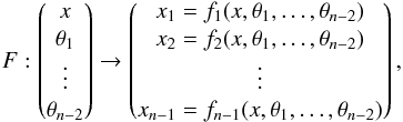 (103)with
 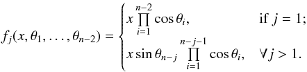 (104)The associated differential transform is
  (105)with JF the determinant of the Jacobian of F which is for example computed in Stuart & Ord (1994, Chap. II “Exact sampling distributions”, p. 375):
 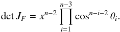 (106)We now define the Ik,n(kγ) integral which will be crucial in the next sections
 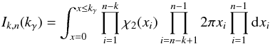 (107)in which k denotes the hypothetical number of real sources and so ranges from 1 to n. Written this way, the integral is simpler than the equivalent form:
 ![Mathematical equation: \begin{equation} I_{k,n}(k_\gamma) \!=\! \int_{x=0}^{x \le k_\gamma} \prod_{i=1}^{n_1-1} \rchi_2(x_i)\mathrm{d}x_i \left[ \prod_{g=2}^k\!\left( 2\pi x_{g-1}\mathrm{d}x_{g-1} \prod_{j=1}^{n_g-1} \rchi_2(x_j)\mathrm{d}x_j \right) \right] \label{eq:ikndef2} \end{equation}](/articles/aa/full_html/2017/01/aa29219-16/aa29219-16-eq365.png) (108)in which we have k groups containing each ng sources associated to a same real source so that
(108)in which we have k groups containing each ng sources associated to a same real source so that  (see the iterative candidate selection by groups of catalogues in Sect. 5.4). Here Eq. (55) takes the form
 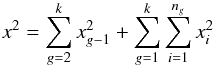 (109)where xg−1 are inter-group Mahalanobis distances and xi are intra-group Mahalanobis distances. In this version of the formula, we suppose that we iteratively cross-correlate the catalogues by groups. We suppose that each group corresponds to one real source. So inside each group, we multiply Rayleigh distributions and when associating each group, we multiply by two-dimensional Poisson distributions.
We compute Ik,n using recursive integration by parts, leading to (see Sects. A.5.3 and A.6) 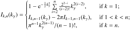 (110)We provide the exhaustive list of values of Ik,n(kγ) for n = 2,3,4 and 5 in Table 3. Remark: kγ depends on the selected completeness γ and on the number of catalogues n. When we call Ik,n−k(kγ), the kγ to be used in the integral is always the kγ computed for n catalogues. So I1,n−k will no longer be equal to γ but to Fχ2(n−k−1)(kγ). For example, we fix γ to 0.9973. Then for a n = 2 catalogues χ-match, kγ ≈ 3.4 and I1,2 = γ. But for a n = 3 catalogues χ-match, kγ ≈ 4.0, I1,3 = γ and I1,3−1 = 2 ≠ γ.
Values of the normalization integrals Ik,n−k(kγ) for a number of catalogue ranging from two to five.
Values of the derivatives of normalization integrals for a number of catalogue ranging from two to five.
We call p(s | hk) the marginalized probability of observing a Mahalanobis distance less than or equal to kγ in a group of n sources knowing they are actually associated to k real sources. ![Mathematical equation: \begin{equation} p(s|h_k) = \begin{cases} I_{k,n}(k_\gamma), & \text{ if } k=1; \\ \left[\frac{\prod\limits_{i=1}^n \det \bm{V_i}}{\det \bm{V_\Sigma}}\right]^{1/2} \frac{1}{\Omega^{(k-1)}}I_{k,n}(k_\gamma), & \text{ if } k > 1. \end{cases} \label{eq:pshk} \end{equation}](/articles/aa/full_html/2017/01/aa29219-16/aa29219-16-eq414.png) (111)We obtain this equality by replacing 2πxg−1 by 2πxg−1det(VΣg−1 + VΣg)/Ω in Eq. (108) and then applying Eq. (63). The factor 1/Ω comes from the normalisation of the Poisson distribution so it integrates to one over the common surface area of the cross-matched catalogues. For the particular case in which all sources are spurious, we logically find the summed terms in Eq. (74).
(111)We obtain this equality by replacing 2πxg−1 by 2πxg−1det(VΣg−1 + VΣg)/Ω in Eq. (108) and then applying Eq. (63). The factor 1/Ω comes from the normalisation of the Poisson distribution so it integrates to one over the common surface area of the cross-matched catalogues. For the particular case in which all sources are spurious, we logically find the summed terms in Eq. (74).
And the distribution (p.d.f.) associated to the probability p(x | hk) of observing a given Mahalanobis distance x knowing hk is simply given by the derivative of p(s | hk)dx, so is proportional to dIk,n(x)dx.
9. Simple Bayesian probabilities
In this section, we compute Bayesian probabilities which depend on the Mahalanobis distance only.
9.1. General formula
Given a set of n candidates from n distinct catalogues satisfying the candidate selection criterion, we know
-
x, the Mahalanobis distance (Eq. (40)), or χ value, which is a real value;
-
s, the result of the selection criterion x ≤ kγ, that is a boolean always equals to true for the sets of associations we keep, so p(s) = 1;
-
{ hi }, i ∈ [1,Bn], the set of Bn (Eq. (73)) hypotheses to be formulated for each set of association.
We then note hk hypotheses in which the n sources are associated with k “real” sources.
For a given set of n candidates from n distinct catalogues, the probabilities associated with the various hypotheses are given by Bayes’ formula  In this formula, p(hi | s) are priors (considering only χ-matches, hence only s = true) and correspond to the number of associations satisfying the candidate selection (χ-matches) and hypotheses hi over the total number of associations satisfying the candidate selection. We can transform the likelihood p(x | hi,s) in
  because we keep in our sample only associations satisfying the candidate selection criteria we have p(s | x,hi) = 1. In other words, the likelihood we use is a classical likelihood normalized so it integrates to one over the χ test acceptance region (defined by x ≤ kγ).
We easily compute priors from the numbers estimated in Sect. 7. And likelihoods are simply computed from Sect. 8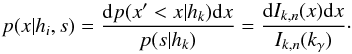 (117)We make explicit this result in the next section for the case of two, three and four catalogues.
9.2. Likelihoods p(x|hi,s)
In this section, we compute the likelihoods p(x | hi,s), that is the p.d.f. of the Mahalanobis distance of χ-matches under hypothesis hi.
9.2.1. Case of two catalogues
For a set of two sources from two distinct catalogues, we have only two hypotheses, hence the two likelihoods: 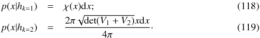 Knowing that the selection criterion is satisfied, we have to normalize so the integral of each likelihood over the domain defined by the selection criteria equals one (likelihoods are p.d.f.):
  All constant terms, that is terms independent of x, vanish with the normalisation. The likelihoods are plotted in Fig. 2.
Remark: p(x | hk = 2) mixes the derivative of the surface area of an ellipse in the Euclidean plane and the surface area of the sphere. It is an approximation valid as long as  is small enough so effects of the curvature of the sphere are negligible.
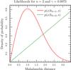 |
Fig. 2 Two possible likelihoods for n = 2 catalogues and γ = 0.9973: normalized Rayleigh (red, filled curve) and Poisson (green, dashed curve) components. We note that this γ value implies the [0,kγ = 3.443935] range for x. |
9.2.2. Case of three catalogues
For a set of three sources A, B, and C from three distinct catalogues, we have five hypotheses (see Sect. 6.2.2). In the five hypotheses, the number of “real” sources can be either one, two or three. We have as many likelihoods as possible distinct number of “real” sources. There are three ways of performing an iterative cross-match, leading to the same Mahalanobis distance x:
-
cross-match A with B and then with C,
 ;
; -
cross-match B with C and then with A,
 ;
; -
cross-match A with C and then with B,
 .
.
We denote xAB the Mahalanobis distance between A and B and we denote xABC the Mahalanobis distance between C and the weighted mean position of A and B.
x1 and x2 are used to designate without distinction xAB, xBC or xAC and xABC, xBCA or xACB respectively.
Although it may be tempting to write ![Mathematical equation: \begin{eqnarray} p(x_{AB}, x_{ABC}|h_{ABC}) & = & \frac{\rchi(x_{AB})\rchi(x_{ABC})\mathrm{d}x_{AB}\mathrm{d}x_{ABC}} {I_{1,3}(k_\gamma)}, \\[2mm] p(x_{AB}, x_{ABC}|h_{AB\_C}) & = & \frac{\rchi(x_{AB})2\pi x_{ABC}\mathrm{d}x_{AB}\mathrm{d}x_{ABC}} {I_{2,3}(k_\gamma)}, \\[2mm] p(x_{AC}, x_{ACB}|h_{AC\_B}) & = & \frac{\rchi(x_{AC})2\pi x_{ACB}\mathrm{d}x_{AC}\mathrm{d}x_{ACB}} {I_{2,3}(k_\gamma)}, \\[2mm] p(x_{BC}, x_{BC\_A}|h_{A\_BC}) & = & \frac{\rchi(x_{BC})2\pi x_{BC\_A}\mathrm{d}x_{BC}\mathrm{d}x_{BCA}} {I_{2,3}(k_\gamma)}, \\[2mm] p(x_{AB}, x_{ABC}|h_{A\_B\_C}) & = & \frac{2\pi x_{AB} 2\pi x_{ABC}\mathrm{d}x_{AB}\mathrm{d}x_{ABC}} {I_{3,3}(k_\gamma)}, \end{eqnarray}](/articles/aa/full_html/2017/01/aa29219-16/aa29219-16-eq450.png) we cannot directly compute probabilities p(hi | x) from those likelihoods since infinitesimals (dxAB, dxAC, ...) are not the same and so do not vanish when applying Bayes’ formula.
we cannot directly compute probabilities p(hi | x) from those likelihoods since infinitesimals (dxAB, dxAC, ...) are not the same and so do not vanish when applying Bayes’ formula.
It seems that the only measurement one can use to obtain coherent (and symmetrical) probabilities is the total Mahalanobis distance x. So we have to integrate the above probabilities over the domain defined by  and then evaluate their derivatives for x. We obtain the following likelihoods represented in Fig. 3.
 ![Mathematical equation: \begin{eqnarray} p(x|h_{k=1},s) & = & \frac{\mathrm{d}I_{1,3}(x)\mathrm{d}x}{I_{1,3}(x)} = \frac{\rchi_{{\rm d.o.f.}=4}(x)\mathrm{d}x}{\gamma}, \\[2mm] p(x|h_{k=2},s) & = & \frac{\mathrm{d}I_{2,3}(x)\mathrm{d}x}{I_{2,3}(x)} = \frac{2x(1-\exp(-x^2/2))\mathrm{x}}{k_\gamma^2-2(1-\exp(-k_\gamma^2/2))},\\[2mm] p(x|h_{k=3},s) & = & \frac{\mathrm{d}I_{3,3}(x)\mathrm{d}x}{I_{3,3}(x)} = \frac{4x^3\mathrm{x}}{k_\gamma^4}, \end{eqnarray}](/articles/aa/full_html/2017/01/aa29219-16/aa29219-16-eq455.png) in which hk = 1 is the hypothesis hABC, hk = 3 is the hypothesis hA_B_C and hk = 2 is either the hypothesis hAB_C or hAC_B or hA_BC.
in which hk = 1 is the hypothesis hABC, hk = 3 is the hypothesis hA_B_C and hk = 2 is either the hypothesis hAB_C or hAC_B or hA_BC.
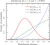 |
Fig. 3 Three possible likelihoods p(x | hk,s) for n = 3 catalogues and γ = 0.9973: χ distribution with four degrees of freedom (red, filled curve); Integral of a χ distribution with two degrees of freedom times a two-dimensional Poisson distribution (green, dashed curve); Four-dimensional Poisson distribution (blue, dotted curve). |
9.2.3. Case of four catalogues
For a set of four sources A, B, C and D from four distinct catalogues, we have fifteen hypotheses (see Sect. 6.2.3). In the fifteen hypotheses, the number of “real” sources can be either one, two, three or four. We have as many likelihoods as possible distinct numbers of “real” sources. They are represented in Fig. 4: ![Mathematical equation: \begin{eqnarray} p(x|h_{k=1},s) & = & \frac{\mathrm{d}I_{1,4}(x)\mathrm{d}x}{I_{1,4}(x)} = \frac{\rchi_{{\rm d.o.f.}=6}(x)\mathrm{d}x}{\gamma}; \\ p(x|h_{k=2},s) & = & \frac{\mathrm{d}I_{2,4}(x)\mathrm{d}x}{I_{2,4}(x)}; \\[2mm] p(x|h_{k=3},s) & = & \frac{\mathrm{d}I_{3,4}(x)\mathrm{d}x}{I_{3,4}(x)}; \\[2mm] p(x|h_{k=4},s) & = & \frac{\mathrm{d}I_{4,4}(x)\mathrm{d}x}{I_{4,4}(x)} = \frac{6x^5\mathrm{d}x}{k_\gamma^6}\cdot \end{eqnarray}](/articles/aa/full_html/2017/01/aa29219-16/aa29219-16-eq465.png) In which hk = 1 is the hypothesis hABCD; hk = 4 is the hypothesis hA_B_C_D; hk = 2 is either the hypothesis hA_BCD or hB_ACD or hC_ABD or hD_ABC or hAB_CD or hAC_BD or hAD_BC; and hk = 3 is either the hypothesis hAB_C_D or hAC_B_D or hAD_B_C or hBC_A_D or hBD_A_C or hCD_A_B.
In which hk = 1 is the hypothesis hABCD; hk = 4 is the hypothesis hA_B_C_D; hk = 2 is either the hypothesis hA_BCD or hB_ACD or hC_ABD or hD_ABC or hAB_CD or hAC_BD or hAD_BC; and hk = 3 is either the hypothesis hAB_C_D or hAC_B_D or hAD_B_C or hBC_A_D or hBD_A_C or hCD_A_B.
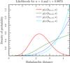 |
Fig. 4 Four possible likelihoods p(x | hk,s) for n = 4 catalogues and γ = 0.9973: χ distribution with six degrees of freedom (red, filled curve); integral of a χ distribution with two degrees of freedom times a four-dimensional Poisson distribution (green, dashed curve); integral of a χ distribution with four degrees of freedom times a two-dimensional Poisson distribution (blue, dotted curve); six-dimensional Poisson distribution (cyan, filled curve). |
9.3. Advantage and limits
The main advantage of using p(hi | x,s) is that the likelihoods it is based on do not depend on the positional errors: the only input parameter is the Mahalanobis distance x. Although it is true that x is computed from positional errors, once the χ-match has been performed we do not need the errors anymore: the distributions we use relies only on x. Changing positional errors modifies the priors, not the likelihoods. So we can easily add independent likelihoods based on magnitudes or other parameters.
There are two main problems. The first problem is precisely that the likelihoods depend only on x. It means that a set of very close sources with very accurate positions may have the same probability than a set of distant sources with large positional errors, even if intuitively the risk the first set have to contain spurious association should be far lower than in the second case. The second limitation is due to the fact that likelihoods are the same for hypotheses considering the same number of “real” sources. In the three catalogues case, p(x | hAB_C,s) = p(x | hA_BC,s) = p(x | hAC_B,s). The priors being constants, if p(hAB_C | s) >p(hA_BC | s) >p(hAC_B | s), we always obtain posterior probability p(x | hAB_C,s) >p(hA_BC | s) >p(hAC_B | s).
10. Bayesian probabilities with positional errors
In this section, we compute Bayesian probabilities which include explicitly positional errors.
10.1. Warning about the non independence of positional uncertainties
In surveys providing individual uncertainties, positions of unsaturated bright sources are often more precise than positions of faint sources. The reason has to do with the higher photometric signal-to-noise ratio of bright sources compared to faint sources, while the FWHM is similar. An example of computation of positional uncertainties based on photon statistics can be found for example in the documentation of the SExtractor software (Bertin & Arnouts 1996). As mentioned in the documentation, the photon statistics based error is a lower value estimate.
It means that we cannot blindly assume that the positional uncertainties and photometric quantities like apparent magnitudes are independent. Moreover, if the positional errors of sources are related to their magnitudes and if the magnitudes of the sources in different catalogues are also related, then positional uncertainties in the different catalogues are related too. It means that we cannot blindly assume that the positional uncertainties of matching objects in different catalogues are independent from each other, at least not for hk<n, that is the hypothesis in which at least two sources are from a same actual source.
One has to keep this in mind when using the naive independent hypothesis to simplify Bayes probabilities.
10.2. Probability using the Mahalanobis distance
To (at least partly) solve the first issue mentioned in Sect. 9.3 one possibility is to introduce likelihoods based for example on the volume V of the Chi test acceptance region writing: 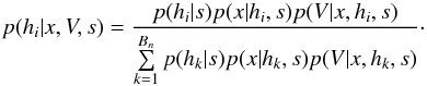 (134)From Sect. 7, it is easy – even though it may be time consuming – to build the estimated histogram nA_Bp(V + ΔV | hA_B) (in which ΔV is the width of the histogram’s bars). Given this histogram and the result of a two-catalogues cross-match, we can also build an estimated histogram nABp(V + ΔV | hAB). And so on for multiple catalogues, performing all possible sub-cross-matches.
If V and x are independent for all hypotheses, and knowing (having estimates of) nAB and nA_B, we have all the ingredients to compute 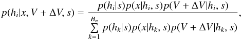 (135)even if it is not elegant to introduce a somewhat arbitrary slicing in V histograms.
10.3. Putting aside the Mahalanobis distance
We also consider the alternative form which puts aside the Mahalanobis distance and relies on the full sets of positions μ and associated errors V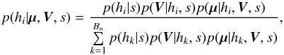 (136)in which the probabilities explicitly depend on the “configuration” of each position and on the associated errors. It also depends on the distribution of positional errors for a given hypothesis. Although p(V | hi,s) can be estimated performing all possible sub-cross-matches, it is not trivial since it is a joint distribution in a space of dimension equal to the number of “actual” sources considered in hi (using the circular error approximation).
10.3.1. Likelihoods p(μ |hi, V, s)
We make the hypothesis that ng sources are ng detections of a same true source having a given position p. The probability to observe the set of positions μ{g} = { μ1,μ2,...,μng }, knowing p and the set of errors V{g} = { V1,V2,...,Vng } is 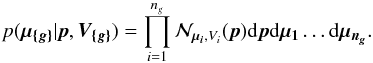 (137)In practice we do not know the position of the real source p. So the probability to observe the set of positions μ{g} knowing the set of errors V{g} is obtained by integrating over all possible positions
 ![Mathematical equation: \begin{eqnarray} p( \vec{\mu_{\{g\}}} | \bm{V_{\{g\}}} ) & = & \left( \int\int \prod\limits_{i=1}^{n_g}\mathcal{N}_{\vec{\mu_i},V_i}(\vec{p}) \mathrm{d}\vec{p} \right) \mathrm{d}\vec{\mu_1}\dots\mathrm{d}\vec{\mu_{n_g}}, \\[2mm] & = & \sqrt{ \frac{\det \bm{V_{\Sigma_{\{g\}}}}} {\prod\limits_{i=1}^{n_g}\det\bm{V_i} }} \frac{\exp\left\{-\frac{1}{2} Q_{\rchi^2(\vec{\mu_1},\vec{\mu_2},...,\vec{\mu_{n_g}})}\right\}} {(2\pi)^{n_g-1}} \nonumber\\[2mm] & & \times \mathrm{d}\vec{\mu_1}\dots\mathrm{d}\vec{\mu_{n_g}}. \end{eqnarray}](/articles/aa/full_html/2017/01/aa29219-16/aa29219-16-eq503.png) This result is the same as Eq. (38) in Sect. 5.2 but applied here to the sub-set of positions { μ1,μ2,...,μng }. The difference is that in Sect. 5.2 we wanted to estimate the probability the sources had to be at the same location whereas here, knowing (making the hypothesis) they are at the same location, we compute the probability we had to observe this particular outcome. The particular case ng = 1 leads to p(μ{g} | V{g}) = dμ1.
This result is the same as Eq. (38) in Sect. 5.2 but applied here to the sub-set of positions { μ1,μ2,...,μng }. The difference is that in Sect. 5.2 we wanted to estimate the probability the sources had to be at the same location whereas here, knowing (making the hypothesis) they are at the same location, we compute the probability we had to observe this particular outcome. The particular case ng = 1 leads to p(μ{g} | V{g}) = dμ1.
We now consider G groups and the selection criteria s (x ≤ hγ). Each of the n input sources is part of one, and only one group. Given the G groups, the errors on the positions and the candidate selection criteria, the probability to observe positions μ is 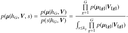 (140)The denominator ensures that the likelihood integrates to one over its domain of definition, domain delimited by the candidate selection criteria, that is the region of acceptance of the χ2 test.
Let us compute the integral in the denominator. The differential of the substitution x = yV-1y transforms as  . y can be the difference between two positions (e.g. μi−μΣi−1) and (x,θ) the polar coordinates of y in the basis defined by the eigenvectors of V and reduced by its eigenvalues. V can for example be VΣi−1 + Vi. Using the iterative form of Sect. 5.3 and Eq. (53), we can rewrite p(μ{g} | V{g})
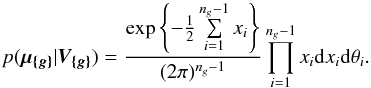 (141)Integrating over all θi we obtain
 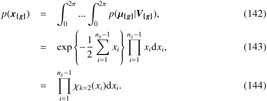 This joint p.d.f. of the successive Mahalanobis distances is different from the p.d.f. of their quadratic sum which gives the total Mahalanobis distance
  (145)in which
  .
.
Putting all together, the integral in the denominator is no other than the integral Ik = G,n(kγ) defined in Sect. 8. Written explicitly: 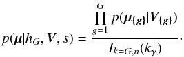 (146)
(146)
10.3.2. Classical two catalogues case
In the case of two catalogues, the probabilities are simply:
![Mathematical equation: \begin{eqnarray} && p(\vec{\mu_1}, \vec{\mu_2}|h_1,\bm{V_1},\bm{V_2},s) = \frac{\exp\left\{-\frac{1}{2} x^2\right\} \mathrm{d}\vec{\mu_1}\mathrm{d}\vec{\mu_2}} {2\pi\sqrt{\det(\bm{V_1} + \bm{V_2})} \gamma};\\[2mm] && p(\vec{\mu_1}, \vec{\mu_2}|h_2,\bm{V_1},\bm{V_2},s) = \frac{\mathrm{d}\vec{\mu_1}\mathrm{d}\vec{\mu_2} } {\pi k_\gamma^2 }\cdot \end{eqnarray}](/articles/aa/full_html/2017/01/aa29219-16/aa29219-16-eq523.png)
If we compare the likelihood ratio LRμ,V computed from those formulae with the likelihood ratio LRx computed from the previous result (Sect. 9.2.1) we obtain: ![Mathematical equation: \begin{eqnarray} LR_x & = & \frac{k_\gamma^2 {\rm e}^{-x^2/2}}{2\gamma}; \\[2mm] LR_{\vec{\mu},\bm{V}} & = & \frac{k_\gamma^2 {\rm e}^{-x^2/2}}{2\gamma\sqrt{\det(\bm{V}_1 + \bm{V}_2)}}\cdot \end{eqnarray}](/articles/aa/full_html/2017/01/aa29219-16/aa29219-16-eq526.png) Contrary to LRx, LRμ,V accounts for the size of positional errors. As we will see in the next section, the drawback is that we can hardly combine the likelihoods p(μ1,μ2 | hk,V1,V2,s) with photometry based likelihoods.
Contrary to LRx, LRμ,V accounts for the size of positional errors. As we will see in the next section, the drawback is that we can hardly combine the likelihoods p(μ1,μ2 | hk,V1,V2,s) with photometry based likelihoods.
11. Bayesian probabilities with photometric data
All probabilities of association discussed so far are based on the likelihood that the positions recorded in various catalogues are consistent with that of a unique astrophysical object. However, one may wish to make additional assumptions on the nature of the source (e.g. star, active galactic nucleus, etc.) that could help decrease or, conversely, increase the plausibility of a given association of catalogue entries. This is particularly important when one seeks to gather homogeneous samples of objects. Spectral energy distributions assembled from photometric catalogues can be usefully compared with templates and assigned a probability of being representative of the targeted class of objects. This procedure has been presented in Budavári & Szalay (2008) and recently used in Naylor et al. (2013) and Hsu et al. (2014). However, following Budavári & Szalay (2008) we underline that entering criteria of resemblance to a given class of objects in the computation of association probabilities is done at the expense of the capability to find scientifically interesting outliers.
Another possibility may consist in building colour-colour diagrams for random and χ-matched associations to derive colour-colour diagrams for real associations (more precisely, we have to derive each diagram for each possible hypothesis hi). Those normalized diagrams are p.d.f. that can be interpreted as likelihoods (p(m | hi,s) in the following equations). Smoothing those diagrams, one can see them as the likelihoods of the kernel density classification (Richards et al. 2004), replacing the object types by the hypothesis hi, and using magnitudes from different catalogues instead of just one.
We detail below how photometric data can be folded into the output of the purely astrometric method discussed in this paper, without making additional assumptions on the nature of the source.
Suppose we note a, a vector containing all the astrometric information we have about a set of n candidates (a may contain the positions, the associated covariance matrices, ...). We note m the set of photometric informations we have about the same set of n candidates (m may contain magnitudes and/or colours, associated errors, ...). Then we can write the Bayes formula: 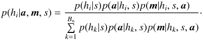 (151)If a and m are independent (naive hypothesis which is not granted, see Sect. 10.1)
 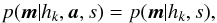 (152)and Eq. (151) becomes
 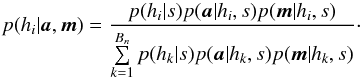 (153)Let’s imagine we perform a cross-match taking into account astrometric data only. We compute probabilities p(hi | a,s) for all possible hypotheses. Then if a and m are independent, and if we are able to compute likelihoods based on photometric data only p(m | hi,s), then we can compute the probabilities p(hi | a,m,s) in a second step from the probabilities computed in the astrometric part:
  (154)which is equivalent to Eq. (153).
Unfortunately, positional errors and magnitudes are not necessarily independent. So one should not use p(hi | μ,V,s) without any due caution in Eq. (154). However, one can use the Mahalanobis distance x which is independent of the photometry, that is probabilities p(hi | x,s) (Eq. (113)).
12. Tests on synthetic catalogues
In the context of the ARCHES project, we developed a tool implementing the statistical multi-catalogue cross-match described in this paper. We added to the tool the possibility to generate synthetic catalogues that can be cross-matched like real tables. It has been allowing us to perform tests and to check both the software and the theory.
We present here such a test and provide the associated script (see Appendix C) so anybody can try it independently, possibly changing the input values. Currently the tool is accessible both via a web interface and an HTTP API9. Future plans are discussed in the conclusion Sect. 14.
We generate three synthetic catalogues, setting the numbers of sources they contain and have in common: we call nABC the number of common sources in the three catalogues A, B and C; nAB the number of common sources in A and B only; nA the number of sources in catalogue A only; and so on. Knowing a priori common and distinct sources in the catalogues, we can track the associations which are real and the spurious ones in the cross-match output. We can also check for missing associations.
The error associated to each individual position is a random value which follows a user define distribution. A different distribution is used for each catalogue. For catalogue A, we choose a constant value equal to 0.4′′; for catalogue B, the positional error distribution follows a linear function between 0.8′′ and 1.2′′; for catalogue C, the positional errors follow a Gaussian distribution of mean 0.75′′ and standard deviation 0.1′′ truncated to the 0.5–1′′ range.
We set the input sky area to be a cone of radius 0.42 degrees. Each position is randomly (uniform distribution) placed in this cone. For each catalogue in which the source is included, we randomly pick a positional error that we associate to the source and we blur the position using its error.
We first compute  for pairs AB, AC and BC. Given the chosen error distributions, the mean errors are equal to the median errors and the mean of the inverse of the errors is quite close to the inverse of the mean errors. So, for this particular case, we use the inverse of the mean errors 0.4, 1 and 0.75 instead of the means of the inverse. Given this approximation and using Eq. (96), we obtain
 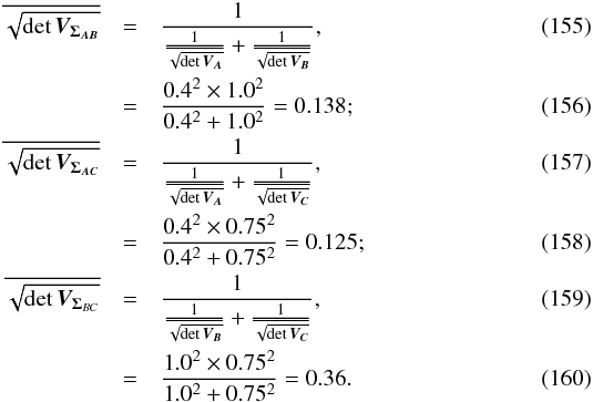 And, to estimate the number of “fully” spurious associations, we have to compute the mean of the square root of Eq. (97) over all possible source trios, which can be approximated in this specific case by
 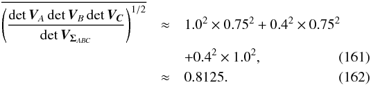 We note that in this particular case, the error distribution of sources A involved in AB, AC and ABC associations is the same. Idem for the error distribution of B and C sources.
We are now able to compute all components, depending on the size of histograms bins (step). To do this we note ![Mathematical equation: \begin{eqnarray} n_{AB*} & = & n_{ABC} + n_{AB}, \\[0.4mm] n_{AC*} & = & n_{ABC} + n_{AC}, \\[0.4mm] n_{BC*} & = & n_{ABC} + n_{BC}, \\[0.4mm] n_{A*} & = & n_{ABC} + n_{AB} + n_{AC} + n_A, \\[0.4mm] n_{B*} & = & n_{ABC} + n_{AB} + n_{BC} + n_B, \\[0.4mm] n_{C*} & = & n_{ABC} + n_{AC} + n_{BC} + n_C, \end{eqnarray}](/articles/aa/full_html/2017/01/aa29219-16/aa29219-16-eq549.png) to finally obtain
to finally obtain 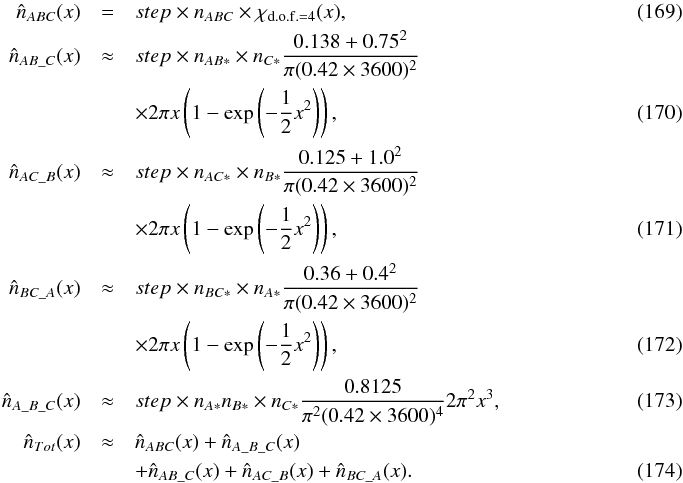 Each component equals step × n × p(s | hi)p(x | hi,s), see Eqs. (111) and (117). We simplify the expression since p(s | hi) ∝ Ik,n(kγ) and p(x | hi,s) ∝ 1 /Ik,n(kγ). The normalized histograms associated to each component are distributed according to each likelihood p(x | hi,s). Both histograms made from the data and theoretical curves are plotted in Fig. 5. The theoretical results fit very well the result of the Chi-square cross-match based on simulated data.
We also verify that the number of “good” ABC matches we obtain as output of the cross-match is coherent with nABC times the input completeness γ.
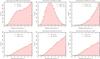 |
Fig. 5 Result of the cross-match of three synthetic catalogues with input values nA = 40 000, nB = 20 000nC = 35 000nAB = 6000, nAC = 12 000, nBC = 18 000 and nABC = 10 000. The error on catalogue A is a constant equal to 0.4′′. The circular error on catalogue B follows a linear distribution between 0.8 and 1.2′′. The circular error on catalogue C follows a Gaussian distribution of mean 0.75′′ and standard deviation of 0.1′′ between 0.5 and 1′′. The common surface area is a cone of radius 0.42°. Top left: histogram of all associations and theoretical curve from the input parameters. Top centre: histogram of real associations and theoretical curve from input parameters. Top right: histogram of “fully” spurious associations and theoretical curve from input paramameters. Bottom: histograms and theoretical curves of associations mixing a real association between two sources plus a spurious source. |
When cross-matching real catalogues, the number of sources nABC, etc. are not known. But the previous “theoretical” curves can be built after a χ-match from the number of sources estimated to compute priors in Sect. 7.
13. Summarized recipe
In this section, we give the main steps and equations to perform a χ-match and to compute for each association the probability it has to be a good match (or any other possible hypothesis).
For a small and compact sky area, project all the sources of all catalogues on an Euclidian plane using for example the ARC projection (Calabretta & Greisen 2002).
To select matching candidates, for each possible set of n sources from n distinct catalogues:
-
compute their weighted mean position (Eq. (30)) andthe associated error (Eq. (29));
-
derive x, the Mahalanobis distance defined by the square root of Eq. (36);
-
fix a constant threshold on all Mahalanobis distances, that is
-
set the fraction α of real associations it is acceptable to miss – the type I error – and
-
derive numerically the threshold kγ inverting Eq. (46) based on the Chi-square distribution with 2(n−1) degrees of freedom (the result is the same computing the threshold from the Chi distribution with 2(n−1) degrees of freedom);
-
To compute Bayes’ probabilities, as many hypotheses as the number of possible partitions of the set of n sources (see Eq. (73), Table 2 and Fig. 1) have to be formulated. Depending on whether one wants to be able to account for photometry in a second step or not, a set of likelihoods may be chosen among several such sets.
In the first case, the likelihood associated to each hypothesis (knowing the selection criteria is fulfilled) depends only on the Mahalanobis distance and on the number of real sources k in the hypothesis hi (see e.g. Fig. 4). The likelihoods are (Eq. (117))  (175)with Ik,n(kγ) given in Eq. (110). The formulae of Ik,n(kγ) and dIk,n(x) are provided for n ≤ 5 in Tables 3 and 4 respectively.
In the second case (no photometry to be taken into account), one can use likelihoods defined by Eq. (146).
Finally, to apply Bayes’ formula, priors p(hi | s) are needed. This is more tricky and the steps detailed in Sect. 7 have to be considered. A pre-requisite is to work on an area (Ω) uniformly covered by all catalogues. For two catalogues, the number of spurious associations can be estimated by computing for each catalogue the mean area covered by the error ellipses for a radius equal to the threshold kγ (so the mean area of the 1σ error ellipses times ). The two means are summed and the result is divided by Ω to obtain the mean probability to spuriously associate two unrelated sources. It is then multiplied by the product of the number of sources in both catalogues to finally obtain the mean expected number of spurious associations (Eq. (85)). Knowing the number of associations in the cross-correlation output, both the probability that one such association is spurious and the complementary probability of having a real association (the two priors of the two-catalogues cross-match) can be estimated (see Eqs. (93) and (94)). Similarly, performing all possible sub-χ-matches, all priors needed for a n-catalogues cross-match can be derived.
All needed ingredients to compute the probabilities associated with each hypothesis are thus available. Those probabilities can be computed applying Eq. (113).
14. Conclusions
In this paper we developed a comprehensive framework for performing the cross-correlation of multiple astronomical catalogues, in one pass. The approach employs a classical χ2-test to select candidates. We computed two sets of likelihoods based on positions, individual elliptical positional errors and the χ2-test region of acceptance: one that can be mixed without any caution with other parameters such as photometric values; and one for which the naive hypothesis of independence between positional uncertainties and magnitudes has to be tested. We also presented a way to estimate “priors” from the region of acceptance of the χ2-test. Probabilities for each possible hypothesis can thus be computed from those likelihoods and “priors”.
In practice the number of hypotheses, and thus the number of “priors”, increases dramatically with the number of catalogues. To be able to cross-match more than six or seven catalogues, it is necessary to simplify the problem. One possibility consists of merging two catalogues of similar astrometric accuracy and similar wavelength range, considering all matches as non-spurious matches. Doing so we would effectively reduce the number of input catalogues by one.
A large part of the statistical work carried out here depends on the simplifying assumptions made in Sect. 3: perfect astrometrical calibration (no systematic offsets), no proper motions, no clustering and no blending. In real life, the “normalized” distance between two detections of a same source present in two distinct catalogues hardly follows a Rayleigh distribution. The “actual distribution” (in practice it is not easy to build such a distribution since it requires secure identifications) often has a broader tail (see for example Rosen et al. 2016, Fig. 5) and a log-normal distribution may better fit it than the Rayleigh distribution. This is probably due to a combination of causes like small proper motions, imperfect reduction, systematics or bias from the calibration process, under or overestimated errors, etc.
In practice this means that the number of associations missed by the candidate selection criteria (based on Rayleigh) is larger that the chosen theoretical value (γ). We could for example add larger systematics to positional errors. The risk is then to distort (even more) the Rayleigh distribution. We could also try to re-calibrate locally the set of catalogues we want to cross-match, but we need secure identifications to do it properly; for each catalogue, all sources in the local area must have been calibrated at once (to possibly correct for a locally uniform systematic using four simple parameters Δα, Δδ, scale, θ). Those two constraints (having secure identifications and at once calibration) are in practice quite hard to satisfy.
If we re-calibrate using a “secure” population (i.e. a population of objects having no proper motions like QSOs) we introduce a bias since QSOs are fainter than most stars in the optical and thus have errors larger than the global population of objects. And adding stars, we introduce noise due to proper motions.
For these reasons, we believe that in case of “old” optical surveys based on photographic plates, a classical fixed radius cross-match may be more efficient that the χ-match to select candidates. We are nonetheless conviced that the equations we derived in this paper can help in building new catalogues, based for example on both multi-band and multi-epoch observations, and can be used to assess and improve the quality of coming surveys.
We generated and processed synthetical catalogues, which meet the simplifying assumptions, in the tool we developed for the ARCHES project. The consistency between the theoretical results derived in this paper – completeness of the candidate selection criterion, likelihoods and priors – and the outputs of the tool has allowed us to cross-validate both the method and its implementation. The tool has also been used to generate ARCHES products which were used in the scientific work packages of the project. Currently the CDS XMatch Service (Pineau et al. 2011a; Boch et al. 2012; Pineau et al. 2015) provides a basic but very efficient facility to cross-correlate two possibly large (>1 billion sources) catalogues. It is planned to include the ARCHES tool into the CDS XMatch. This paper will be the basic reference for the extension of the latter to multi-catalogue statistical χ-match.
From the 2MASS on-line user’s guide http://www.ipac.caltech.edu/2mass/releases/allsky/doc/sec2_2a.html
Original figure: https://commons.wikimedia.org/wiki/File:Set_partitions_5;_cirlces.svg
Acknowledgments
A large part of this work was supported by the ARCHES project. ARCHES (No. 313146) was funded by the 7th Framework of the European Union and coordinated by the University of Strasbourg. All figures (except Fig. 1) were made using the ctioga2 plotting program developped by Vincent Fourmond. F. J. Carrera also acknowledges financial support through grant AYA2015-64346-C2-1-P (MINECO/FEDER).
References
- Adorf, H.-M., Lemson, G., & Voges, W. 2006, in Astronomical Data Analysis Software and Systems XV, eds. C. Gabriel, C. Arviset, D. Ponz, & S. Enrique, ASP Conf. Ser., 351, 695 [Google Scholar]
- Ahn, C. P., Alexandroff, R., Allen de Prieto, C., et al. 2012, ApJS, 203, 21 [NASA ADS] [CrossRef] [Google Scholar]
- Ahn, C. P., Alexandroff, R., Allende Prieto, C., et al. 2013, VizieR Online Data Catalog: V/139 [Google Scholar]
- Aihara, H., Allen de Prieto, C., An, D., et al. 2011, ApJS, 193, 29 [NASA ADS] [CrossRef] [Google Scholar]
- Bertin, E., & Arnouts, S. 1996, A&AS, 117, 393 [NASA ADS] [CrossRef] [EDP Sciences] [Google Scholar]
- Boch, T., Pineau, F., & Derriere, S. 2012, in Astronomical Data Analysis Software and Systems XXI, eds. P. Ballester, D. Egret, & N. P. F. Lorente, ASP Conf. Ser. 461, 291 [Google Scholar]
- Brusa, M., Zamorani, G., Comastri, A., et al. 2007, ApJS, 172, 353 [NASA ADS] [CrossRef] [Google Scholar]
- Budavári, T., & Szalay, A. S. 2008, ApJ, 679, 301 [NASA ADS] [CrossRef] [PubMed] [Google Scholar]
- Calabretta, M. R., & Greisen, E. W. 2002, A&A, 395, 1077 [NASA ADS] [CrossRef] [EDP Sciences] [Google Scholar]
- Cutri, R. M., Skrutskie, M. F., van Dyk, S., et al. 2003, VizieR Online Data Catalog:II/246, 0 [Google Scholar]
- Cutri, R. M., et al. 2014, VizieR Online Data Catalog: II/328 [Google Scholar]
- Fioc, M. 2014, A&A, 566, A8 [NASA ADS] [CrossRef] [EDP Sciences] [Google Scholar]
- Helfand, D. J., White, R. L., & Becker, R. H. 2015a, ApJ, 801, 26 [NASA ADS] [CrossRef] [Google Scholar]
- Helfand, D. J., White, R. L., & Becker, R. H. 2015b, VizieR Online Data Catalog:8 VIII/092 [Google Scholar]
- Høg, E., Fabricius, C., Makarov, V. V., et al. 2000, A&A, 355, L27 [Google Scholar]
- Hsu, L.-T., Salvato, M., Nandra, K., et al. 2014, ApJ, 796, 60 [NASA ADS] [CrossRef] [Google Scholar]
- Inglot, T. 2010, Prob. Math. Stat., 30, 339 [Google Scholar]
- Lasker, B., Lattanzi, M. G., McLean, B. J., et al. 2007, VizieR Online Data Catalog: I/305 [Google Scholar]
- Lasker, B. M., Lattanzi, M. G., McLean, B. J., et al. 2008, AJ, 136, 735 [NASA ADS] [CrossRef] [PubMed] [Google Scholar]
- Menzel, M.-L., Merloni, A., Georgakakis, A., et al. 2016, MNRAS, 457, 110 [NASA ADS] [CrossRef] [Google Scholar]
- Mingo, B., Watson, M. G., Rosen, S. R., et al. 2016, MNRAS, 462, 2631 [NASA ADS] [CrossRef] [Google Scholar]
- Motch, C., Carrera, F. J., Genova, F., et al. 2016, in Astronomical Data Analysis Software an Systems XXV (ADASS XXV), eds. F. Lorente & E. Shortridge, ASP Conf. Ser. [arXiv:1609.00809] [Google Scholar]
- Naylor, T., Broos, P. S., & Feigelson, E. D. 2013, ApJS, 209, 30 [NASA ADS] [CrossRef] [Google Scholar]
- Pier, J. R., Munn, J. A., Hindsley, R. B., et al. 2003, AJ, 125, 1559 [NASA ADS] [CrossRef] [Google Scholar]
- Pineau, F.-X., Boch, T., & Derriere, S. 2011a, in Astronomical Data Analysis Software and Systems XX, eds. I. N. Evans, A. Accomazzi, D. J. Mink, & A. H. Rots, ASP Conf. Ser., 442, 85 [Google Scholar]
- Pineau, F.-X., Motch, C., Carrera, F., et al. 2011b, A&A, 527, A126 [NASA ADS] [CrossRef] [EDP Sciences] [Google Scholar]
- Pineau, F., Boch, T., Derriere, S., & Arches Consortium. 2015, in Astronomical Data Analysis Software an Systems XXIV (ADASS XXIV), eds. A. R. Taylor, & E. Rosolowsky, ASP Conf. Ser., 495, 61 [Google Scholar]
- Press, W. H., Teukolsky, S. A., Vetterling, W. T., & Flannery, B. P. 2007, Numerical Recipes, The Art of Scientific Computing, 3rd edn. (New York: Cambridge University Press) [Google Scholar]
- Richards, G. T., Nichol, R. C., Gray, A. G., et al. 2004, ApJS, 155, 257 [NASA ADS] [CrossRef] [Google Scholar]
- Rosen, S. R., Webb, N. A., Watson, M. G., et al. 2016, A&A, 590, A1 [NASA ADS] [CrossRef] [EDP Sciences] [Google Scholar]
- Rutledge, R. E., Brunner, R. J., Prince, T. A., & Lonsdale, C. 2000, ApJS, 131, 335 [NASA ADS] [CrossRef] [Google Scholar]
- Rutledge, R. E., Fox, D. W., Bogosavljevic, M., & Mahabal, A. 2003, ApJ, 598, 458 [NASA ADS] [CrossRef] [Google Scholar]
- Skrutskie, M. F., Cutri, R. M., Stiening, R., et al. 2006, AJ, 131, 1163 [NASA ADS] [CrossRef] [Google Scholar]
- Stuart, A., & Ord, K. 1994, Kendall’s Advanced Theory of Statistics: Volume 1: Distribution Theory, Kendall’s advanced theory of statistics (Wiley) [Google Scholar]
- Taylor, M. B. 2005, in Astronomical Data Analysis Software and Systems XIV, eds. P. Shopbell, M. Britton, & R. Ebert, ASP Conf. Ser., 347, 29 [Google Scholar]
- Voges, W., Aschenbach, B., Boller, T., et al. 1999, A&A, 349, 389 [NASA ADS] [Google Scholar]
- Watson, M. 2012, in Half a Century of X-ray Astronomy, Proc. Conference held 17–21 September, 2012 in Mykonos Island, Greece, 138 [Google Scholar]
- White, R. L., Becker, R. H., Helfand, D. J., & Gregg, M. D. 1997, ApJ, 475, 479 [NASA ADS] [CrossRef] [Google Scholar]
- White, N. E., Giommi, P., & Angelini, L. 2000, VizieR Online Data Catalog: VIII/031 [Google Scholar]
- Wolstencroft, R. D., Savage, A., Clowes, R. G., et al. 1986, MNRAS, 223, 279 [NASA ADS] [Google Scholar]
- Wright, E. L., Eisenhardt, P. R. M., Mainzer, A. K., et al. 2010, AJ, 140, 1868 [Google Scholar]
- Zacharias, N., Urban, S. E., Zacharias, M. I., et al. 2004, AJ, 127, 3043 [NASA ADS] [CrossRef] [Google Scholar]
Appendix A: Demonstrations
Appendix A.1: From V to VΣ
to VΣ
From Eq. (28), we compute for 2 × 2 symmetric square matrices:  in which adjA is the adjugate matrix of A, that is the transpose of the cofactor matrix of A.
Appendix A.2: Sum of quadratics canonical form
First expanding and then factoring:  We use
 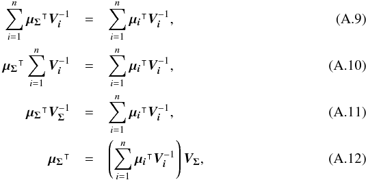 that we introduce in the previous equations to finally find
 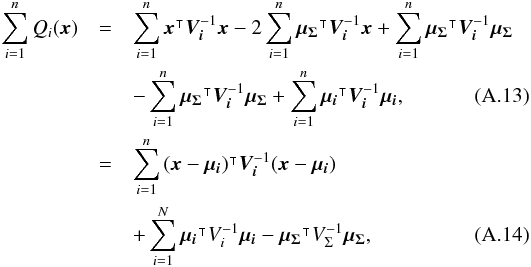 or,
or, 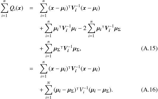
Appendix A.3: Expanding the Qχ2 term
Noting that 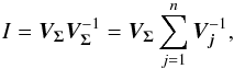 (A.17)we can write
 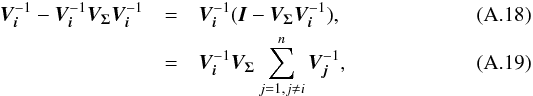 and thus, with square symmetric matrices:
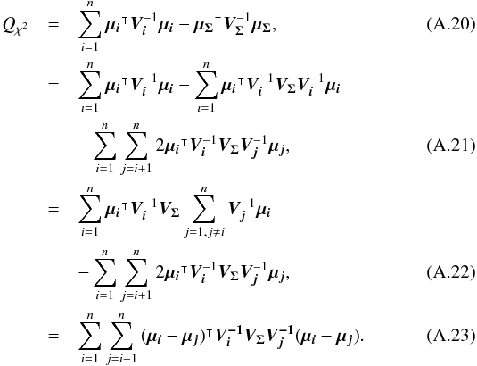
Appendix A.4: Sum of 2 quadratics: Qχ term
We first develop: ![Mathematical equation: \appendix \setcounter{section}{1} \begin{eqnarray} \transposee{\vec{\mu_{\Sigma_2}}}\bm{V_{\Sigma_2}}^{-1}\vec{\mu_{\Sigma_2}} & = & (\transposee{\vec{\mu_1}}\bm{V_1}^{-1} + \transposee{\vec{\mu_2}}\bm{V_2}^{-1})V_{\Sigma_2} \nonumber \\ & & \times \left(\bm{V_1}^{-1}\vec{\mu_1} + \bm{V_2}^{-1}\vec{\mu_2}\right), \\ & = & \left(\transposee{\vec{\mu_1}}\bm{V_1}^{-1} + \transposee{\vec{\mu_2}}\bm{V_2}^{-1}\right) \frac{1}{|\frac{\bm{V_1}}{|\bm{V_1}|} + \frac{\bm{V_2}}{|\bm{V_2}|}|} \nonumber \\ & &\times \left(\frac{\bm{V_1}}{|\bm{V_1}|} + \frac{\bm{V_2}}{|\bm{V_2}|}\right) \left(\bm{V_1}^{-1}\vec{\mu_1} + \bm{V_2}^{-1}\vec{\mu_2}\right), \\ & = & |\bm{V_{\Sigma_2}}|\left[\transposee{\vec{\mu_1}}\frac{\bm{V_1}^{-1}}{|\bm{V_1}|}\vec{\mu_1} + \transposee{\vec{\mu_2}}\frac{\bm{V_2}^{-1}}{|\bm{V_2}|}\vec{\mu_2}\right. \nonumber \\ & & + \left.\transposee{\vec{\mu_1}}\frac{\bm{V_2}^{-1}}{|\bm{V_1}|}\vec{\mu_2} + \transposee{\vec{\mu_2}}\frac{\bm{V_1}^{-1}}{|\bm{V_2}|}\vec{\mu_1} \right] \nonumber \\ & & +|\bm{V_{\Sigma_2}}|\left[\transposee{\vec{\mu_1}}\frac{\bm{V_1}^{-1}}{|\bm{V_2}|}\vec{\mu_2} + \transposee{\vec{\mu_2}}\frac{\bm{V_2}^{-1}}{|\bm{V_1}|}\vec{\mu_1}\right. \nonumber \\ & & + \transposee{\vec{\mu_1}}\bm{V_1}^{-1}\frac{\bm{V_2}}{|\bm{V_2}|}\bm{V_1}^{-1}\vec{\mu_1} \nonumber \\ & & + \left.\transposee{\vec{\mu_2}}\bm{V_2}^{-1}\frac{\bm{V_1}}{|\bm{V_1}|}\bm{V_2}^{-1}\vec{\mu_2}\right]. \end{eqnarray}](/articles/aa/full_html/2017/01/aa29219-16/aa29219-16-eq585.png) Computing
Computing  :
: 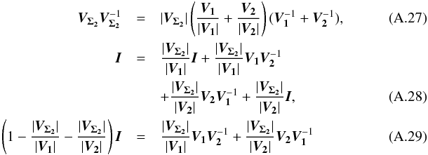 We can write:
 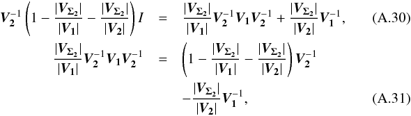 and, similarly:
 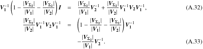 We use the above 3 relations to develop
  (A.34)which leads to
  (A.35)Using Eq. (52) we found that
  (A.36)is equal to
  (A.37)
Appendix A.5: χ and χ2 distributions
Appendix A.5.1: Definition
The χ and χ2 distributions with k = 2(n−1) degrees of freedom are defined as 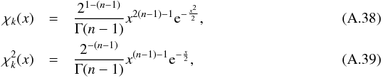 with the gamma function ∀l ∈N, Γ(l) = (l−1) ! it leads to
 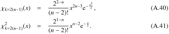 So for
 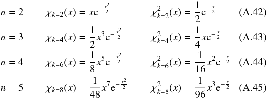 and so on.
Appendix A.5.2: Sum of two χ functions
We show here that χk = 2p(x1) + χk = 2q(x2) = χk = 2(p + q)(x). The distribution we are looking for is the density function of χk = 2p(x1)χk = q(x2)dx1dx2 given  . We use polar coordinates so, dx1dx2 = xdxdθ, x1 = xcosθ and x2 = xsinθ:
 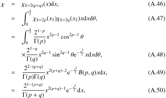 in which B(p,q) is the beta function
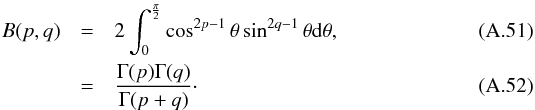
Appendix A.5.3: χk = 2(n−1) cumulative distribution function
Directly integrating for k = 2![Mathematical equation: \appendix \setcounter{section}{1} \begin{equation} F_{\rchi_{k=2}}(x) = \int_0^x \rchi_{k=2}(x')\mathrm{d}x' = \left[-{\rm e}^{-\frac{1}{2}x'^2}\right]_0^x = 1 - {\rm e}^{-\frac{1}{2}x^2} \end{equation}](/articles/aa/full_html/2017/01/aa29219-16/aa29219-16-eq611.png) (A.53)For k = 4, we integrate by parts with
(A.53)For k = 4, we integrate by parts with 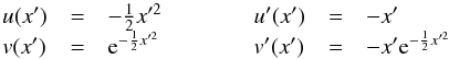 (A.54)so
 ![Mathematical equation: \appendix \setcounter{section}{1} \begin{eqnarray} F_{\rchi_{k=4}}(x) & = & \int_0^x \rchi_{k=4}(x')\mathrm{d}x', \\ & = & F_{\rchi_{k=2}}(x) + \left[-\frac{1}{2}x'^2{\rm e}^{-\frac{1}{2}x'^2}\right]_0^x, \\ & = & F_{\rchi_{k=2}}(x) - \frac{1}{2}x^2 {\rm e}^{-\frac{1}{2}x^2}. \end{eqnarray}](/articles/aa/full_html/2017/01/aa29219-16/aa29219-16-eq613.png) For k = 6, also integrating by parts, we note
For k = 6, also integrating by parts, we note  (A.58)and so
 ![Mathematical equation: \appendix \setcounter{section}{1} \begin{eqnarray} F_{\rchi_{k=6}}(x) & = & \int_0^x \rchi_{k=6}(x')\mathrm{d}x', \\ & = & F_{\rchi_{k=4}}(x) + \left[-\frac{1}{8}x'^4{\rm e}^{-\frac{1}{2}x'^2}\right]_0^x, \\ & = & F_{\rchi_{k=4}}(x) - \frac{1}{8}x^4 {\rm e}^{-\frac{1}{2}x^2}. \end{eqnarray}](/articles/aa/full_html/2017/01/aa29219-16/aa29219-16-eq616.png) We deduce the general form for k = 2(n−1):
We deduce the general form for k = 2(n−1): 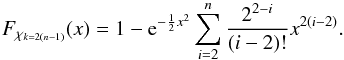 (A.62)
Appendix A.6: Computing the Ik,n(x) integral
Let us first expand a few notations for a better readability 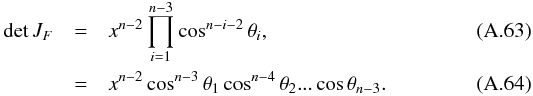 We are supposed to use | detJF | but x is positive and all angles θ are ∈ [0,π/ 2], so detJF is always positive. Let us also expand
 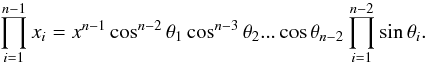 (A.65)Multiplying both expressions leads to
 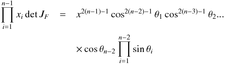 (A.66)
Appendix A.6.1: Case Ik=1,n(x)
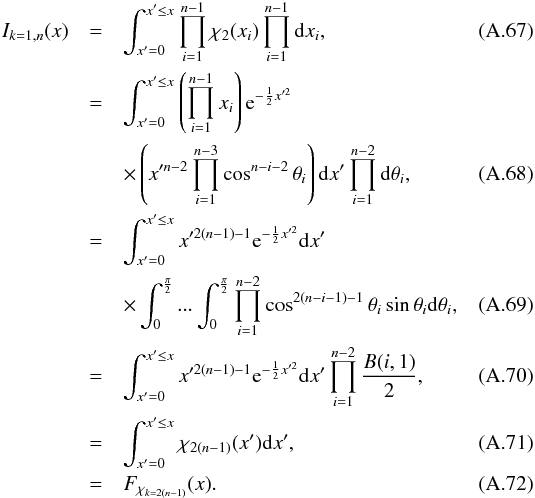 The exact solution is given by Eq. (A.62).
We note the particular case Ik,n(kγ) = γ if kγ computed for this particular value of n.
Appendix A.6.2: Case Ik=n,n(x)
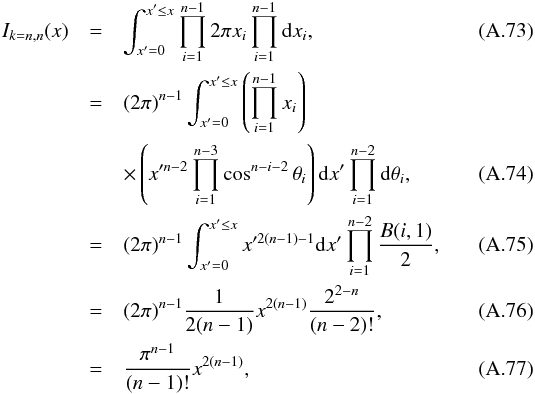 which is the volume of an hypersphere of dimension 2(n−1), also called 2(n−1)-sphere.
Appendix A.6.3: Intermediate case Ik,n(x)
For k> 1 and k<n: 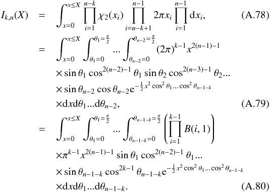 In a first step, we integrated by parts using
 ![Mathematical equation: \appendix \setcounter{section}{1} \begin{eqnarray} u(\theta_{n-1-k}) & = & \cos^{2(k-1)}\theta_{n-1-k}, \\ u'(\theta_{n-1-k}) & = & -2(k-1)\sin\theta_{n-1-k}\cos^{2(k-1)-1}\theta_{n-1-k}, \\ c^2 & = & \cos^2\theta_1...\cos^2\theta_{n-2-k}, \\ v(\theta_{n-1-k}) & = & {\rm e}^{-\frac{1}{2}x^2c^2\cos^2\theta_{n-1-k}}, \\ v'(\theta_{n-1-k}) & = & x^2 c^2 \sin\theta_{n-1-k}\cos\theta_{n-1-k} {\rm e}^{-\frac{1}{2}x^2c^2\cos^2\theta_{n-1-k}}, \\ \left[uv\right]_0^{\pi/2} & = & -{\rm e}^{-\frac{1}{2}x^2c^2}, \\ -\int_0^{\frac{\pi}{2}} u'v & = & \int 2(k-1)\sin\theta_{n-1-k}\cos^{2(k-1)-1}\theta_{n-1-k} \nonumber\\ & & \times {\rm e}^{-\frac{1}{2}x^2c^2\cos^2\theta_{n-1-k}}\mathrm{d}\theta_{n-1-k}. \end{eqnarray}](/articles/aa/full_html/2017/01/aa29219-16/aa29219-16-eq634.png) We thus find that
We thus find that ![Mathematical equation: \appendix \setcounter{section}{1} \begin{eqnarray} I_{k, n}(X) & = & \int_{x=0}^{x \le X} \int_{\theta_1=0}^{\theta_1=\frac{\pi}{2}}... \int_{\theta_{n-(k+2)}=0}^{\theta_{n-(k+2)}=\frac{\pi}{2}} \frac{1}{(k-1)!}\pi^{k-1}x^{2(n-2)-1} \nonumber \\ & & \times \sin\theta_1\cos^{2(n-3)-1}\theta_1... \sin\theta_{n-2-k}\cos^{2k-1}\theta_{n-2-k} \nonumber \\ & & \times\left[\int u'v \mathrm{d}\theta_{n-1-k} - {\rm e}^{-\frac{1}{2}x^2c^2} \right] \mathrm{d}x\mathrm{d}\theta_1...\mathrm{d}\theta_{n-2-k}. \end{eqnarray}](/articles/aa/full_html/2017/01/aa29219-16/aa29219-16-eq635.png) (A.88)We finally find the recurrence formula
(A.88)We finally find the recurrence formula  (A.89)since
 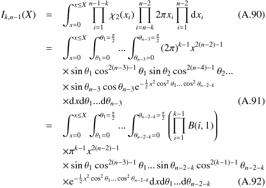 and
and 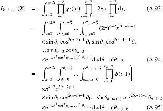 Knowing that
  (A.96)we integrate the differents parts:
Appendix B: Proper motion estimation and testing
Appendix B.1: Estimating proper motions
In this section, we show how it is possible to estimate the proper motion v of a source if the simplifying assumption of null proper motion made in Sect. 3 is not met. We neglect the parallax and the long term effect of the radial motion of the source, but those extra parameters could also be fitted provided we have enough catalogue measurements. In our simple case, the position p of a source at any time t can be computed from its position p0 at a reference epoch (e.g. 2000):  (B.1)We assume we have n observations of the source at various epochs ti. We want to estimate the proper motion, so to estimate the 4 unknowns (vx,vy,x0,y0). To do so we use the maximum-likelihood estimate which consists in maximizing the likelihood
 (B.2)therefore minimizing
  (B.3)by solving the system of equations
  (B.4)To do so, we compute the derivative of χ2(p(t)) according to a parameter ak
![Mathematical equation: \appendix \setcounter{section}{2} \begin{eqnarray} \frac{\partial \rchi^2(\vec{p}(t))}{\partial a_k} & = & -2\sum\limits_{i=1}^n \frac{1}{(1-\rho_i^2)}\left[ \frac{(\mu_{i_x} - p_x)}{\sigma_{i_x}^2}\frac{\partial p_x}{\partial a_k} + \frac{(\mu_{i_y} - p_y)}{\sigma_{i_y}^2}\frac{\partial p_y}{\partial a_k} \right. \nonumber \\ & & \left. - \frac{\rho_i}{\sigma_{i_x}\sigma_{i_y}}\left( (\mu_{i_y} - p_y)\frac{\partial p_x}{\partial a_k} + (\mu_{i_x} - p_x)\frac{\partial p_y}{\partial a_k} \right) \right], \label{eq:dkhi2} \end{eqnarray}](/articles/aa/full_html/2017/01/aa29219-16/aa29219-16-eq652.png) (B.5)and the Jacobian matrix of p(t | v,p0)
(B.5)and the Jacobian matrix of p(t | v,p0)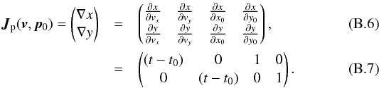 So we have to solve the following system of equations, noting Δti = ti−t0
![Mathematical equation: \appendix \setcounter{section}{2} \begin{equation} \left\{ \begin{array}{lclr} \sum\limits_{i=1}^n\frac{1}{(1-\rho_i^2)}\left[ \frac{(\mu_{i_x} - x)}{\sigma_{i_x}^2} - \frac{\rho_i}{\sigma_{i_x}\sigma_{i_y}}(\mu_{i_y} - y) \right] \Delta t_i & = & 0 & (a),\\ \sum\limits_{i=1}^n\frac{1}{(1-\rho_i^2)}\left[ \frac{(\mu_{i_y} - y)}{\sigma_{i_y}^2} - \frac{\rho_i}{\sigma_{i_x}\sigma_{i_y}}(\mu_{i_x} - x) \right] \Delta t_i & = & 0 & (b),\\ \sum\limits_{i=1}^n\frac{1}{(1-\rho_i^2)}\left[ \frac{(\mu_{i_x} - x)}{\sigma_{i_x}^2} - \frac{\rho_i}{\sigma_{i_x}\sigma_{i_y}}(\mu_{i_y} - y) \right] & = & 0 & (c), \\ \sum\limits_{i=1}^n\frac{1}{(1-\rho_i^2)}\left[ \frac{(\mu_{i_y} - y)}{\sigma_{i_y}^2} - \frac{\rho_i}{\sigma_{i_x}\sigma_{i_y}}(\mu_{i_x} - x) \right] & = & 0 & (d). \end{array} \right. \end{equation}](/articles/aa/full_html/2017/01/aa29219-16/aa29219-16-eq656.png) (B.8)We can for example use Cramer’s rule to solve the general problem
(B.8)We can for example use Cramer’s rule to solve the general problem  (B.9)with, in our case, and using the notation
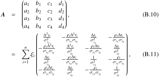
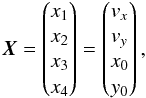 (B.12)and
 ![Mathematical equation: \appendix \setcounter{section}{2} \begin{equation} \vec{\Lambda} = \begin{pmatrix} e_1 \\ e_2 \\ e_3 \\ e_4 \end{pmatrix} = \begin{pmatrix} \sum\limits_{i=1}^N\xi_i\left[ \frac{\mu_{i_x}}{\sigma_{i_x}^2} - \frac{\rho_i\mu_{i_y}}{\sigma_{i_x}\sigma_{i_y}} \right] \Delta t_i \\ \sum\limits_{i=1}^N\xi_i\left[ \frac{\mu_{i_y}}{\sigma_{i_y}^2} - \frac{\rho_i\mu_{i_x}}{\sigma_{i_x}\sigma_{i_y}} \right] \Delta t_i \\ \sum\limits_{i=1}^N\xi_i\left[ \frac{\mu_{i_x}}{\sigma_{i_x}^2} - \frac{\rho_i\mu_{i_y}}{\sigma_{i_x}\sigma_{i_y}} \right] \\ \sum\limits_{i=1}^N\xi_i\left[ \frac{\mu_{i_y}}{\sigma_{i_y}^2} - \frac{\rho_i\mu_{i_x}}{\sigma_{i_x}\sigma_{i_y}} \right] \end{pmatrix}, \end{equation}](/articles/aa/full_html/2017/01/aa29219-16/aa29219-16-eq661.png) (B.13)leading to the solution
(B.13)leading to the solution  (B.14)where
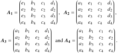
Appendix B.2: Estimating the error on the proper motion estimate
The covariance matthat isVf on the estimated proper motion parameters is provided by the inverse of the Hessian matrix Hf of  , evaluated with the estimated parameters, that is by the matrix
 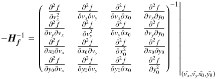 (B.15)
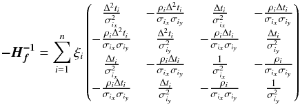 (B.16)
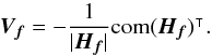 (B.17)
Appendix B.3: Simple case: no covariance
If all positional errors are circles (i.e. ∀i ∈ [1,n] ,ρi = 0), the simplifications leads to the classical formulae in which x and y are computed independently (see Press et al. 2007, p. 781, Sect. 15.2 “Fitting Data to a Straight Line”) 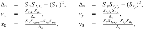 (B.18)where
 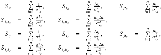 (B.19)and associated errors are
 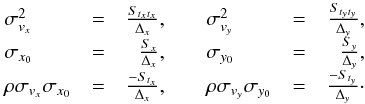 (B.20)
Appendix B.4: Verifying the results
We have implemented and tested the result given by equation Eq. (B.14). We compare the results with a modified version of the Levenberg-Marquardt (LM) method (see Press et al. 2007, p. 801, Sect. 15.5.2 “Levenberg-Marquardt method”) we designed tohandle binormal distributions. The algorithm is the same except that we replace the term  in βk by Eq. (B.5) and αkl by
 ![Mathematical equation: \appendix \setcounter{section}{2} \begin{eqnarray} \sum\limits_{i=1}^n\frac{1}{(1-\rho_i^2)} & & \left[ \frac{1}{\sigma_{i_x}^2} \frac{\partial p_x}{\partial a_k}\frac{\partial p_x}{\partial a_l} + \frac{1}{\sigma_{i_y}^2} \frac{\partial p_y}{\partial a_k}\frac{\partial p_y}{\partial a_l} \right. \nonumber \\ & & \left. - \frac{\rho_i}{\sigma_{i_x}\sigma_{i_y}} \left( \frac{\partial p_x}{\partial a_k}\frac{\partial p_y}{\partial a_l} - \frac{\partial p_y}{\partial a_k}\frac{\partial p_x}{\partial a_l} \right) \right]\cdot \end{eqnarray}](/articles/aa/full_html/2017/01/aa29219-16/aa29219-16-eq677.png) (B.21)We initialize the LM parameters with the approximate solutions given in Eq. (B.18). The results obtained using both methods (LM and Eq. (B.14)) are identical.
(B.21)We initialize the LM parameters with the approximate solutions given in Eq. (B.18). The results obtained using both methods (LM and Eq. (B.14)) are identical.
Appendix B.5: Testing the unique source hypothesis
When estimating the proper motion, we formulated the hypothesis H than our n observations come from a single underlying source. The Chi-square of equation Eq. (B.3) follows a Chi-square distribution with 2n−4 = 2(n−2) degrees of freedom. Therefore the criteria not to reject H is 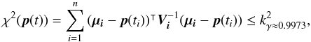 (B.22)in which
 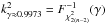 .
.
Appendix C: Synthetic catalogues generation script
Here is the script used to generate three synthetical tables and cross-match them with the online ARCHES XMatch Tool. The language of the script is specific to the tool. Both the tool and its documentation are available online10.
synthetic seed=1 nTab=3 prefix=true \
  geometry=cone ra=22.5 dec=33.5 r=0.42 \
  nA=40000 nB=20000 nC=35000 \
  nAB=6000 nAC=12000 nBC=18000 \
  nABC=10000 \
  poserrAtype=CIRCLE poserrAmode=formula paramA1=0.4 \
  poserrBtype=CIRCLE poserrBmode=function paramB1func=x \
                     paramB1xmin=0.8 paramB1xmax=1.2 \
                     paramB1nstep=100 \
  poserrCtype=CIRCLE poserrCmode=function \
                     paramC1func=exp(-0.5*(x-0.75)*(x-0.75)/0.01)/(0.1*sqrt(2*PI)) \
                     paramC1xmin=0.5 paramC1xmax=1 \
                     paramC1nstep=100
save prefix=simu3 suffix=.fits common=simu3.fits format=fits

cleartables

get FileLoader file=simu3A.fits
set pos ra=posRA dec=posDec
set poserr type=CIRCLE param1=ePosA param2=ePosB param3=ePosPA
set cols *

get FileLoader file=simu3B.fits
set pos ra=posRA dec=posDec
set poserr type=CIRCLE param1=ePosA param2=ePosB param3=ePosPA
set cols *

xmatch chi2 completeness=0.9973 nStep=1 nMax=2 join=inner
merge pos chi2
merge dist mec

get FileLoader file=simu3C.fits
set pos ra=posRA dec=posDec
set poserr type=CIRCLE param1=ePosA param2=ePosB param3=ePosPA
set cols *

xmatch chi2 completeness=0.9973 nStep=2 nMax=2 join=inner
merge pos chi2
merge dist mec

save simu3.ABC.fits fits
All Tables
Summary of the transformations of positional errors provided in various astronomical catalogues into the coefficients of error covariance matrices (before adding quadratically possible systematics).
Values of the normalization integrals Ik,n−k(kγ) for a number of catalogue ranging from two to five.
Values of the derivatives of normalization integrals for a number of catalogue ranging from two to five.
All Figures
|
Fig. 1 The 52 partitions of a set with n = 5 elements. Each partition corresponds to one hypothesis for five distinct sources from five distinct catalogues. Left: k = 5, the five sources are from five distinct real sources. Right: k = 1, the five sources are from a same real source. (Tilman Piesk – CC BY 3.0 – modified – link in footnote). |
| In the text | |
|
Fig. 2 Two possible likelihoods for n = 2 catalogues and γ = 0.9973: normalized Rayleigh (red, filled curve) and Poisson (green, dashed curve) components. We note that this γ value implies the [0,kγ = 3.443935] range for x. |
| In the text | |
|
Fig. 3 Three possible likelihoods p(x | hk,s) for n = 3 catalogues and γ = 0.9973: χ distribution with four degrees of freedom (red, filled curve); Integral of a χ distribution with two degrees of freedom times a two-dimensional Poisson distribution (green, dashed curve); Four-dimensional Poisson distribution (blue, dotted curve). |
| In the text | |
|
Fig. 4 Four possible likelihoods p(x | hk,s) for n = 4 catalogues and γ = 0.9973: χ distribution with six degrees of freedom (red, filled curve); integral of a χ distribution with two degrees of freedom times a four-dimensional Poisson distribution (green, dashed curve); integral of a χ distribution with four degrees of freedom times a two-dimensional Poisson distribution (blue, dotted curve); six-dimensional Poisson distribution (cyan, filled curve). |
| In the text | |
|
Fig. 5 Result of the cross-match of three synthetic catalogues with input values nA = 40 000, nB = 20 000nC = 35 000nAB = 6000, nAC = 12 000, nBC = 18 000 and nABC = 10 000. The error on catalogue A is a constant equal to 0.4′′. The circular error on catalogue B follows a linear distribution between 0.8 and 1.2′′. The circular error on catalogue C follows a Gaussian distribution of mean 0.75′′ and standard deviation of 0.1′′ between 0.5 and 1′′. The common surface area is a cone of radius 0.42°. Top left: histogram of all associations and theoretical curve from the input parameters. Top centre: histogram of real associations and theoretical curve from input parameters. Top right: histogram of “fully” spurious associations and theoretical curve from input paramameters. Bottom: histograms and theoretical curves of associations mixing a real association between two sources plus a spurious source. |
| In the text | |
Current usage metrics show cumulative count of Article Views (full-text article views including HTML views, PDF and ePub downloads, according to the available data) and Abstracts Views on Vision4Press platform.
Data correspond to usage on the plateform after 2015. The current usage metrics is available 48-96 hours after online publication and is updated daily on week days.
Initial download of the metrics may take a while.