| Issue |
A&A
Volume 596, December 2016
|
|
|---|---|---|
| Article Number | A28 | |
| Number of page(s) | 10 | |
| Section | Interstellar and circumstellar matter | |
| DOI | https://doi.org/10.1051/0004-6361/201629039 | |
| Published online | 23 November 2016 | |
Ambipolar diffusion regulated collapse of filaments threaded by perpendicular magnetic fields
1 School of Physics and Astronomy,
University of Leeds, Leeds LS2
9JT, UK
e-mail: This email address is being protected from spambots. You need JavaScript enabled to view it.
2 Department of Applied Mathematics,
University of Leeds, Leeds
LS2 9JT,
UK
Received:
1
June
2016
Accepted:
8
September
2016
Abstract
Context. In giant molecular clouds (GMCs), the fractional ionisation is low enough that the neutral and charged particles are weakly coupled. A consequence of this is that the magnetic flux redistributes within the cloud, allowing an initially magnetically supported region to collapse.
Aims. We aim to elucidate the effects of ambipolar diffusion on the evolution of infinitely long filaments and the effect of decaying turbulence on that evolution.
Methods. First, in ideal magnetohydrodynamics (MHD), a two-dimensional cylinder of an isothermal magnetised plasma with initially uniform density was allowed to evolve to an equilibrium state. Then, the response of the filament to ambipolar diffusion was followed using an adaptive mesh refinement multifluid MHD code. Various ambipolar resistivities were chosen to reflect different ratios of Jeans length to ambipolar diffusion length scale. To study the effect of turbulence on the ambipolar diffusion rate, we perturbed the equilibrium filament with a turbulent velocity field quantified by a rms sonic Mach number, Mrms, of 10, 3 or 1.
Results. We numerically reproduce the density profiles for filaments that are in magnetohydrostatic and pressure equilibrium with their surroundings obtained in a published model and show that these equilibria are dynamically stable. If the effect of ambipolar diffusion is considered, these filaments lose magnetic support initiating cloud collapse. The filaments do not lose magnetic flux. Rather the magnetic flux is redistributed within the filament from the dense centre towards the diffuse envelope. The rate of the collapse is inversely proportional to the fractional ionisation and two gravitationally-driven ambipolar diffusion regimes for the collapse are observed as predicted in a published model. For high values of the ionisation coefficient, that is X ≥ 10-7, the gas is strongly coupled to the magnetic field and the Jeans length is larger than the ambipolar diffusion length scale. Then the collapse is governed by magnetically-regulated ambipolar diffusion. The gas collapses at velocities much lower than the sound speed. For X ≲ 10-8, the gas is weakly coupled to the magnetic field and the magnetic support is removed by gravitationally-dominated ambipolar diffusion. Here, neutrals and ions only collide sporadically, that is the ambipolar diffusion length scale is larger than the Jeans length, and the gas can attain high collapse velocities. When decaying turbulence is included, additional support is provided to the filament. This slows down the collapse of the filament even in the absence of a magnetic field. When a magnetic field is present, the collapse rate increases by a ratio smaller than for the non-magnetic case. This is because of a speed-up of the ambipolar diffusion due to larger magnetic field gradients generated by the turbulence and because the ambipolar diffusion aids the dissipation of turbulence below the ambipolar diffusion length scale. The highest increase in the rate is observed for the lowest ionisation coefficient and the highest turbulent intensity.
Key words: methods: numerical / ISM: magnetic fields / ISM: clouds / stars: formation / magnetohydrodynamics (MHD)
© ESO 2016
1. Introduction
Giant molecular clouds (GMCs) contain regions of enhanced density where star formation occurs. These regions often take the form of structures such as clumps and filaments (e.g. Sakamoto et al. 1994; Engargiola et al. 2003). These structures may be thermally supported, or in cases where the mass of the object exceeds the Jeans mass, a magnetic field can provide support against gravitational collapse, provided that it is sufficiently strong. Only if such structures are able to fragment or collapse into sufficiently dense cores, can protostellar objects form. Various mechanisms for initiating this collapse have been suggested, including collisions between clouds (e.g. Takahira et al. 2014), shock-cloud interactions (e.g. Bonnell et al. 2006; Vaidya et al. 2013), and perturbation of cores by waves (e.g. McKee & Zweibel 1995; Van Loo et al. 2007).
Mestel & Spitzer (1956) suggested that ambipolar diffusion due to the relative motion between the neutrals and ions, can also fragment molecular clouds into dense cores. Detailed calculations of Mouschovias (1976, 1979) subsequently showed that ambipolar diffusion does, indeed, leads to the self-initiated collapse of dense central regions while the cloud envelope remains magnetically supported as magnetic flux is redistributed. Additional numerical simulations of magnetically sub-critical self-gravitating sheets or layers further confirm the ambipolar-diffusion regulated fragmentation process (e.g. Kudoh & Basu 2011, 2014).
In this paper we consider the effect of ambipolar diffusion and velocity perturbations on magnetically sub-critical filaments. In these models the magnetic field is perpendicular to the filament axis. Filamentary clouds threaded by magnetic fields (both parallel and perpendicular to their axis) are expected to form due to gravitational and thermal instabilities within thin dense layers (e.g. Kudoh et al. 2007; Vázquez-Semadeni et al. 2011; Van Loo et al. 2014). Many observed filaments in GMCs exhibit such a configuration (Li et al. 2013), but as yet little theoretical study of such structures has been performed. In Sect. 2 we describe the numerical code and our initial conditions based on the analytic work of Tomisaka (2014). Then, in Sect. 4, we investigate the effect of ambipolar diffusion on the evolution of the filaments. We also examine the interaction of velocity perturbations with the diffusion process in Sect. 5. Finally, in Sect. 6, we discuss and summarise our results.
2. The model
2.1. Multifluid code
Within molecular clouds the fractional ionisation is low, so the gas can be treated as a multispecies fluid consisting of neutrals, electrons and ions. Furthermore, we have adopted an isothermal equation of state p = ρT for all fluids with T the isothermal temperature. For the neutral fluid, the governing isothermal equations are given by 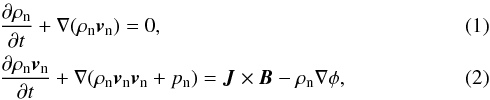 with ρn the neutral density, vn the neutral velocity, pn the neutral pressure, φ the gravitational potential, B the magnetic field and J the current given by J = ∇ × B. As we are interested in the filament configuration and evolution for a given line mass and mass-to-flux ratio, we have only applied the gravitational force ρn∇φ for filament gas to avoid accretion of external gas by the filament. In the limit of small mass densities for the electrons and ions, the gravitational potential can be calculated using the Poisson equation
  (3)here G is the gravitational constant which we set to 1.
For the charged fluids, we assumed ionisation equilibrium (e.g. Elmegreen 1979) and also neglected their inertia so that the equations reduce to  (4)where X is the ionisation coefficient related to the ionisation fraction
  , αj the charge-to-mass ratio, Kjn the collision coefficient of the charged fluid j with the neutrals, and E the electric field. Here j stands for either the electrons or ions. We used 10-6 ≤ X ≤ 10-8 and adopted a charge-to-mass ratio αe = −8.39 × 10¹⁵ for the electrons and αi = 1.52 × 10¹¹ for the ions, and Ken = 2.99 × 10¹⁰ and Kin = 2.06 × 10⁷ as the collision coefficients between the electrons and ions with the neutrals. We assumed an ion mass of 30mH.
If we take a dimensional sound speed within the cloud of 0.35 km s-1 (corresponding to ≈20 K), this equates to a cloud radius of ≈0.3 pc (consistent with observed filament widths; André et al. 2010).
We have also included the effects of ambipolar diffusion. Using the charged fluid momentum equation to substitute E in the Maxwell-Faraday equation, the evolution of the magnetic field is governed by 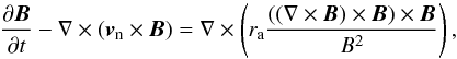 (5)where we have neglected the contributions of the resistivity along the field and the Hall resistivity. This can be done as the Hall parameter for electrons and ions are much larger than unity. Furthermore, as the Hall parameter for electrons is larger than that for ions, ra (the ambipolar resistivity) is given by (Falle 2003)
 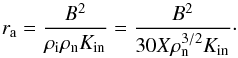 (6)These equations are solved using the multifluid version of the adaptive mesh refinement code MG, which is described in detail in Van Loo et al. (2008) and based on the algorithms outlined in Falle (2003). This scheme uses a second-order Godunov solver with a linear Riemann solver for the neutral fluid equations. The charged fluid velocities can be calculated from the reduced momentum equation and the magnetic field is advanced explicitly which imposes an extra restriction on the stable time step, besides the Courant condition, at high numerical resolution due to the ambipolar resistivity term, that is Δt< Δx2/ 4ra (Falle 2003). The Poisson equation for the self-gravity is solved using a full approximation multigrid.
The code uses a hierarchical grid structure in which the grid spacing of level n is Δx/ 2n, where Δx is the grid spacing of the coarsest level. The coarsest grids cover the entire domain, but higher level grids do not necessarily. A divergence cleaning algorithm is used to eliminate errors arising from non-zero ∇·B (Dedner et al. 2002).
2.2. Initial conditions
For our initial conditions we have assumed infinitely long, isothermal, magnetised filaments that were initially in magnetohydrostatic equilibrium and in pressure equilibrium with the external medium. Tomisaka (2014) analytically derived the density profiles and magnetic field structures of such filaments and showed that the magnetohydrostatic configurations depend strongly on the centre-to-surface density contrast, the ratio of the magnetic-to-thermal pressure of the external medium, and the radius of the cloud. While we can easily adopt his method to produce our initial conditions, we chose to reproduce the different filament configurations numerically. Therefore, we considered a cylinder along the z-axis with a uniform density ρ0 and radius R0 and threaded by a uniform magnetic field B0 in the y-direction. Our model parameters, ρ0 and B0, are listed in Table 1, along with the Tomisaka model they represent, while we assumed the filament radius R0 and temperature T0 both to be 1. (Our model parameters are dimensionless.) Instead of varying the initial cloud radius, we varied the external pressure to produce results consistent with Tomisaka’s work. Each model is thus defined by its line mass, mass-to-flux ratio, and external pressure.
The filament is embedded in a diffuse medium. This external medium has a density ρext much lower than the filaments so that the gravitational potential is determined solely by the filament. Furthermore, as we assumed pressure-equilibrium, the external temperature is given by Text = ρ0/ρext. We used a computational domain −5 ≤ x ≤ 5, −5 ≤ y ≤ 5 with the finest grid spacing smaller than the Jeans length to avoid artificial fragmentation (Truelove et al. 1997). The highest resolution for each model is given in Table 1.
Initial conditions given in dimensionless units along with the resolution of each model and the name of the corresponding Tomisaka model.
3. Equilibrium filaments
For the model parameters listed in Table 1 the resulting filaments are all magnetically sub-critical as their line mass, λ, is below the maximum value (Tomisaka 2014) 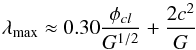 (7)where φcl is the magnetic flux per unit length and
  the thermal sound speed. The magnetic flux is here φcl = 2R0B0 = 2B0. We note that Eq. (7) differs from the Tomisaka expression due to incorporation of a factor of
  in the magnetic field and the definition of the magnetic flux per unit length. Also, the thermal pressure contribution is set to the critical value derived by Ostriker (1964)
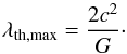 (8)For all of our models the magnetic field thus provides enough support to avoid gravitational collapse, but some of the models, that is Aa, Ab and C3a, are also thermally sub-critical as their line mass is below the critical value λth,max (see Table 2).
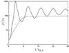 |
Fig. 1 Normalised maximum density, ρ/ρS as a function of the time for model C3b. The solid line is for the undamped evolution, while the dashed line includes drag (with C = 5). |
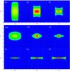 |
Fig. 2 Normalised logarithmic density, ρ/ρS, of the equilibrium configuration for the models listed in Table 1. The density range is from 0.1 to 100, except for model Ac and C3c which have a maximum density of 1000 and 300, respectively. The dashed lines show contour lines for density values of 1, 2, 3, 5, 10, 20, 30, 50, 100, 200, 300 and 500. The magnetic field lines are shown by the solid lines. |
Sub-critical filaments evolve towards their magnetohydrostatic equilibrium if no other forces are considered. We follow this evolution using the multifluid MHD code with the ambipolar resistivity set to zero, so that Eq. (5) becomes  (9)then the neutral fluid equations together with the magnetic field equation reduce to the ideal MHD equations. However, the momentum equation (see Eq. (2)) includes the Lorentz force as a source term and is thus not in its conserved form, that is
  (10)Because the momentum equation can be written in different forms, it is possible to formulate two distinct numerical approaches. An ideal MHD code uses the conserved momentum equation and one can construct a Riemann problem combining all flow variables (e.g. Brio & Wu 1988). The multifluid MHD code only solves a non-magnetic Riemann problem for the advection of the density and velocity while the magnetic field is advected separately (Falle 2003). This latter approach is simpler, but also less accurate than the former one when applied to ideal MHD. Nevertheless, the equilibrium filamentary structures calculated with both the ideal and multifluid version of MG are qualitatively identical with central densities differing only by a few percent.
The initially uniform filaments undergo gravitational contraction as there is no thermal or magnetic pressure gradient to counter self-gravity. This pressure gradient is established quickly, but the inertia of the gas causes the filaments to oscillate around their magnetohydrostatic equilibrium (see for example Fig. 1). To hasten the evolution towards the equilibrium, we damp the neutral velocity by introducing a drag force, which we decrease to zero as the simulation approaches equilibrium. This is done by adding a drag force term, that is −Cρnvn, on the left hand side of neutral momentum equation with C the drag coefficient. Figure 1 shows the temporal evolution of the central density with time for model C3b. The central density increases by nearly two orders of magnitude to its equilibrium value, that is from ρ = 0.699 to 100ρS ≈ 32 with ρS = pext/T0 the surface density of the filament within ≈5tff,S (where tff,S = (1/4πGρS)1/2 is the free-fall time evaluated with the surface density). Contrary to the undamped evolution, the filament does not oscillate as it attains it equilibrium configuration. Once the central density remains constant for several free-fall time we say the filament has reached its equilibrium configuration. The undamped solution has a higher central density that continues to increase. This is due to numerical diffusion during the contraction phase which causes the cloud to lose magnetic flux and leads to a denser filament centre than expected from its initial conditions.
Figure 2 shows the equilibrium density and magnetic field configuration for the models listed in Table 1. Comparing these structures with the analytic results of Tomisaka (2014), we find identical density and magnetic field structures and peak central densities. Models A and C3 show the effect of increasing filament mass, while models D show the effect of an increasing magnetic field strength. We also examine whether these equilibrium structures are stable. Therefore, we superimpose a turbulent velocity field with a rms sonic Mach number of 0.3 (see Sect. 5 for implementation details). We do not consider driven turbulence for this stability study. While the density structure is modified initially by the velocity perturbations, the filaments attain their original equilibrium configuration as the turbulence decays. Our results then not only confirm Tomisaka’s analytic results; they also show that the equilibria are stable.
4. Ambipolar diffusion
The magnetohydrostatic filament configurations derived in the previous section are magnetically supported against gravitational collapse. Gravitational collapse of the filament is then possible only if the line mass increases above the critical value given by Eq. (7). This can only happen if the magnetic flux decreases. In a weakly ionised plasma, ambipolar diffusion, or ion-neutral drift causes structural reorganisation of the magnetic field. When ambipolar diffusion occurs, the magnetic field diffuses out of the filament, thereby decreasing the magnetic flux. An initially magnetically sub-critical filament then becomes super-critical.
4.1. Thermally sub-critical filaments
As mentioned earlier, some of the filament models, that is Aa, Ab and C3a, are thermally sub-critical. As these filaments lose magnetic flux, their density structure is expected to evolve towards a new equilibrium state supported solely by thermal pressure gradients.
Figure 3 shows the effect of ambipolar diffusion on model C3a. Due to the gradients of the magnetic field, ambipolar diffsuion is initiated and the filament loses magnetic support against self-gravity (see panel (b)) and, consequently, the filament starts to contract (see panel (a)). As the ambipolar diffusion coefficient is inversely proportional to the fractional ionisation, the contraction rate increases with decreasing fractional ionisation. However, the contraction does not continue indefinitely. The central density only increases by a factor of approximately five, after which it remains constant and, hence, the filament reaches a new stable configuration. The magnetic flux per unit length also reaches a new stable value indicating that the magnetic field is now uniform and can no longer provide support against self-gravity. Although the filament is now magnetically super-critical, it is still thermally sub-critical. Then the filament’s density profile is given by the hydrostatic equilibrium profile (Ostriker 1964) ![Mathematical equation: \begin{equation} \label{ost} \rho(r)=\frac{\rho_0}{[1+(r/R_0)^2]^2}, \end{equation}](/articles/aa/full_html/2016/12/aa29039-16/aa29039-16-eq76.png) (11)where
(11)where  is the thermal scale height. By integrating Eq. (11) to obtain the line mass λ and taking λ = 1.718 and pext = 0.318 (see parameters for model C3a), one can show that the central density of the equilibrium cylinder needs to be ρ0 = 16.06 ≈ 50ρS. All ambipolar-diffusion regulated models attain values for ρ0 that are nearly equal to this value (see Fig. 3). As a test we also run a model with the magnetic field removed from the equilibrium configuration. This model also reproduces a similar central density, so that ambipolar diffusion clearly removes the magnetic support from the filament.
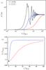 |
Fig. 3 Ambipolar diffusion regulated collapse for model C3a. The blue and red line show the evolution for X = 10-7 and X = 10-8 respectively, while the black line shows the evolution without magnetic fields. Panel a) shows the maximum (i.e. central) density, while panel b) shows the ratio of the line-mass to the critical value given by Eq. (7). The black dot shows the value for the equilibrium structure. |
Not only do we have the same central density in the simulation, model C3a can be entirely fitted with the analytic profile given by Eq. (11). Figure 4 shows the relative difference between the equilibrium density profile attained with an ambipolar diffusion model using X = 10-8 and the Ostriker density distribution with the same central density. The relative difference for most of the cylindrical filament is below 5%; the error approaches 10% only near the edge.
Similar results are obtained for the other thermally sub-critical models Aa and Ab.
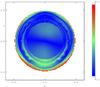 |
Fig. 4 Fractional difference between model C3a with X = 10-8 and the Ostriker hydrostatic equilibrium profile with the same central density. |
4.2. Thermally super-critical filaments
All other models are thermally super-critical and continue to collapse gravitationally until all the gas mass is in a few grid cells. Figure 5a shows the evolution of the central density for different values of X. As X decreases, the timescale for collapse also decreases, that is the collapse timescales are approximately 56.6tff,S,7tff,S and 1.71tff,S for X = 10-6,10-7 and 10-8 respectively.
This dependency can be understood by considering the flux loss timescale, tφ, for gravitational collapse. Mouschovias & Morton (1991) show that the flux loss timescale is given by 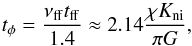 (12)where νff = tff/tni is the collapse retardation factor, tni = 1 /ρiKni the average collision time between neutrals and ions and χ the ionisation fraction at the initial time. As the fractional ionisation is given by
  , we find that the collapse time is proportional to X if the collapse time substantially exceeds the free-fall time. Using the central density of the filament for ρn, we find tφ ≈ 125tff,S for X = 10-6, ≈12.5tff,S for X = 10-7 and ≈1.25tff,S for X = 10-8. These estimated values agree within a factor of two with the numerically derived values and thus explain the near-proportional decrease in collapse timescale of the filament. However, it is clear that the proportionality needs to break down at some point as the gravitational contraction rate cannot exceed the free-fall collapse rate. Numerically the minimum collapse timescale is derived by instantaneously removing the magnetic flux support, that is setting the magnetic field values to zero and we find ≈0.9tff,S (see black line in Fig. 5). From Eq. (12), we expect this to happen when νff ≲ 1.4 or X ≲ 8 × 10⁻⁹. Bailey & Basu (2012) find a similar dependence on the ionisation fraction for the collapse time of planar sheets. A linear stability analysis shows that the collapse time for sheets with mass-to-flux ratios equivalent to our models decreases linearly until the average ion-neutral collision time becomes comparable to the free-fall collapse time of the thin sheet.
 |
Fig. 5 a) Normalised central density, ρ/ρS as a function of time for ambipolar diffusion regulated collapse of model C3b. b) Ratio of line mass to critical line mass with the black dot the value of the equilibrium profile. The squares show the ratio when the central density is 1000 ρS. The blue, red and green lines show the collapse for X = 10-8,10-7 and 10-6 respectively. The black line shows the collapse if no magnetic fields are present. |
This break is also observed in the evolution in the distribution of gas and the magnetic field in the filament. Figures 6 and 7 show the density profile and magnetic field configuration for X = 10-6,10-7 and 10-8 when the central density has a value of 250ρS and 1000ρS. (We note that these densities are attained at different times for each model.) These densities are chosen to represent an instant during the linear (250ρS) and non-linear (1000ρS) phase of the filament collapse. For X = 10-6 and 10-7, the profiles and field structure evolve identically, albeit at different collapse rates, indicating a self-similar evolution. The magnetic field for these values of X maintains its hourglass shape throughout the collapse and, during the linear phase, even preserves the field from the equilibrium distribution. Then, from Eq. (5) follows 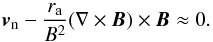 (13)As the magnetic field structure is independent of X (if X ≥ 10-7), the neutral velocity varies as ra which is inversely proportional to X (see Eq. (6)). This again explains why the collapse rate is proportional to X. The neutral speeds are small compared to the sound speed, so that the evolution is slow and much slower than the free-fall collapse, that is quasi-static. As mentioned earlier, for these values of X, νff is large. The collision timescale between neutrals and ions is therefore much shorter than the free-fall timescale, so that the neutrals are still strongly coupled to the magnetic field and the ambipolar diffusion length scale, that is λAD = πvAtni, is smaller than the Jeans’ length λJ = atff. So, the collapse of the cloud, although driven by gravity, is quasi-static and magnetically regulated. We will refer to this as gravitationally-driven magnetically-regulated ambipolar diffusion.
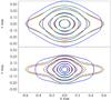 |
Fig. 6 Normalised density contours, ρ/ρS, for X = 10-8 (blue), X = 10-7 (red) and X = 10-6 (green). The top panel shows the density configuration for a central density of ≈250ρS, while the bottom shows it for ≈1000ρS. The contour line show normalised densities of 1, 3, 10, 30, 100 and 300. |
The evolution for X = 10-8 differs from the self-similar solution, although the collapse is still initiated by gravitationally-driven magnetically-regulated ambipolar diffusion. The collision timescale between neutrals and ions is not too dissimilar to the free-fall timescale. The neutrals are therefore weakly coupled to the magnetic field and the magnetic field is able to straighten itself quickly (see Fig. 7). This is particularly apparent in the outer regions of the filament where λAD>λff. We note that, in Fig. 6, the contour line for ρS = 1 is distinctly different than for the self-similar collapse. As the neutrals easily diffuse across the magnetic field lines, the neutral velocities for the collapse are much higher than before and close to the sound speed. The cloud collapse is thus a dynamical, gravity dominated process and is referred to as gravitationally-driven and -dominated ambipolar diffusion. (As both modes are gravitationally driven, we will drop the adjective gravitationally-driven for the remainder of the paper.)
Some similarities remain for both evolutionary paths, that is the density distribution in the central region of the filament is independent of the ionisation coefficient X. For the bottom panel of Fig. 6, the density distributions above ρ> 30ρS are identical. As the central region of the filament loses magnetic support, the dynamics is determined by gravity and thermal pressure gradients alone. Furthermore, the neutral velocities within the central region are much smaller than the sound speed, so that a near static equilibrium is achieved there. Within the contour of 300ρS, the relative difference between the density distribution and the Ostriker density profile (Eq. (11)) is less than 20%. So more than a third of the total line mass lies within a region accurately described by a hydrodynamical equilibrium.
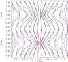 |
Fig. 7 Magnetic field lines for X = 10-8 (blue), X = 10-7 (red) and X = 10-6 (green) when the central density of the filament is ≈250ρS (top panel) and when it is ≈1000ρS (bottom panel). |
Although the filament loses magnetic support, it is important to realise that not much magnetic flux is lost from the filament due to ambipolar diffusion. Even during the non-linear collapse phase, that is when the central density reaches 1000ρS, the magnetic flux per unit length has decreased by only 5% of its initial value for X = 10-8 and less than 1% for X ≥ 10-7 (see Fig. 5b). The magnetic flux is actually redistributed within the filament. As magnetic flux is transported from the centre towards the envelope, the central regions collapse while the outer layers around the midplane remain in place. This can be seen in Fig. 6 especially for X ≥ 10-7.
While the above describes the collapse of model C3b for different ionisation coefficients, the results are generally valid for the other thermally super-critical models. Figure 8 shows the evolution of the central density and the ratio of the line mass to the critical line mass (Eq. (7)) for model D2 as the filament is collapsing. When overlaid with the evolution for model C3b renormalised in time so that the numerical time scales for the instantaneous flux loss model are the same, the trends are seen to be identical. This is expected as the collapse retardation factor only depends on the ionisation coefficient X and not on for example density. A similar argument holds for the density distribution. Again, for X ≲ 10-8 the distribution differs as the collapse is regulated by gravitationally-dominated ambipolar diffusion. For higher ionisation coefficients, magnetically-regulated ambipolar diffusion forces the filament to undergo quasi-static collapse (see Fig. 9).
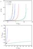 |
Fig. 8 Same figures as for Fig. 5 but for model D2. The dashed lines show the evolution for model C3b from Fig. 5 with the time renormalised so that the numerical time scale for instantaneous flux loss is the same as for model D2. |
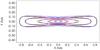 |
Fig. 9 Normalised density contours, ρ/ρS, for X = 10-8 (blue), X = 10-7 (red) and X = 10-6 (green) for model D2 when the central density is ≈200ρS. The contour line show normalised densities of 1, 3, 10, 30 and 100. |
5. Decaying turbulence and ambipolar diffusion
For high ionisation coefficients the gravitational collapse regulated by ambipolar diffusion is still a slow process compared to free-fall collapse. However, turbulence accelerates ambipolar diffusion in the absence of self-gravity (e.g. Heitsch et al. 2004; Li et al. 2012). Fatuzzo & Adams (2002) show analytically that there is an increase in the ambipolar diffusion rate, and thus the collapse rate, of a factor of a few. Three-dimensional simulations of sub-critical thin sheets further corroborate this finding as the timescale for core formation shortens when velocity perturbations are considered in addition to ambipolar diffusion (Kudoh & Basu 2011).
In order to study the effect of turbulence on the ambipolar diffusion rate, we perturbed the equilibrium distribution of model C3b by adding velocity perturbations δvx,y appropriate for turbulence to the neutral velocity. We used an approach described in Mac Low (1999), although we do not subsequently drive the turbulence. The velocity perturbations are generated by assigning an amplitude and a phase in Fourier space and transforming them back into real space. While the phase is a random number between 0 and 2π, the amplitude is drawn from a Gaussian distribution around zero and a deviation given by P(k) ∝ k-2, where k = Ld/λ is the dimensionless wave number (Ld = 2 is the largest driving wavelength). We assumed a set of wave numbers ranging from  . We also ensured that there is no net momentum input into the filament, that is ∫ρδvx,ydV = 0. Then we normalised the amplitude of the velocity perturbations so that the turbulent velocity field has a rms sonic Mach number, Mrms, of 10, 3 or 1. These values were chosen to see an effect of the turbulent motions within the filament even though the turbulence decays.
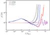 |
Fig. 10 Similar figure as Fig. 5, but with a turbulent velocity field of Mrms = 10 added to the equilibrium filament. The purple line shows the evolution of the ideal MHD filament. The dashed lines show the quiescent evolution of model C3b. |
Figure 10 shows the evolution of the maximum density in the filament as a function of time for different ionisation coefficients X and for ideal MHD with and without turbulence (the initial rms Mach number is 10). Initially the turbulent motions compress the gas locally leading to an increase in the maximum density by a factor of a few (≈2–3). However, the overall effect of the turbulence is to oppose self-gravity. Thus, the filament expands lowering the maximum density. At the same time the turbulence is decaying and, around 0.1tff,S, enough turbulent support is removed, that is Mrms reduces to ≈0.4, for the filament to collapse in the absence of magnetic fields. The turbulence significantly slows down the gravitational collapse, that is by a factor 1.6.
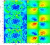 |
Fig. 11 Velocity magnitude (left) and x-component of the magnetic field (right) after 0.3tff,S for X = 10-8 (top), X = 10-7 (middle) and ideal MHD (bottom) with a initial turbulent velocity field of Mrms = 10. The contour lines show 1, 3, 10 and 30 ρS. |
The turbulence is still sufficient to support the filaments if a magnetic field is present. For magnetic-field supported filaments both magnetic support and turbulent support need to be removed. The ambipolar diffusion helps with both. As in the quiescent case ambipolar diffusion redistributes the magnetic flux within the filament so that most of the flux is in the envelope and not in the centre. The turbulent velocity field generates larger magnetic field gradients than in the quiescent case. It thus accelerates the diffusion of the magnetic field on the small scales (see right-hand term in Eq. (5)) and eventually smooths the large scale structure (Heitsch et al. 2004). At the same time, ambipolar diffusion dissipates perturbations with wavelengths below λAD (Mouschovias & Morton 1991; Van Loo et al. 2008) so that, also, turbulent support is removed. The dissipation of small-scale velocity perturbations is displayed in Fig. 11. This figure shows the magnitude of the velocity field and the x-component of the magnetic field for different ionisation coefficients at t = 0.3tff,s. At this time the models are still similar in their density profile (e.g. their central density is similar as can be seen in Fig. 10), but show variation in the velocity and magnetic field. The difference can also be quantified. While the difference in rms velocity is small when considering the entire filament (Mrms lies between 0.262 and 0.285), the rms velocity within the highest density contour (>30ρS) varies significantly between X = 10-8, X = 10-7 and ideal MHD with values of Mrms = 0.087, 0.129 and 0.148 respectively. A lower rms velocity indicates less turbulent support. The presence of the velocity perturbations is also seen in the x-component of the magnetic field. As the velocity perturbations dissipate more slowly for a higher ionisation coefficient and the gas is also more strongly coupled to the field, turbulence distorts the magnetic field to a higher degree.
Ratio of collapse time for ambipolar-diffusion regulated collapse with different ionisation coefficients to the collapse time if the magnetic field is instantaneously removed with changing levels of turbulence.
Unfortunately, it is not possible to quantify the acceleration of the ambipolar diffusion by the turbulence. The filament’s evolution depends strongly on the amount of turbulence injected and disentangling the associated effects from the ambipolar diffusion acceleration is not feasible. However, we can compare the time scale of the ambipolar-diffusion regulated collapse with the collapse time for instantaneously removal of the magnetic field to quantify the combined effect (see Table 3). The ratios for Mrms = 10 show that turbulence indeed speeds up the ambipolar diffusion process as in the simulations of Kudoh & Basu (2011). However, note from Fig. 10 that the actual time for collapse increases when turbulence is present. Turbulence adds extra support against self-gravity, but it happens both in the models with and without magnetic fields. Also, we should take into account that the ratios are only upper values as most of the turbulence decays well before the collapse is finished, especially for X = 10-7. To fully understand the interplay of ambipolar diffusion and turbulence, driven-turbulence models are needed.
6. Discussion and conclusions
In this paper we have investigated the effect of ambipolar diffusion and decaying turbulence on infinitely long, isothermal, magnetically sub-critical filaments in two dimensions. Magnetohydrostatic equilibrium filaments in pressure-equilibrium with the external medium are generated numerically in ideal MHD as initial conditions. These equilibria reproduce the analytic profiles of Tomisaka (2014) and, by perturbing the equilibria with decaying velocity perturbations, we find that these equilibrium filaments are dynamically stable.
By using a multifluid AMR MHD code, we then follow the response of the equilibrium filament to ambipolar diffusion. Due to the gradients of the magnetic field, ambipolar diffusion initiates the filament’s contraction. For thermally sub-critical filaments this contraction is halted when a new equilibrium is reached. Magnetic support is lost, with flux loss rates increasing inversely proportional to the ionisation coefficient X, but thermal pressure gradients are enough to balance gravitational forces. The new equilibrium is the hydrostatic profile described by Ostriker (1964).
For thermally super-critical filaments the filament contains enough mass to overcome thermal pressure forces and to collapse gravitationally. The collapse rate depends on the flux loss rate and is, as for the sub-critical filaments, thus inversely proportional to the ionisation coefficient X. It is important to realise that ambipolar-diffusion regulated collapse solely depends on X and no other variable such as for example density, magnetic field strength or external pressure. Two models with completely different properties, that is C3b and D2, show the same collapse times for the various values of X when normalised to the collapse time for instantaneous magnetic flux removal.
Two gravitationally-driven ambipolar diffusion regimes are observed: a magnetically-regulated one for X ≥ 10-7 and a gravitationally-dominated one for X ≲ 10-8 in agreement with Mouschovias & Morton (1991). The former arises because the collision time between neutrals and ions is much shorter than the free-fall time (or λAD<λff). Then the neutrals are strongly coupled to the magnetic field and the ambipolar diffusion is regulated by the magnetic field. The collapse is quasi-static with neutral velocities much smaller than the sound speed. In the latter regime, the ion-neutral collision time becomes comparable or longer than the free-fall time and λAD ≥ λff. The neutrals are then weakly coupled and high neutral velocites are attained.
Ambipolar-diffusion regulated collapse is a slow process compared to free-fall collapse, especially in the magnetically-regulated regime. Numerical simulations of non-gravitating clouds show that turbulence enhances ambipolar diffusion by a factor of a few (Heitsch et al. 2004; Li et al. 2012). When the equilibrium filament is perturbed by adding a decaying turbulent velocity field, we find that the ambipolar-diffusion collapse times decrease when compared to the collapse time for instantaneous magnetic flux loss. The actual time scales increase as the turbulent motions provide additional support to the filament. The effect of the turbulence on the ambipolar diffusion is to speed up the diffusion rate as larger magnetic field gradients are generated, while ambipolar diffusion dissipates the turbulence below
the ambipolar diffusion length scale. Because we only study the effect of decaying turbulence, we cannot disentangle the combined effect of turbulence and ambipolar diffusion, but the largest effect is observed for the lowest ionisation coefficient and the highest turbulent intensity.
Other effects potentially enhance the collapse rate of the magnetised filament further. In addition to ambipolar diffusion, turbulent magnetic reconnection can be an efficient diffusion process for the magnetic field (e.g. Lazarian & Vishniac 1999; Santos-Lima et al. 2010). Also, our models are restricted to 2D. Mouschovias (1991) has shown that geometry, that is the dimensionality of the problem, plays an important role in the fragmentation process due to ambipolar diffusion. In a subsequent paper we will extend these filaments to three dimensions.
Acknowledgments
We thank the anonymous referee for his/her insightful comments that have improved the paper. The calculations for this paper were performed on the DiRAC Facility jointly funded by STFC, the Large Facilities Capital Fund of BIS and the University of Leeds. C.A.B., S.A.E.G.F. and T.W.H. are supported by a STFC consolidated grant. The data presented in this paper is available at http://doi.org/10.5518/72.
References
- André, P., Men’shchikov, A., Bontemps, S., et al. 2010, A&A, 518, L102 [NASA ADS] [CrossRef] [EDP Sciences] [Google Scholar]
- Bailey, N. D., & Basu, S. 2012, ApJ, 761, 67 [NASA ADS] [CrossRef] [Google Scholar]
- Bonnell, I. A., Dobbs, C. L., Robitaille, T. P., & Pringle, J. E. 2006, MNRAS, 365, 37 [NASA ADS] [CrossRef] [Google Scholar]
- Brio, M., & Wu, C. C. 1988, J. Comput. Phys., 75, 400 [NASA ADS] [CrossRef] [Google Scholar]
- Dedner, A., Kemm, F., Kröner, D., et al. 2002, J. Comput. Phys., 175, 645 [Google Scholar]
- Elmegreen, B. G. 1979, ApJ, 231, 372 [NASA ADS] [CrossRef] [Google Scholar]
- Engargiola, G., Plambeck, R. L., Rosolowsky, E., & Blitz, L. 2003, ApJS, 149, 343 [NASA ADS] [CrossRef] [Google Scholar]
- Falle, S. A. E. G. 2003, MNRAS, 344, 1210 [NASA ADS] [CrossRef] [Google Scholar]
- Fatuzzo, M., & Adams, F. C. 2002, ApJ, 570, 210 [NASA ADS] [CrossRef] [Google Scholar]
- Heitsch, F., Zweibel, E. G., Slyz, A. D., & Devriendt, J. E. G. 2004, ApJ, 603, 165 [NASA ADS] [CrossRef] [Google Scholar]
- Kudoh, T., & Basu, S. 2011, ApJ, 728, 123 [NASA ADS] [CrossRef] [Google Scholar]
- Kudoh, T., & Basu, S. 2014, ApJ, 794, 127 [NASA ADS] [CrossRef] [Google Scholar]
- Kudoh, T., Basu, S., Ogata, Y., & Yabe, T. 2007, MNRAS, 380, 499 [NASA ADS] [CrossRef] [Google Scholar]
- Lazarian, A., & Vishniac, E. T. 1999, ApJ, 517, 700 [NASA ADS] [CrossRef] [Google Scholar]
- Li, P. S., McKee, C. F., & Klein, R. I. 2012, ApJ, 744, 73 [NASA ADS] [CrossRef] [Google Scholar]
- Li, H.-B., Fang, M., Henning, T., & Kainulainen, J. 2013, MNRAS, 436, 3707 [NASA ADS] [CrossRef] [Google Scholar]
- Mac Low, M.-M. 1999, ApJ, 524, 169 [NASA ADS] [CrossRef] [Google Scholar]
- McKee, C. F., & Zweibel, E. G. 1995, ApJ, 440, 686 [NASA ADS] [CrossRef] [Google Scholar]
- Mestel, L., & Spitzer, L., Jr. 1956, MNRAS, 116, 503 [NASA ADS] [CrossRef] [Google Scholar]
- Mouschovias, T. C. 1976, ApJ, 207, 141 [NASA ADS] [CrossRef] [Google Scholar]
- Mouschovias, T. C. 1979, ApJ, 228, 475 [NASA ADS] [CrossRef] [Google Scholar]
- Mouschovias, T. C. 1991, ApJ, 373, 169 [NASA ADS] [CrossRef] [Google Scholar]
- Mouschovias, T. C., & Morton, S. A. 1991, ApJ, 371, 296 [NASA ADS] [CrossRef] [Google Scholar]
- Ostriker, J. 1964, ApJ, 140, 1056 [NASA ADS] [CrossRef] [MathSciNet] [Google Scholar]
- Sakamoto, S., Hayashi, M., Hasegawa, T., Handa, T., & Oka, T. 1994, ApJ, 425, 641 [NASA ADS] [CrossRef] [Google Scholar]
- Santos-Lima, R., Lazarian, A., de Gouveia Dal Pino, E. M., & Cho, J. 2010, ApJ, 714, 442 [NASA ADS] [CrossRef] [Google Scholar]
- Takahira, K., Tasker, E. J., & Habe, A. 2014, ApJ, 792, 63 [NASA ADS] [CrossRef] [Google Scholar]
- Tomisaka, K. 2014, ApJ, 785, 24 [NASA ADS] [CrossRef] [Google Scholar]
- Truelove, J. K., Klein, R. I., McKee, C. F., et al. 1997, ApJ, 489, L179 [NASA ADS] [CrossRef] [Google Scholar]
- Vaidya, B., Hartquist, T. W., & Falle, S. A. E. G. 2013, MNRAS, 433, 1258 [NASA ADS] [CrossRef] [Google Scholar]
- Van Loo, S., Falle, S. A. E. G., & Hartquist, T. W. 2007, MNRAS, 376, 779 [NASA ADS] [CrossRef] [Google Scholar]
- Van Loo, S., Falle, S. A. E. G., Hartquist, T. W., & Barker, A. J. 2008, A&A, 484, 275 [NASA ADS] [CrossRef] [EDP Sciences] [Google Scholar]
- Van Loo, S., Keto, E., & Zhang, Q. 2014, ApJ, 789, 37 [NASA ADS] [CrossRef] [Google Scholar]
- Vázquez-Semadeni, E., Banerjee, R., Gómez, G. C., et al. 2011, MNRAS, 414, 2511 [NASA ADS] [CrossRef] [Google Scholar]
All Tables
Initial conditions given in dimensionless units along with the resolution of each model and the name of the corresponding Tomisaka model.
Ratio of collapse time for ambipolar-diffusion regulated collapse with different ionisation coefficients to the collapse time if the magnetic field is instantaneously removed with changing levels of turbulence.
All Figures
|
Fig. 1 Normalised maximum density, ρ/ρS as a function of the time for model C3b. The solid line is for the undamped evolution, while the dashed line includes drag (with C = 5). |
| In the text | |
|
Fig. 2 Normalised logarithmic density, ρ/ρS, of the equilibrium configuration for the models listed in Table 1. The density range is from 0.1 to 100, except for model Ac and C3c which have a maximum density of 1000 and 300, respectively. The dashed lines show contour lines for density values of 1, 2, 3, 5, 10, 20, 30, 50, 100, 200, 300 and 500. The magnetic field lines are shown by the solid lines. |
| In the text | |
|
Fig. 3 Ambipolar diffusion regulated collapse for model C3a. The blue and red line show the evolution for X = 10-7 and X = 10-8 respectively, while the black line shows the evolution without magnetic fields. Panel a) shows the maximum (i.e. central) density, while panel b) shows the ratio of the line-mass to the critical value given by Eq. (7). The black dot shows the value for the equilibrium structure. |
| In the text | |
|
Fig. 4 Fractional difference between model C3a with X = 10-8 and the Ostriker hydrostatic equilibrium profile with the same central density. |
| In the text | |
|
Fig. 5 a) Normalised central density, ρ/ρS as a function of time for ambipolar diffusion regulated collapse of model C3b. b) Ratio of line mass to critical line mass with the black dot the value of the equilibrium profile. The squares show the ratio when the central density is 1000 ρS. The blue, red and green lines show the collapse for X = 10-8,10-7 and 10-6 respectively. The black line shows the collapse if no magnetic fields are present. |
| In the text | |
|
Fig. 6 Normalised density contours, ρ/ρS, for X = 10-8 (blue), X = 10-7 (red) and X = 10-6 (green). The top panel shows the density configuration for a central density of ≈250ρS, while the bottom shows it for ≈1000ρS. The contour line show normalised densities of 1, 3, 10, 30, 100 and 300. |
| In the text | |
|
Fig. 7 Magnetic field lines for X = 10-8 (blue), X = 10-7 (red) and X = 10-6 (green) when the central density of the filament is ≈250ρS (top panel) and when it is ≈1000ρS (bottom panel). |
| In the text | |
|
Fig. 8 Same figures as for Fig. 5 but for model D2. The dashed lines show the evolution for model C3b from Fig. 5 with the time renormalised so that the numerical time scale for instantaneous flux loss is the same as for model D2. |
| In the text | |
|
Fig. 9 Normalised density contours, ρ/ρS, for X = 10-8 (blue), X = 10-7 (red) and X = 10-6 (green) for model D2 when the central density is ≈200ρS. The contour line show normalised densities of 1, 3, 10, 30 and 100. |
| In the text | |
|
Fig. 10 Similar figure as Fig. 5, but with a turbulent velocity field of Mrms = 10 added to the equilibrium filament. The purple line shows the evolution of the ideal MHD filament. The dashed lines show the quiescent evolution of model C3b. |
| In the text | |
|
Fig. 11 Velocity magnitude (left) and x-component of the magnetic field (right) after 0.3tff,S for X = 10-8 (top), X = 10-7 (middle) and ideal MHD (bottom) with a initial turbulent velocity field of Mrms = 10. The contour lines show 1, 3, 10 and 30 ρS. |
| In the text | |
Current usage metrics show cumulative count of Article Views (full-text article views including HTML views, PDF and ePub downloads, according to the available data) and Abstracts Views on Vision4Press platform.
Data correspond to usage on the plateform after 2015. The current usage metrics is available 48-96 hours after online publication and is updated daily on week days.
Initial download of the metrics may take a while.