| Issue |
A&A
Volume 596, December 2016
|
|
|---|---|---|
| Article Number | A31 | |
| Number of page(s) | 12 | |
| Section | Stellar structure and evolution | |
| DOI | https://doi.org/10.1051/0004-6361/201628583 | |
| Published online | 25 November 2016 | |
Photospheric and chromospheric magnetic activity of seismic solar analogs
Observational inputs on the solar-stellar connection from Kepler and Hermes ⋆
1 Laboratoire AIM, CEA/DRF-CNRS, Université Paris 7 Diderot, IRFU/SAp, Centre de Saclay, 91191 Gif-sur-Yvette, France
e-mail: david.salabert@cea.fr
2 High Altitude Observatory, National Center for Atmospheric Research, PO Box 3000, Boulder, CO 80307-3000, USA
3 Department of Physics, Montana State University, Bozeman, MT 59717-3840, USA
4 Instituto de Astrofísica de Canarias, 38200 La Laguna, Tenerife, Spain
5 Departamento de Astrofísica, Universidad de La Laguna, 38205 La Laguna, Tenerife, Spain
6 Space Science Institute, 4750 Walnut street Suite#205, Boulder, CO 80301, USA
7 Visiting Scientist, National Solar Observatory, 3665 Discovery Dr., Boulder, CO 80303, USA
8 Universidade Federal do Rio Grande do Norte, UFRN, Dep. de Física, DFTE, CP1641, 59072-970 Natal, RN, Brazil
9 Harvard-Smithsonian Center for Astrophysics, Cambridge, MA 02138, USA
10 Stellar Astrophysics Centre, Department of Physics and Astronomy, Aarhus University, Ny Munkegade 120, 8000 Aarhus C, Denmark
Received: 23 March 2016
Accepted: 3 August 2016
We identify a set of 18 solar analogs among the seismic sample of solar-like stars observed by the Kepler satellite rotating between 10 and 40 days. This set is constructed using the asteroseismic stellar properties derived using either the global oscillation properties or the individual acoustic frequencies. We measure the magnetic activity properties of these stars using observations collected by the photometric Kepler satellite and by the ground-based, high-resolution Hermes spectrograph mounted on the Mercator telescope. The photospheric (Sph) and chromospheric ( index) magnetic activity levels of these seismic solar analogs are estimated and compared in relation to the solar activity. We show that the activity of the Sun is comparable to the activity of the seismic solar analogs, within the maximum-to-minimum temporal variations of the 11-yr solar activity cycle 23. In agreement with previous studies, the youngest stars and fastest rotators in our sample are actually the most active. The activity of stars older than the Sun seems to not evolve much with age. Furthermore, the comparison of the photospheric, Sph, with the well-established chromospheric, index, indicates that the Sph index can be used to provide a suitable magnetic activity proxy which can be easily estimated for a large number of stars from space photometric observations.
Key words: stars: solar-type / stars: activity / stars: evolution / methods: data analysis / methods: observational
© ESO, 2016
1. Introduction
The Sun is a G-type star with a quasi-periodic 11-yr magnetic activity cycle that is most apparent in the rise and fall of the occurrence of small regions of strong magnetic field which appear as dark spots on the surface in the visible wavelengths (Hathaway 2015, and references therein). This behavior is believed to be the result of an internal dynamo process driven by the rotational and convective motions of the plasma in the outer convective layers of the star (Charbonneau 2010, and references therein). Numerous physical models have been proposed to govern the amplification and reconfiguration of global-scale toroidal and poloidal field components in the observed cyclic fashion, yet as of today no ab initio physical model exists which can explain all of the variety of behavior in the sunspot cycle, and parameterized and empirical models do not yet reliably predict basic features such as cycle amplitudes or durations (Petrovay 2010, and references therein).
The question of whether variable magnetic activity occurs in other stars was answered in the affirmative using long-term synoptic observations of the Ca ii H and K lines. Over decades, extensive observational projects at Mount Wilson Observatory (MWO; Wilson 1978; Duncan et al. 1991) and at Lowell Observatory (Hall et al. 2007) were dedicated to measure the strength and the modulation of plasma emissions in the stellar chromosphere. These emissions, resulting from the non-thermal heating that occurs in the presence of strong magnetic fields, are quantified through the so-called (Wilson 1978) and  (Noyes et al. 1984) indices. They strongly correlate with the presence of solar plage areas surrounding active regions, and thereby make for excellent proxies of magnetic activity (Keil & Worden 1984).
With stellar data on magnetic activity, it then became possible to study the operation of dynamos in objects with different fundamental properties, such as mass and rotation rate. The MWO Ca ii H and K data were used to explore the relationship between magnetic activity and rotation, and it was found that stars that rotate faster have higher magnetic activity (Vaughan et al. 1981; Baliunas et al. 1983; Noyes et al. 1984). In addition, it was observed that activity decreases with stellar ages (Skumanich 1972; Soderblom et al. 1991). Activity is also sensitive to stellar mass. Indeed, for stars with similar rotation the less massive stars tend to have higher activity (Noyes et al. 1984). Baliunas et al. (1995) reported the results of 25 yr of MWO observations for a set of 111 lower main-sequence stars which revealed a range of long-term variable behavior, from solar-like and shorter cycles, to flat-activity and irregular variables. Saar & Baliunas (1992) and Soon et al. (1993) reported two distinct branches of cycling stars, the active and inactive branches with respectively a higher and lower number of rotations per cycle. Brandenburg et al. (1998) and Saar & Brandenburg (1999) studied these dynamo branches with a larger sample of stars in terms of dimensionless quantities relevant to mean-field dynamo theory, and Böhm-Vitense (2007) observes that the Sun lies squarely between the two branches in a high-quality subset of the same sample, thus appearing as a peculiar outlier among the cycling stars. In addition, Lockwood et al. (2007) compared the photospheric variability in the visible Strömgren b and y bands to the magnetic activity, and find the Sun to be near the border in activity by which stars are either spot-dominated and have visible emission anti-correlated with magnetic activity, and those which are faculae-dominated and have a positive correlation. Whether the solar dynamo and the related surface magnetic activity are typical or peculiar remains an open question which can only be answered by the careful study of solar-analog stars. The answer to this question is relevant to dynamo theory, which may have more difficulty explaining the behavior of an outlier.
Finding solar-analog stars with fundamental properties as close as possible to the Sun (Cayrel de Strobel 1996) and studying the characteristics of their surface magnetic activity is a very promising way to understand the solar variability and its associated dynamo processes. Moreover, a more detailed knowledge of the magnetic activity of solar analogs is also important for understanding the evolution of the Sun and its environment in relation to other stars and the habitability of planets. Nevertheless, the identification of solar-analog stars depends on the accuracy of the estimated fundamental stellar parameters. The unprecedented quality of the continuous four-year photometric observations collected by the Kepler satellite (Borucki et al. 2010) allowed the measurements of acoustic oscillations in hundreds of solar-like stars (Chaplin et al. 2014). Indeed, the addition of asteroseismic data was proven to provide the most accurate fundamental properties that can be derived from stellar modeling today, either from global oscillation properties (Chaplin et al. 2014) or from fit individual frequencies (Mathur et al. 2012; Metcalfe et al. 2014), compared to empirical scaling-law relations (Kjeldsen & Bedding 1995). In the near future, even tighter constraints on stellar parameters will be met with the use of the astrometric observations collected by the Gaia satellite (Perryman et al. 2001).
Furthermore, the knowledge of the stellar rotation period is a key parameter in order to explain stellar activity (Brun et al. 2015, and references therein). The passage of spots of different sizes at different latitudes as the star rotates induces a modulation in its luminosity which is used to infer the rotation period of the stars. The measurements of thousands of stellar rotation periods of main-sequence stars (Nielsen et al. 2013; Reinhold & Reiners 2013; McQuillan et al. 2013, 2014) were obtained from the Kepler observations. Accurate periods of surface rotation were also measured for 310 (García et al. 2014) of the 540 pulsating solar-like field Kepler stars (Chaplin et al. 2014) and for 11 (Ceillier et al. 2016) of the 27 exoplanet-host stars (Kepler Objects of Interest, KOI) modeled by Silva Aguirre et al. (2015) using asteroseismic measurements. A detailed comparison between the different methods developed to extract the surface rotation can be found in Aigrain et al. (2015).
Based on the rotation period of the star, Mathur et al. (2014a) defined a photospheric proxy of stellar magnetic variability, called Sph, derived from the analysis of the light-curve fluctuations. Its calculation was adapted from the starspot proxy proposed by García et al. (2010) where they show that the photometric proxy of the F-type HD 49933 observed by the Convection, Rotation, and planetary Transits (CoRoT; Baglin et al. 2006) satellite is correlated with its magnetic activity. As the variability in the light curves can have different origins and timescales (magnetic activity, convection, oscillations, companion), the rotation period needs to be taken into account when calculating a photometric magnetic proxy. The photospheric surface proxy Sph can be thus used to estimate the magnetic activity of the Kepler (Mathur et al. 2014b; García et al. 2014; Salabert et al. 2016) and CoRoT (Ferreira Lopes et al. 2015) targets, where, for instance, spectral observations used to derive established activity proxies (as the and indices) do not exist and are difficult to obtain for a large number of faint stars. Other photospheric metrics were developed to study the stellar variability in the Kepler data but they do not use the knowledge of the rotation rate in their definition (Basri et al. 2010, 2011; Chaplin et al. 2011; Campante et al. 2014).
In addition, Salabert et al. (in prep.) measured the Sph index for the Sun using observations from the Variability of Solar Irradiance and Gravity Oscillations (VIRGO; Fröhlich et al. 1995) instrument onboard the Solar and Heliospheric Observatory (SoHO; Domingo et al. 1995) spacecraft. The VIRGO instrument is composed of three Sun photometers (SPM) at 402 nm (the blue channel), 500 nm (the green channel), and 862 nm (the red channel). The activity index of the Sun thus derived is shown to be very well correlated with common solar surface activity proxies, such as, among others, the sunspot number, the 10.7-cm radio flux, and the chromospheric Ca K line emission. Such photospheric proxy can be thus used to compare the magnetic activity of the Sun to solar-analog stars observed by Kepler.
In this work, we identify a set of solar analogs as defined in Sect. 2 and observed by the Kepler satellite among the seismic sample of solar-like stars from Chaplin et al. (2014). This set is constructed using the asteroseismic stellar properties found in the literature and derived using either the global oscillation properties (Chaplin et al. 2014) and the individual acoustic frequencies (Mathur et al. 2012; Metcalfe et al. 2014), and for which a surface rotation period was measured (García et al. 2014). In Sect. 3, we describe the set of observations collected by the photometric Kepler satellite and by the spectroscopic Hermes instrument (Raskin et al. 2011; Raskin 2011) used in this analysis to measure the magnetic activity properties of these stars. In Sects. 4 and 5, we respectively estimate the photospheric (Sph) and chromospheric ( index) magnetic activity levels of these seismic solar analogs, and compare them in relation to the observed solar magnetic activity. We discuss the results in Sect. 6 and conclude in Sect. 7.
References of the initial Kepler sample of seismic solar-like stars with measured stellar rotation and the identified seismic solar analogs.
2. Defining the sample of seismic solar analogs
Cayrel de Strobel (1996) provided a definition of a solar analog based on the fundamental parameters of the star such as the mass and the effective temperature. However, any definition depends on the accuracy of the measured properties and their intrinsic importance in the characterization of a solar analog. Today, asteroseismology combined with high-resolution spectroscopy has allowed to substantially improve the accuracy of the stellar parameters and to reduce their errors (Mathur et al. 2012; Chaplin et al. 2014; Metcalfe et al. 2014). Furthermore, Chaplin et al. (2011) show evidences that the magnetic activity inhibits the amplitudes of solar-like oscillations. Indeed, in the case of the Sun, the amplitudes of the acoustic modes decrease by about 15% between solar minimum and maximum for the low-degree modes (see e.g., Salabert et al. 2003, and references therein), which are the modes detectable in observations of solar-like stars. In consequence, the selection of stars analog to the Sun should include the detection of solar-like oscillations as an additional selection criterium. This is what we called a seismic solar-analog star, thus extending the Cayrel de Strobel (1996)’s definition.
In this work, we also took into account the typical observational asteroseismic, photometric, and spectroscopic uncertainties returned on the derived stellar parameters. The mass, M, has indeed to be within ±10% of the solar mass to which we added 5% which corresponds to the mean errors on the seismic masses derived using individual oscillation frequencies (Metcalfe et al. 2014). The effective temperature, Teff, has to be within ±150 K to the solar effective temperature, to which we account for a typical error of 100 K (Bruntt et al. 2012). The surface gravity, log g, must be within ±0.3 dex of the solar value. The selection was thus based on the following: (1) 0.85 M⊙ ≤ M ≤ 1.15 M⊙; (2) 5520 K ≤ Teff ≤ 6030 K; and (3) 4.14 ≤ log g ≤ 4.74. Moreover, we included in the sample only the stars with a measured rotation period (García et al. 2014) to ensure the presence of magnetic activity. In addition, we limited also the selection to stars with a large frequency separation Δν ≥ 85 μHz in order to avoid evolved stars. For comparison, Δν⊙ ≃ 135 μHz for the Sun (e.g., Grec et al. 1980). The values of Δν were taken from Chaplin et al. (2014) which were estimated from one month each of the short-cadence (SC) Kepler survey mode. Nonetheless, we checked that consistent values within the error bars were obtained when analyzing the entire SC data collected over the ~4 yr of the Kepler mission using the A2Z pipeline (Mathur et al. 2010). We note also that the solar values were taken to be: Teff = 5777 K and log g = 4.44.
Seismic solar analogs observed by Kepler and their derived stellar properties.
A total of 18 seismic solar analogs were then identified from the photometric Kepler observations of the solar-like oscillators (Chaplin et al. 2014). To do so, we chose the stellar parameters estimated using the individual frequencies whenever available, because they were derived with a better precision (Metcalfe et al. 2014). Otherwise we used the results obtained from the analysis of the global oscillation properties. Among these 18 stars, the stellar parameters of five of them were derived with the Asteroseismic Modeling Portal (AMP; Metcalfe et al. 2009) using individual frequencies and spectroscopy (Mathur et al. 2012; Metcalfe et al. 2014). The remaining 13 seismic solar analogs were identified through the stellar parameters derived using grid modeling of the global oscillation properties (Chaplin et al. 2014), for 11 of them combined with the atmospheric properties from the SDSS photometric survey (Pinsonneault et al. 2012), and for two of them with the spectroscopic properties obtained with ESPaDOnS and NARVAL observations (Bruntt et al. 2012). However, the accuracy on the associated stellar parameters derived with photometry is less than for the ones estimated using spectroscopic analysis.
Table 1 summarizes the different literature sources of the stellar parameters of the oscillating solar-like stars used in the initial sample and the associated numbers of identified seismic solar analogs with measured surface rotation, while their corresponding KIC numbers and stellar properties are given in Table 2. The references of the derived stellar parameters used in this work are provided by the column “Ref.”: (1) when global oscillation properties and photometry were used (Chaplin et al. 2014); (2) when global oscillation properties and spectroscopy were used (Chaplin et al. 2014); (3) and (4) when individual acoustic frequencies and spectroscopy were used, respectively in Mathur et al. (2012) and Metcalfe et al. (2014). Finally, some seismic solar analogs were identified in more than one literature source, as indicated in the column “Sources”. In that case, we favored the stellar parameters estimated with a known better accuracy, whose reference is given in the column “Ref.”. We note also that all the 18 seismic solar analogs identified in this work from the Kepler sample rotate between 10 and 40 days, with only seven stars rotating faster than 20 days. Finally, the crowding factor of the selected stars was checked to be less than 1%, which implies almost no risk of pollution by nearby field stars.
We also note that two of these stars were studied with greater details. A comprehensive differential analysis of Hermes spectroscopic observations of KIC 3241581, with seismic properties similar to the Sun, was performed by Beck et al. (2015), revealing that this is actually a binary system. Both the photospheric activity and the p-mode oscillation frequencies of the young (1 Gyr-old) solar analog KIC 10644253 are shown to vary with a temporal modulation of about 1.5 yr (Salabert et al. 2016). In addition, two stars, KIC 7296438 and KIC 11127479, are reported as candidates for hosting a planetary system in the KOI list.
3. Observations
3.1. Photometric observations from the Kepler satellite
The long-cadence (LC) observations of temporal sampling of 29.4244 min collected by the Kepler satellite over almost the entire duration of the mission from 2009 June 20 (Quarter 2, hereafter Q2) to 2013 May 11 (Q17; i.e., a total of 1422 days) were used in this analysis. The two first quarters Q0 (~10 days) and Q1 (~33 days) were dropped because of calibration problems since it is performed quarter by quarter. All the light curves were corrected for instrumental problems using the Kepler Asteroseismic Data Analysis and Calibration Software (KADACS, García et al. 2011). The time series were then high-pass filtered in a quarter by quarter basis using a triangular smooth function with a cut off of 55 days (see Appendix A regarding the choice of the filter). The signature of photospheric magnetic activity can be thus inferred by studying the temporal fluctuations of the light curves.
3.2. Spectroscopic observations from the HERMES instrument
Complementary high-resolution spectroscopic observations (R = 85 000) of the 18 identified seismic solar analogs were obtained with the Hermes spectrograph, mounted to the 1.2-m Mercator telescope at the Observatorio del Roque de los Muchachos (La Palma, Canary Islands, Spain). For 16 of the stars, the Hermes observations were performed over two observing runs of three days each in June and July 2015, covering a temporal interval, ΔT, of about 35 days. The 2 other targets, KIC 3241581 and KIC 10644253, were put on a long-term monitoring program with the Hermes spectrograph and thus longer temporal coverages are available (Beck et al. 2015; Salabert et al. 2016). Observations between April 2014 and September 2015 (ΔT = 504 days) and between March 2015 and September 2015 (ΔT = 180 days) were respectively used in this analysis. Details are provided in Table 3. The data reduction of the raw observations was performed with the instrument-specific pipeline (Raskin et al. 2011). The covered wavelength range is between 375 and 900 nm. The radial velocity, RV, was measured for each individual spectrum with a cross-correlation analysis using the G2-mask in the Hermes pipeline toolbox. See Beck et al. (2015) for more details regarding the data processing of the Hermes observations.
Photospheric and chromospheric activity properties of the 18 seismic solar analogs derived from the photometric Kepler and spectroscopic Hermes observations.
Binary systems discovered with the Hermes spectroscopic observations within the sample of seismic solar analogs.
Given the sparse sampling and the limited period of time, only stars with a maximum difference in radial velocity, ΔRV, of more than 1 km s-1 are considered as binary candidates. Besides the confirmed binary KIC 3241581 (Beck et al. 2015), three additional stars exceed this limit: KIC 4914923, KIC 7296438, and KIC 9098294 (see Table 4). The KIC 7296438 and KIC 9098294 systems are however the most noticeable with a ΔRV of 16.57 km s-1 and of 41.35 km s-1 respectively. Moreover, none of these three systems shows eclipses or tidally induced flux modulation in their light curve. We also note that the system KIC 7296438 is listed as a planetary host candidate (see Table 2). However, the detected variation in RV is only compatible with a stellar binary and not with a companion of substellar mass. Moreover, the spectroscopic data suggest that there could be other long periodic binary systems in our sample but they are close to our current significance threshold. Therefore, more data are needed to verify the binary nature of those systems (Beck et al., in prep.). Nonetheless, we found that the magnetic activity of the detected binaries do not differ from the one derived for single field stars (see Table 3). A detailed discussion of the observation of binary stars with solar-like oscillating primaries detected with the Hermes spectrograph can be found in Beck et al. (2014).
4. Photospheric magnetic activity
4.1. The Sph proxy
The photospheric activity proxy, Sph, is a measurement of stellar magnetic variability derived by means of the surface rotation, Prot (Mathur et al. 2014b; García et al. 2014; Ferreira Lopes et al. 2015; Salabert et al. 2016). We recall that the surface rotation can be inferred through the periodic luminosity fluctuations induced by the passage of spots in the line of sight (see e.g., Nielsen et al. 2013; Reinhold & Reiners 2013; McQuillan et al. 2013, 2014; García et al. 2014). The Sph proxy is defined as the mean value of the light curve fluctuations estimated as the standard deviations calculated over subseries of length 5 × Prot. In this way, Mathur et al. (2014a) demonstrate that most of the measured variability is only related to the magnetism (i.e., the spots) and not to the other sources of variability at different timescales, such as convective motions, oscillations, stellar companion, or instrumental problems. However, we note that such proxy represents a lower limit of the stellar photospheric activity because it depends on the inclination angle of the rotation axis in relation to the line of sight. This is also assuming that the development of the latitudinal distribution of the starspots is comparable to the one observed for the Sun, that is from mid to low latitudes, which would underestimate the Sph for highly inclined stars. Finally, the error on Sph was returned as the standard error of the mean value.
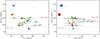 |
Fig. 1 Left panel: photospheric magnetic activity index, Sph (in ppm), as a function of the rotational period, Prot (in days), of the 18 seismic solar analogs observed with the Kepler satellite. The mean activity level of the Sun calculated from the VIRGO/SPM observations is represented for a rotation of 25 days with its astronomical symbol, and its mean activity levels at minimum and maximum of the 11-yr cycle are represented by the horizontal dashed lines. Right panel: same as the left panel but as a function of the seismic age (in Gyr). The position of the Sun is also indicated for an age of 4.567 Gyr. The size of the symbols is inversely proportional to the rotation period, Prot. In both panels, each star is referred by the same number as given in Tables 2 and 3. |
4.2. Relation with rotation and age
The values of the photospheric activity proxy, Sph, of the 18 seismic solar analogs were then measured over 1422 days of Kepler observations. We used here the rotation periods, Prot, estimated by García et al. (2014). The magnitude correction of the photon noise provided by Jenkins et al. (2010) was then applied to the Sph for each of the analyzed star. The measured Sph are given in Table 3, which summarizes the results of the magnetic activity properties of these stars. The left panel of Fig. 1 shows on a y-log scale the photospheric magnetic activity levels, Sph, of the 18 seismic solar analogs as a function of their rotational periods, Prot. The color and symbol codes correspond to the different sources of observations used to derive the stellar parameters, as described in Table 2: (1) green upside down triangles: global oscillation properties and photometry (Chaplin et al. 2014); (2) blue squares: global oscillation properties and spectroscopy (Chaplin et al. 2014); (3) orange triangles: one-month individual acoustic frequencies and spectroscopy (Mathur et al. 2012); and (4) red dots: nine-month individual acoustic frequencies fit by Appourchaux et al. (2012) and spectroscopy (Metcalfe et al. 2014).
The mean value of the photospheric activity level of the Sun, Sph, Cycle 23 ⊙ = 189.9 ± 0.5 ppm, calculated from the observations collected by the VIRGO/SPM photometers covering the entire cycle 23 (1996–2008) for a equatorial rotation Prot, ⊙ = 25 days is also indicated (Salabert et al., in prep.). We only used data covering cycle 23, because during the unusually deep and extended activity minimum of cycle 24, the Sun reached activity values considerably lower than in any of its previously observed minima (see Hathaway 2015, and references therein). In order to monitor the long-lived features on the solar surface, the VIRGO/SPM data were processed through the KADACS pipeline as described in Sect. 3.1. A composite photometric time series obtained by combining the observations from the green and red channels was used. Indeed, the Kepler broad bandpass includes these two channels at 500 and 862 nm respectively (Basri et al. 2010). In addition, the horizontal lines correspond to the photospheric magnetic activity levels of the Sun estimated at minimum and maximum of cycle 23, respectively Sph,Min23 ⊙ = 67.4 ± 0.2 ppm and Sph,Max24 ⊙ = 314.5 ± 0.8 ppm. These values were reported in Fig. 1.
The photospheric activity level of the identified seismic solar analogs falls for most of them (15 out of 18) within the range of activity covered between the minimum and the maximum of the solar cycle. Two stars with a rotation period of about 10 days are more active than the Sun at its maximum: KIC 5774694 and KIC 10644253 with respective magnetic photospheric activity of 8 × Sph,Max ⊙ and 2 × Sph,Max ⊙. Only one analog, KIC 7680114, with a rotation period comparable to the Sun, is observed to have a photospheric activity slightly lower than the Sun at its minimum of the magnetic cycle by about 0.7 × Sph,Min ⊙.
The right panel of Fig. 1 shows for the same set of 18 stars the measured photospheric activity levels, Sph, as a function of their seismic ages (taken from Mathur et al. 2012; Chaplin et al. 2014; Metcalfe et al. 2014, and reported in Table 2) compared to the Sun. The color code is the same as in the left panel of Fig. 1 but the size of the symbols is inversely proportional to the surface rotation period, Prot. We note the large differences in the uncertainties of the age estimates depending on the applied method to derive them (see Metcalfe et al. 2014). It is also worth noticing that stars between 2 and 5 Gyr-old are missing in our sample. Nevertheless, the position of the Sun indicates that its photospheric activity is compatible with older solar analogs. Although the Kepler seismic sample contains only few stars younger than the Sun (Mathur et al. 2012; Chaplin et al. 2014; Metcalfe et al. 2014), our results show that the two youngest seismic solar analogs in our sample below 2 Gyr-old are actually the most active, as well as being the fastest rotating stars as mentioned above: KIC 5774694 and KIC 10644253. Furthermore, the photospheric activity of stars older than the Sun seems to not evolve much with age. Pace (2013) studied the chromospheric activity of field dwarf stars as an age indicator, and shows that it stops decaying for stars older than 2 Gyr-old. The photospheric activity of the solar analogs analyzed in this work is observed to be comparable to the Sun after 2 Gyr-old within the minimum-to-maximum range of the solar cycle, given the uncertainties on the age estimates and the limited size of our sample. This is also assuming that our sample is not too biased towards stars observed during periods of low activity of their magnetic cycles, or that they are not in an extended cycle. Nevertheless, observations of additional solar analogs younger than the Sun are needed to fill the range of ages below 5 Gyr-old.
4.3. Dependence on the inclination angle
In the case of the Sun, spots are preferably formed between ±55° of latitude and appear closer and closer to the equator as the cycle progresses. This temporal and latitudinal development of sunspots is illustrated by the so-called butterfly diagram. In solar-like stars, preliminary observations of the spatial distribution of magnetic fields are accessible with spectropolarimetric data (see e.g., Alvarado-Gómez et al. 2015; Folsom et al. 2016, and references therein). Nevertheless, in photometric observations, the signature of temporal magnetic fluctuations is dependent on the line of sight in relation to the inclination angle of the rotation axis of the star. The estimation of the inclination angle requires three independent observables: the projected rotational velocity, υ sin i, the rotation period, Prot, and the model-dependent radius, R. These three parameters are measured with intrinsic and different accuracy with varying associated uncertainties. This thus makes difficult to have accurate estimates of the inclination of the rotation axis with satisfactory error bars in order to be able to calibrate the photospheric proxy, Sph, with the angle. Bruntt et al. (2012) and Molenda-Żakowicz et al. (2013) provided υ sin i values measured from spectroscopic observations for some of our Kepler sample of seismic solar analogs, but unfortunately with large uncertainties. Asteroseismic estimates of υ sin i were also obtained by Doyle et al. (2014) through the peak-fitting analysis of the oscillation modes for some of the stars studied here. Moreover, more accurate estimates of the asteroseismic υ sin i will be derived for fast rotators as the rotational splittings between the mode components will be larger, while for slow rotators like the Sun, it is very challenging to determine (Ballot et al. 2008).
Most of the stars in our Kepler sample of solar analogs can be considered as slow rotators. Only three stars spin in less than 15 days. In the case of KIC 10644253, the fastest rotator studied here (Prot = 10.9 days), three independent values of its projected velocity were estimated from both spectroscopic (Bruntt et al. 2012; Salabert et al. 2016) and asteroseismic (Doyle et al. 2014) observations. They all suggest that this 1 Gyr-old, young Sun is likely to be observed along a close pole-on angle. In consequence, the associated measured photospheric activity level, Sph, is most probably underestimated and should be considered as a lower limit. For the second faster rotator (Prot = 12.1 days) and most active star in our sample, KIC 5774694, only one spectroscopic measurement from Bruntt et al. (2012) is available, which suggests that this star is observed close to its equatorial plan. For the third one, KIC 9049593 (Prot = 12.4 days), no υ sin i measurement was unfortunately found in the literature.
5. Chromospheric magnetic activity
5.1. Deriving the index from the HERMES observations
The chromospheric activity is typically quantified through the classical index, as defined by Wilson (1978). This formalism measures the strength of the plasma emission in the cores of the Ca ii H and K lines in the near ultra violet (UV). The result is dependent on the instrumental resolution but also on the spectral type of the star. We note however that the selected sample of stars was chosen for all having comparable stellar properties to the Sun. The estimated values of the index can be thus safely compared between each others and with the Sun as well. As an illustration, Fig. 2 shows the differences in the Ca K line in the case of two stars with different levels of magnetic activity and ages. The represented solar analogs observed with the Hermes spectrograph are the young and active KIC 5774694 (red), and the more evolved, less active KIC 4914923 (blue). The solar spectrum obtained with the Hermes instrument in April 2015 (Beck et al. 2015) is also shown for comparison (black). Furthermore, from observations collected with the Hermes spectrograph of G2-type stars present in the catalog of the Mount Wilson Observatory (MWO, Duncan et al. 1991), Beck et al. (2015) determined the instrumental factor to scale the index derived with Hermes into the MWO system to be α = 23 ± 2.
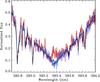 |
Fig. 2 Comparison of the solar spectrum (black) to two seismic solar analogs, KIC 4914923 (blue) and KIC 5774694 (red), around the Ca K line observed with the Hermes spectrograph and illustrative to stars with different magnetic activity levels and ages. |
The values of the index measured for the 18 seismic solar analogs and converted into the MWO system are reported in Table 3. For each star, the index was obtained by taking the mean value of the indices calculated for each unnormalized individual spectrum, while the quoted uncertainties correspond to their associated dispersion. Except for KIC 3241581 (ΔT = 504 days) and KIC 10644253 (ΔT = 180 days), the Hermes observations analyzed here cover a period ΔT of about 35 days over two observing runs (see Sect. 3.2). Over such short interval of time, the scatter between spectra will be mainly related to the instrumental systematics and the weather conditions, while the possible signature of temporal magnetic variations would remain smaller. We note also that in the case of two stars, only one spectrum could be used and that in consequence no dispersion on their index is quoted in Table 3. Furthermore, to characterize the quality of the individual observations, the signal-to-noise ratio in the near UV, S/N(Ca), was estimated for each spectrum at the center of the 90th échelle order at about 400 nm. The mean values of S/N(Ca) are also given in Table 3. We found that the 5 stars with an observed S/N(Ca) < 15 show larger dispersions of their measured index, unlike the 13 stars which higher S/N(Ca). This empirical threshold in S/N(Ca) provides the limit for which the observational and stellar noise dominate the outcome of the formalism.
5.2. Comparison with previous measurements
Three stars of our Kepler sample were observed with the Nordic Optical Telescope (NOT) over the period 2010–2012 and their index measured by Karoff et al. (2013). One of these stars was also measured in 2010 as part of the sample by the California Planet Search program (Isaacson & Fischer 2010). The corresponding values are given in Table 5 and compared to the ones measured in this work with the Hermes spectrograph in June–July 2015. However, we need to keep in mind that the comparison of the index derived from different spectrographs is affected by the associated observational, instrumental, and methodological uncertainties as well as by the corresponding derived instrumental scale factor. For KIC 4914923 and KIC 9098294, the two candidates for a binary system detected in this work (see Table 4), the values of the index reported by Karoff et al. (2013) are smaller than the ones measured here, which would indicate an increase of their magnetic activity in the last few years of about 23% and 35% respectively. The case of the system KIC 9098294 is particularly intriguing because a relatively large variation in radial velocity (ΔRV = 41.35 km s-1) was measured here within a short period of time (35 days), which is comparable to the variation found in the set of eccentric binary systems studied with the Hermes spectrograph by Beck et al. (2014). At the current moment and without the knowledge of the orbital period and the eccentricity of this system, it can only be speculated if the observed variation in the index between the measurements from Karoff et al. (2013) and this study is connected and modulated with the binarity. Further monitoring is thus needed. On the other hand, the activity of KIC 6116048 seems to have remained stable, as consistent -index values are obtained for the three measurements taken five years apart.
Comparison of the -index values with the ones measured by Karoff et al. (2013) and Isaacson & Fischer (2010).
6. Discussion
6.1. Comparison between Sph and index
The photospheric Sph activity proxy can be easily and quickly calculated from existing space photometric observations for a large number of stars observed simultaneously. Moreover, the available observations offer a length of time sufficient enough to cover periods longer than five stellar rotation necessary to measure the Sph. The estimation of a reliable value of the chromospheric index is however more complex as it requires an important investment in telescope time to acquire enough ground-based spectroscopic observations for each individual target. Furthermore, this is more complicated for these rather faint photometric targets. Additionally, these two proxies measure activity in different stellar regions. It is thus important to understand the relation between the index and the Sph by comparing the behavior of these two proxies for a common set of stars.
The comparison between the photospheric Sph and chromospheric -index magnetic activity proxies derived from the Kepler and Hermes observations respectively is shown in Fig. 3 for the subset of 13 solar analogs with a S/N(Ca) > 15 in the spectroscopic data (see Sect. 5.1). The same color and symbol codes as in Fig. 1 were used, while the size of the symbols is inversely proportional to the rotation period from García et al. (2014). Faster rotators are then represented with bigger symbols. The mean values at minimum and maximum along the solar cycle of the photospheric (Salabert et al., in prep.) and chromospheric (Egeland et al. 2016; Hall & Lockwood 2004) magnetic activity levels are represented respectively by the vertical and horizontal dashed lines. The resulting activity box corresponds to the range of change in solar activity along the 11-yr magnetic cycle. Although the sample of stars is small, Fig. 3 indicates that, within the errors, the Sph and indices are complementary. We note also that the Sph and index proxies were not estimated from contemporaneous Kepler and Hermes observations, introducing a dispersion related to possible temporal variations in the stellar activity. Furthermore, the Sph proxy corresponds to a mean activity level averaged over a long period of time – 1422 days of the Kepler observations between 2009 and 2013 –, while the -index proxy measures the stellar activity over a shorter temporal snapshot. In addition, we recall that the Sph is dependent on the inclination angle and represents a lower limit of the photospheric activity. However, it confirms that the Sph can accompany the classical index for activity studies.
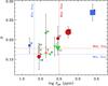 |
Fig. 3 Chromospheric |
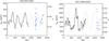 |
Fig. 4 Left panel: photospheric magnetic activity proxy Sph (in ppm, solid black line) of KIC 3241581 estimated from 1422 days of Kepler observations as a function of time. The individual measurements of the |
6.2. Temporal variability in KIC 3241581 and KIC 10644253
In the case of KIC 3241581 and KIC 10644253, for which the time interval, ΔT, of the Hermes observations cover several months, we checked for any possible temporal variations of the index which could be related with variations measured in the Sph. For these two stars, the photospheric Sph shows a clear modulation as a function of time (Fig. 4) and the associated Lomb-Scargle periodograms return a main period of about 394 days for KIC 3241581 and of 582 days for KIC 10644253, the latter being already discussed in Salabert et al. (2016) along comparable variations in the p-mode frequency shifts. The ~1.1-yr variations in KIC 3241581 at a rotation period comparable to the Sun may be analogous to the solar quasi-biennial oscillation observed in various activity proxies (see, e.g., Bazilevskaya et al. 2014, and references therein). Although the associated modulation of about 200 ppm is relatively large, it is however close to the Kepler orbital period. Even though that seems unlikely, we cannot rule out yet any pollution related to the Kepler orbit. The ~1.6-yr variations in the young 1-Gyr-old KIC 10644253 at a rotation period ~11 days previously observed by Salabert et al. (2016) is analogous to what is found by Egeland et al. (2015) in the Mount Wilson star HD 30495, having very close stellar properties and falling on the inactive branch reported by Böhm-Vitense (2007).
The associated individual measurements of the index obtained with the Hermes observations few years after the end of the Kepler mission are represented by the dots in Fig. 4. For both stars, we have also overplotted a sine function calculated using the periodicities given by the Lomb-Scargle analysis above and centered around the first modulation of the Sph. Although this is only qualitative and that it could be related to the intrinsic Hermes instrumental and observational scatter, the -index values for KIC 3241581 show however striking variations which appear to be in close temporal phase with the Sph during two consecutive periods of increasing activity. Only additional spectroscopic observations could confirm these variations in the index, mainly during periods associated to a possible decreasing phase of activity based on Sph. For KIC 10644253, a longer time interval is required because the main periodicity measured in the Sph is larger than the Hermes observations analyzed here.
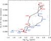 |
Fig. 5 Solar Ca K-line emission as a function of the photospheric magnetic proxy, Sph, ⊙ (in ppm), of the Sun during the solar cycle 23 between 1996 and 2008 (solid line) and smoothed over 1 yr. The first year of cycle 24 is also represented in dashed line. The start of each year is indicated: red for the rising phase and blue for the falling phase of the activity cycle. The individual data points before smoothing are shown in gray. |
6.3. The case of the Sun
To better understand the relation between the photospheric and chromospheric magnetic activity of the solar analogs represented in Fig. 3, we compared the temporal variations of both quantities in the case of the Sun along its 11-yr activity cycle. Unfortunately, no publicly long-term monitoring of the solar index is available. Several scaling relationships were derived to convert the chromospheric Ca K-line emission index of the Sun into index (e.g., Duncan et al. 1991; White et al. 1992; Radick et al. 1998), but they provide different estimates of the solar minima and cycle amplitudes (within 10% and 4% respectively). We thus decided to compare the photospheric Sph, ⊙ proxy of the Sun directly to the Ca K-line emission index measured at Sacramento Peak/National Solar Observatory facility1. Figure 5 shows the solar Ca K-line emission index as a function on a x-log scale of the corresponding Sph, ⊙ calculated from the photometric VIRGO/SPM observations. The period covered corresponds to the entire solar cycle 23 (1996–2008) as in Sect. 4 and Figs. 1 and 3. The nearly daily measurements of Ca K were averaged over the same subseries used to estimate the solar Sph, ⊙ (i.e., 5 × Prot, ⊙ = 125 days with Prot, ⊙ = 25 days). For illustrative purpose in Fig. 5, the data points were smoothed over a period of 1 yr. The individual data points before smoothing are shown in light gray. The start of each year is also indicated. The relationship between the two proxies varies between the rising and falling phases of the solar cycle following an hysteresis pattern. Moreover, a saturation in chromospheric activity is observable during the unusual long and deep activity minimum of cycle 23, which could be associated to the basal chromospheric component as observed in inactive stars and in the quiet Sun (e.g., Schrijver et al. 1989; Schröder et al. 2012; Stenflo 2012). However, this saturation is interestingly not visible in the photospheric activity of the Sun, Sph, ⊙. Nonetheless, such hysteresis has been observed in a wide range of solar observations between photospheric and chromospheric activity proxies, as well as with the p-mode frequency shifts (e.g., Bachmann & White 1994; Jiménez-Reyes et al. 1998; Tripathy et al. 2001; Özgüç et al. 2012). Finally, Fig. 5 supports the complementarity between the photospheric, Sph, and chromospheric, index, proxies observed for the solar analogs in Fig. 3.
6.4. Comparison with Mount Wilson FGK stars
Furthermore, in order to place our sample into context, we assembled a catalog of solar-analog stars with measured Ca ii H and K activity and rotation from the FGK stars observed with the Mount Wilson program (Baliunas et al. 1996; Donahue et al. 1996). In case where measurements were available in both works, values from Donahue et al. (1996) were used. These works give activity averages from synoptic time series lasting up to 30 yr. The values of from our Kepler sample and the MWO stars were converted into the chromospheric emission fraction, , using the prescription of Noyes et al. (1984), based on Tycho-2 (B−V) measurements (see Table 3). The associated uncertainties were derived using standard error propagation methods. The index, , removes the photospheric contribution to the Ca ii H and K bands. The Tycho-2 photometry catalog was obtained from Hipparcos by Høg et al. (2000). A rough selection of solar-analog stars was made by transforming the published (B−V) color index into effective temperature using the scaling relation from Noyes et al. (1984, Eq. (2)): log Teff = 3.908−0.234 × (B−V), and applying the same selection criterium in effective temperature used for the Kepler sample, that is 5520 K ≤ Teff ≤ 6030 K. The final catalog contains 28 MWO solar analogs. Figure 6 shows the activity proxy of the MWO and Kepler solar analogs as a function of their rotation periods. The rotational modulation of the MWO stars was measured directly from their -index time series using a Lomb-Scargle periodogram on bins containing seasonal observations from 150–200 days in length (Donahue et al. 1996). Only the subset of the 13 Kepler solar analogs with a spectroscopic S/N(Ca) > 15 (see Sect. 5.1) is represented.
Our Kepler sample is observed to be in the same vicinity as the MWO sample, which gives additional confidence in our determination of the activity. The MWO stars also show a rough trend of higher activity for faster rotation: unfortunately our Kepler sample lacks of stars rotating faster than 10 days.
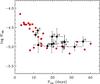 |
Fig. 6 Chromospheric flux ratio, log |


7. Conclusions
The study of the characteristics of the surface activity of solar analogs can provide new constraints in order to better understand the magnetic variability of the Sun, and its underlying dynamo processes, along of its evolution compared to other stars. We thus analyzed here the sample of main-sequence stars observed by the Kepler satellite for which solar-like oscillations were detected (Chaplin et al. 2014) and rotational periods measured (García et al. 2014). Using published stellar parameters derived from the global or the individual asteroseismic properties (Mathur et al. 2012; Chaplin et al. 2014; Metcalfe et al. 2014), we identified 18 seismic solar analogs rotating between 10 and 40 days. We then studied the properties of the photospheric and chromospheric magnetic activity of these stars in relation of the Sun. The photospheric activity proxy, Sph, was derived by means of the analysis of the Kepler observations collected over 1422 days of science operations (from 2009 June 20 to 2013 May 11). The chromospheric activity proxy, index, was measured with follow-up, ground-based spectroscopic observations in 2014 and 2015 with the Hermes instrument mounted to the 1.2 m Mercator telescope in La Palma (Canary Islands, Spain).
Although the size of the sample is rather small, it constitutes the most suitable set of seismic solar analogs which can be identified today with Kepler. In the future, the Transiting Exoplanet Survey Satellite (TESS; Ricker et al. 2015) and PLATO (Rauer et al. 2014) space missions will likely expand this list. Nevertheless, we showed that the magnetic activity of the Sun is comparable to the activity of the seismic solar analogs studied here, within the maximum-to-minimum activity variations of the Sun during the 11-yr cycle. As expected, the youngest and fastest rotating stars are observed to actually be the most active of our Kepler sample, while the activity of stars older than the Sun seems to not evolve much with age.
Furthermore, the comparison of the photospheric Sph with the well-established chromospheric index shows that the Sph index can be used to provide a suitable magnetic activity proxy. Moreover, it can be easily estimated for a large number of stars with known surface rotation observed simultaneously with photometric space missions whose durations cover periods of time longer than five stellar rotation needed to measure the Sph. On the other hand, the estimation of the associated index would be highly difficult to achieve as it would require a lot of time of ground-based telescopes to collect enough spectroscopic data for each individual target. Moreover, these photometric targets are rather faint for spectroscopy observations. Nevertheless, we need to keep in mind that such a photospheric proxy provides a lower limit of the stellar activity because it is dependent on the inclination angle of the rotation axis in respect to the line of sight. This is assuming as well that the starspots are formed over comparable ranges of latitude as in the Sun. Accurate estimates of the inclination angles will be then of great importance in order to provide tighter constraints on the stellar magnetic activity for gyro-magnetochronology studies.
The data from the Ca K-line monitoring program are available at nsosp.nso.edu/node/15
Acknowledgments
The authors wish to thank the entire Kepler team, without whom these results would not be possible. Funding for this Discovery mission is provided by NASA Science Mission Directorate. The ground-based observations are based on spectroscopy made with the Mercator Telescope, operated on the island of La Palma by the Flemish Community, at the Spanish Observatorio del Roque de los Muchachos of the Instituto de Astrofísica de Canarias. This work utilizes data from the National Solar Observatory/Sacramento Peak Ca ii K-line Monitoring Program, managed by the National Solar Observatory, which is operated by the Association of Universities for Research in Astronomy (AURA), Inc. under a cooperative agreement with the National Science Foundation. The research leading to these results has received funding from the European Community’s Seventh Framework Program ([FP7/2007–2013]) under grant agreement No. 312844 (SPACEINN) and under grant agreement No. 269194 (IRSES/ASK). D.S. and R.A.G. acknowledge the financial support from the CNES GOLF and PLATO grants. P.G.B. acknowledges the ANR (Agence Nationale de la Recherche, France) program IDEE (N° ANR-12-BS05-0008) “Interaction Des Étoiles et des Exoplanètes”. R.E. is supported by the Newkirk Fellowship at the High Altitude Observatory. S.M. acknowledges support from the NASA grants NNX12AE17G and NNX15AF13G. T.M. acknowledges support from the NASA grant NNX15AF13G. J.D.N.Jr. acknowledges support from CNPq PQ 308830/2012-1 CNPq PDE Harvard grant. D.S. acknowledges the Observatoire de la Côte d’Azur for support during his stays. This research has made use of the SIMBAD database, operated at CDS, Strasbourg, France.
References
- Appourchaux, T., Chaplin, W. J., García, R. A., et al. 2012, A&A, 543, A54 [NASA ADS] [CrossRef] [EDP Sciences] [Google Scholar]
- Aigrain, S., Llama, J., Ceillier, T., et al. 2015, MNRAS, 450, 3211 [NASA ADS] [CrossRef] [Google Scholar]
- Alvarado-Gómez, J. D., Hussain, G. A. J., Grunhut, J., et al. 2015, A&A, 582, A38 [NASA ADS] [CrossRef] [EDP Sciences] [Google Scholar]
- Bachmann, K. T., & White, O. R. 1994, Sol. Phys., 150, 347 [NASA ADS] [CrossRef] [Google Scholar]
- Baglin, A., Michel, E., Auvergne, M., & The COROT Team 2006, in Proc. SOHO 18/GONG 2006/HELAS I, Beyond the spherical Sun, eds. K. Fletcher, & M. Thompson, ESA SP, 624, 34 [Google Scholar]
- Baliunas, S. L., Hartmann, L., Noyes, R. W., et al. 1983, ApJ, 275, 752 [NASA ADS] [CrossRef] [Google Scholar]
- Baliunas, S. L., Donahue, R. A., Soon, W. H., et al. 1995, ApJ, 438, 269 [NASA ADS] [CrossRef] [Google Scholar]
- Baliunas, S., Sokoloff, D., & Soon, W. 1996, ApJ, 457, L99 [NASA ADS] [CrossRef] [Google Scholar]
- Ballot, J., Appourchaux, T., Toutain, T., & Guittet, M. 2008, A&A, 486, 867 [NASA ADS] [CrossRef] [EDP Sciences] [Google Scholar]
- Basri, G., Walkowicz, L. M., Batalha, N., et al. 2010, ApJ, 713, L155 [NASA ADS] [CrossRef] [Google Scholar]
- Basri, G., Walkowicz, L. M., Batalha, N., et al. 2011, AJ, 141, 20 [NASA ADS] [CrossRef] [Google Scholar]
- Bazilevskaya, G., Broomhall, A.-M., Elsworth, Y., & Nakariakov, V. M. 2014, Space Sci. Rev., 186, 359 [NASA ADS] [CrossRef] [Google Scholar]
- Beck, P. G., Hambleton, K., Vos, J., et al. 2014, A&A, 564, A36 [NASA ADS] [CrossRef] [EDP Sciences] [Google Scholar]
- Beck, P. G., Allen de Prieto, C., Van Reeth, T., et al. 2016, A&A, 589, A27 [NASA ADS] [CrossRef] [EDP Sciences] [Google Scholar]
- Böhm-Vitense, E. 2007, ApJ, 657, 486 [NASA ADS] [CrossRef] [Google Scholar]
- Borucki, W. J., Koch, D., Basri, G., et al. 2010, Science, 327, 977 [NASA ADS] [CrossRef] [PubMed] [Google Scholar]
- Brandenburg, A., Saar, S. H., & Turpin, C. R. 1998, ApJ, 498, L51 [NASA ADS] [CrossRef] [Google Scholar]
- Brun, A. S., García, R. A., Houdek, G., Nandy, D., & Pinsonneault, M. 2015, Space Sci. Rev., 196, 303 [NASA ADS] [CrossRef] [Google Scholar]
- Bruntt, H., Basu, S., Smalley, B., et al. 2012, MNRAS, 423, 122 [NASA ADS] [CrossRef] [Google Scholar]
- Campante, T. L., Chaplin, W. J., Lund, M. N., et al. 2014, ApJ, 783, 123 [NASA ADS] [CrossRef] [Google Scholar]
- Cayrel de Strobel, G. 1996, A&ARv, 7, 243 [CrossRef] [Google Scholar]
- Chaplin, W. J., Bedding, T. R., Bonanno, A., et al. 2011, ApJ, 732, L5 [Google Scholar]
- Chaplin, W. J., Basu, S., Huber, D., et al. 2014, ApJS, 210, 1 [NASA ADS] [CrossRef] [Google Scholar]
- Charbonneau, P. 2010, Liv. Rev. Sol. Phys., 7, 3 [Google Scholar]
- Ceillier, T., van Saders, J., García, R. A., et al. 2016, MNRAS, 456, 119 [NASA ADS] [CrossRef] [Google Scholar]
- Domingo, V., Fleck, B., & Poland, A. I. 1995, Sol. Phys., 162, 1 [NASA ADS] [CrossRef] [Google Scholar]
- Donahue, R. A., Saar, S. H., & Baliunas, S. L. 1996, ApJ, 466, 384 [NASA ADS] [CrossRef] [Google Scholar]
- Doyle, A. P., Davies, G. R., Smalley, B., Chaplin, W. J., & Elsworth, Y. 2014, MNRAS, 444, 3592 [NASA ADS] [CrossRef] [Google Scholar]
- Duncan, D. K., Vaughan, A. H., Wilson, O. C., et al. 1991, ApJS, 76, 383 [NASA ADS] [CrossRef] [Google Scholar]
- Egeland, R., Metcalfe, T. S., Hall, J. C., & Henry, G. W. 2015, ApJ, 812, 12 [NASA ADS] [CrossRef] [Google Scholar]
- Egeland, R., Soon, W., Baliunas, S., et al. 2016, ApJ, submitted [Google Scholar]
- Ferreira Lopes, C. E., Leão, I. C., de Freitas, D. B., et al. 2015, A&A, 583, A134 [NASA ADS] [CrossRef] [EDP Sciences] [Google Scholar]
- Folsom, C. P., Petit, P., Bouvier, J., et al. 2016, MNRAS, 457, 580 [NASA ADS] [CrossRef] [Google Scholar]
- Fröhlich, C., Romero, J., Roth, H., et al. 1995, Sol. Phys., 162, 101 [NASA ADS] [CrossRef] [Google Scholar]
- García, R. A., Mathur, S., Salabert, D., et al. 2010, Science, 329, 1032 [NASA ADS] [CrossRef] [PubMed] [Google Scholar]
- García, R. A., Hekker, S., Stello, D., et al. 2011, MNRAS, 414, L6 [NASA ADS] [CrossRef] [Google Scholar]
- García, R. A., Ceillier, T., Salabert, D., et al. 2014, A&A, 572, A34 [NASA ADS] [CrossRef] [EDP Sciences] [Google Scholar]
- Grec, G., Fossat, E., & Pomerantz, M. 1980, Nature, 288, 541 [NASA ADS] [CrossRef] [Google Scholar]
- Hall, J. C., & Lockwood, G. W. 2004, ApJ, 614, 942 [NASA ADS] [CrossRef] [Google Scholar]
- Hall, J. C., Lockwood, G. W., & Skiff, B. A. 2007, AJ, 133, 862 [NASA ADS] [CrossRef] [Google Scholar]
- Hall, J. C., Henry, G. W., Lockwood, G. W., Skiff, B. A., & Saar, S. H. 2009, AJ, 138, 312 [NASA ADS] [CrossRef] [Google Scholar]
- Hathaway, D. H. 2015, Liv. Rev. Sol. Phys., 12, 4 [Google Scholar]
- Høg, E., Fabricius, C., Makarov, V. V., et al. 2000, A&A, 355, L27 [NASA ADS] [Google Scholar]
- Isaacson, H., & Fischer, D. 2010, ApJ, 725, 875 [NASA ADS] [CrossRef] [Google Scholar]
- Jenkins, J. M., Caldwell, D. A., Chandrasekaran, H., et al. 2010, ApJ, 713, L120 [NASA ADS] [CrossRef] [Google Scholar]
- Jiménez-Reyes, S. J., Régulo, C., Pallé, P. L., & Roca Cortés, T. 1998, A&A, 329, 1119 [NASA ADS] [Google Scholar]
- Karoff, C., Metcalfe, T. S., Chaplin, W. J., et al. 2013, MNRAS, 433, 3227 [NASA ADS] [CrossRef] [Google Scholar]
- Keil, S. L., & Worden, S. P. 1984, ApJ, 276, 766 [NASA ADS] [CrossRef] [Google Scholar]
- Kjeldsen, H., & Bedding, T. R. 1995, A&A, 293, 87 [NASA ADS] [Google Scholar]
- Lockwood, G. W., Skiff, B. A., Henry, G. W., et al. 2007, ApJS, 171, 260 [NASA ADS] [CrossRef] [Google Scholar]
- McQuillan, A., Aigrain, S., & Mazeh, T. 2013, MNRAS, 432, 1203 [NASA ADS] [CrossRef] [MathSciNet] [Google Scholar]
- McQuillan, A., Mazeh, T., & Aigrain, S. 2014, ApJS, 211, 24 [NASA ADS] [CrossRef] [MathSciNet] [Google Scholar]
- Mathur, S., García, R. A., Régulo, C., et al. 2010, A&A, 511, A46 [NASA ADS] [CrossRef] [EDP Sciences] [Google Scholar]
- Mathur, S., Metcalfe, T. S., Woitaszek, M., et al. 2012, ApJ, 749, 152 [NASA ADS] [CrossRef] [Google Scholar]
- Mathur, S., Salabert, D., García, R. A., & Ceillier, T. 2014a, J. Space Weather Space Clim., 4, A15 [NASA ADS] [CrossRef] [EDP Sciences] [MathSciNet] [Google Scholar]
- Mathur, S., García, R. A., Ballot, J., et al. 2014b, A&A, 562, A124 [NASA ADS] [CrossRef] [EDP Sciences] [Google Scholar]
- Metcalfe, T. S., Creevey, O. L., & Christensen-Dalsgaard, J. 2009, ApJ, 699, 373 [NASA ADS] [CrossRef] [Google Scholar]
- Metcalfe, T. S., Creevey, O. L., Doğan, G., et al. 2014, ApJS, 214, 27 [NASA ADS] [CrossRef] [Google Scholar]
- Molenda-Żakowicz, J., Sousa, S. G., Frasca, A., et al. 2013, MNRAS, 434, 1422 [NASA ADS] [CrossRef] [Google Scholar]
- Nielsen, M. B., Gizon, L., Schunker, H., & Karoff, C. 2013, A&A, 557, L10 [NASA ADS] [CrossRef] [EDP Sciences] [Google Scholar]
- Noyes, R. W., Hartmann, L. W., Baliunas, S. L., Duncan, D. K., & Vaughan, A. H. 1984, ApJ, 279, 763 [NASA ADS] [CrossRef] [Google Scholar]
- Pace, G. 2013, A&A, 551, L8 [NASA ADS] [CrossRef] [EDP Sciences] [Google Scholar]
- Petrovay, K. 2010, Liv. Rev. Sol. Phys., 7, 6 [Google Scholar]
- Perryman, M. A. C., de Boer, K. S., Gilmore, G., et al. 2001, A&A, 369, 339 [NASA ADS] [CrossRef] [EDP Sciences] [Google Scholar]
- Pinsonneault, M. H., An, D., Molenda-Żakowicz, J., et al. 2012, ApJS, 199, 30 [NASA ADS] [CrossRef] [Google Scholar]
- Özgüç, A., Kilcik, A., & Rozelot, J. P. 2012, Sol. Phys., 281, 839 [NASA ADS] [CrossRef] [Google Scholar]
- Radick, R. R., Lockwood, G. W., Skiff, B. A., & Baliunas, S. L. 1998, ApJS, 118, 239 [NASA ADS] [CrossRef] [Google Scholar]
- Raskin, G. 2011, Ph.D. Thesis, Institute of Astronomy, Katholieke Universiteit Leuven, Belgium [Google Scholar]
- Raskin, G., van Winckel, H., Hensberge, H., et al. 2011, A&A, 526, A69 [NASA ADS] [CrossRef] [EDP Sciences] [Google Scholar]
- Rauer, H., Catala, C., Aerts, C., et al. 2014, Exp. Astron., 38, 249 [NASA ADS] [CrossRef] [Google Scholar]
- Reinhold, T., & Reiners, A. 2013, A&A, 557, A11 [NASA ADS] [CrossRef] [EDP Sciences] [Google Scholar]
- Ricker, G. R., Winn, J. N., Vanderspek, R., et al. 2015, J. Astron. Telesc. Instrum. Syst., 1, 014003 [NASA ADS] [CrossRef] [Google Scholar]
- Saar, S. H., & Baliunas, S. L. 1992, The Solar Cycle, 27, 150 [Google Scholar]
- Saar, S. H., & Brandenburg, A. 1999, ApJ, 524, 295 [NASA ADS] [CrossRef] [Google Scholar]
- Salabert, D., Jiménez-Reyes, S. J., & Tomczyk, S. 2003, A&A, 408, 729 [NASA ADS] [CrossRef] [EDP Sciences] [Google Scholar]
- Salabert, D., Régulo, C., García, R. A., et al. 2016, A&A, 589, A118 [NASA ADS] [CrossRef] [EDP Sciences] [Google Scholar]
- Schrijver, C. J., Dobson, A. K., & Radick, R. R. 1989, ApJ, 341, 1035 [NASA ADS] [CrossRef] [Google Scholar]
- Schröder, K.-P., Mittag, M., Pérez Martínez, M. I., Cuntz, M., & Schmitt, J. H. M. M. 2012, A&A, 540, A130 [NASA ADS] [CrossRef] [EDP Sciences] [Google Scholar]
- Silva Aguirre, V., Davies, G. R., Basu, S., et al. 2015, MNRAS, 452, 2127 [NASA ADS] [CrossRef] [Google Scholar]
- Soderblom, D. R., Duncan, D. K., & Johnson, D. R. H. 1991, ApJ, 375, 722 [NASA ADS] [CrossRef] [Google Scholar]
- Soon, W. H., Baliunas, S. L., & Zhang, Q. 1993, ApJ, 414, L33 [NASA ADS] [CrossRef] [Google Scholar]
- Skumanich, A. 1972, ApJ, 171, 565 [NASA ADS] [CrossRef] [Google Scholar]
- Stenflo, J. O. 2012, A&A, 547, A93 [NASA ADS] [CrossRef] [EDP Sciences] [Google Scholar]
- Tripathy, S. C., Kumar, B., Jain, K., & Bhatnagar, A. 2001, Sol. Phys., 200, 3 [NASA ADS] [CrossRef] [Google Scholar]
- Vaughan, A. H., Preston, G. W., Baliunas, S. L., et al. 1981, ApJ, 250, 276 [NASA ADS] [CrossRef] [Google Scholar]
- White, O. R., Skumanich, A., Lean, J., Livingston, W. C., & Keil, S. L. 1992, PASP, 104, 1139 [NASA ADS] [CrossRef] [Google Scholar]
- Wilson, O. C. 1978, ApJ, 226, 379 [NASA ADS] [CrossRef] [Google Scholar]
Appendix A: Filter impact on the estimated Sph
The data processing of the photometric Kepler observations can have important impacts on the estimated values of Sph. Indeed, the choice of the high-pass filter applied to the original Kepler data throughout the calibration procedure affects the returned estimates of Sph. For a given star, the Sph will get smaller because the filter bandpass gets narrower as represented on the left panel of Fig. A.1. It shows the median values of Sph calculated for the 310 solar-like stars for which rotation periods, Prot, were measured by García et al. (2014) for different lengths of filter, Nday, applied during the data processing, going from 5 days to 80 days, with 5-day increments. Such dependence for the solar-like oscillating stars was evaluated to be well described by the following
formulation: 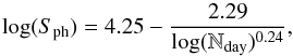 (A.1)where Nday represents the number of days of the applied filter.
The right panel of Fig. A.1 shows the median values of the associated errors of the estimated Sph of the 310 solar-like stars as a function of the filter. For comparison, the red dashed-line shows the difference in Sph between consecutive values of the filter as an indicator of the error introduced by a change in the filter bandpass. For filters 40-day wide upwards, the impact of a change in filter appears to be within the errors on Sph. We decided then to use a filter of Nday = 55 days as the rotation periods of our sample of stars are faster than 40 days.
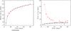 |
Fig. A.1 Left panel: median values of the photospheric activity proxy, Sph (in ppm), calculated for the 310 Kepler solar-like stars for which rotation periods were measured (García et al. 2014) as a function of the length in days of the applied filter F (red dots). The solid line corresponds to the associated fit from Eq. (A.1). Right panel: median values of the associated errors (in ppm) of the estimated Sph of the 310 Kepler solar-like stars as a function of the filter Nday (solid line). The red dashed-line corresponds to the difference in Sph between consecutive values of the filter Nday. |
All Tables
References of the initial Kepler sample of seismic solar-like stars with measured stellar rotation and the identified seismic solar analogs.
Photospheric and chromospheric activity properties of the 18 seismic solar analogs derived from the photometric Kepler and spectroscopic Hermes observations.
Binary systems discovered with the Hermes spectroscopic observations within the sample of seismic solar analogs.
Comparison of the -index values with the ones measured by Karoff et al. (2013) and Isaacson & Fischer (2010).
All Figures
|
Fig. 1 Left panel: photospheric magnetic activity index, Sph (in ppm), as a function of the rotational period, Prot (in days), of the 18 seismic solar analogs observed with the Kepler satellite. The mean activity level of the Sun calculated from the VIRGO/SPM observations is represented for a rotation of 25 days with its astronomical symbol, and its mean activity levels at minimum and maximum of the 11-yr cycle are represented by the horizontal dashed lines. Right panel: same as the left panel but as a function of the seismic age (in Gyr). The position of the Sun is also indicated for an age of 4.567 Gyr. The size of the symbols is inversely proportional to the rotation period, Prot. In both panels, each star is referred by the same number as given in Tables 2 and 3. |
| In the text | |
|
Fig. 2 Comparison of the solar spectrum (black) to two seismic solar analogs, KIC 4914923 (blue) and KIC 5774694 (red), around the Ca K line observed with the Hermes spectrograph and illustrative to stars with different magnetic activity levels and ages. |
| In the text | |
|
Fig. 3 Chromospheric |
| In the text | |
|
Fig. 4 Left panel: photospheric magnetic activity proxy Sph (in ppm, solid black line) of KIC 3241581 estimated from 1422 days of Kepler observations as a function of time. The individual measurements of the |
| In the text | |
|
Fig. 5 Solar Ca K-line emission as a function of the photospheric magnetic proxy, Sph, ⊙ (in ppm), of the Sun during the solar cycle 23 between 1996 and 2008 (solid line) and smoothed over 1 yr. The first year of cycle 24 is also represented in dashed line. The start of each year is indicated: red for the rising phase and blue for the falling phase of the activity cycle. The individual data points before smoothing are shown in gray. |
| In the text | |
|
Fig. 6 Chromospheric flux ratio, log |
| In the text | |
|
Fig. A.1 Left panel: median values of the photospheric activity proxy, Sph (in ppm), calculated for the 310 Kepler solar-like stars for which rotation periods were measured (García et al. 2014) as a function of the length in days of the applied filter F (red dots). The solid line corresponds to the associated fit from Eq. (A.1). Right panel: median values of the associated errors (in ppm) of the estimated Sph of the 310 Kepler solar-like stars as a function of the filter Nday (solid line). The red dashed-line corresponds to the difference in Sph between consecutive values of the filter Nday. |
| In the text | |
Current usage metrics show cumulative count of Article Views (full-text article views including HTML views, PDF and ePub downloads, according to the available data) and Abstracts Views on Vision4Press platform.
Data correspond to usage on the plateform after 2015. The current usage metrics is available 48-96 hours after online publication and is updated daily on week days.
Initial download of the metrics may take a while.