| Issue |
A&A
Volume 595, November 2016
|
|
|---|---|---|
| Article Number | A41 | |
| Number of page(s) | 16 | |
| Section | Numerical methods and codes | |
| DOI | https://doi.org/10.1051/0004-6361/201628205 | |
| Published online | 26 October 2016 | |
APSARA: A multi-dimensional unsplit fourth-order explicit Eulerian hydrodynamics code for arbitrary curvilinear grids
1 RIKEN, Astrophysical Big Bang Laboratory, 2-1 Hirosawa, Wako, 351-0198 Saitama, Japan
e-mail: annop.wongwathanarat@riken.jp
2 Max-Planck-Institut für Astrophysik, Karl-Schwarzschild-Straße 1, 85748 Garching, Germany
3 Institute of Mathematics, University of Vienna, Oskar-Morgenstern-Platz 1, 1090 Vienna, Austria
Received: 28 January 2016
Accepted: 11 July 2016
We present a new fourth-order, finite-volume hydrodynamics code named Apsara. The code employs a high-order, finite-volume method for mapped coordinates with extensions for nonlinear hyperbolic conservation laws. Apsara can handle arbitrary structured curvilinear meshes in three spatial dimensions. The code has successfully passed several hydrodynamic test problems, including the advection of a Gaussian density profile and a nonlinear vortex and the propagation of linear acoustic waves. For these test problems, Apsara produces fourth-order accurate results in case of smooth grid mappings. The order of accuracy is reduced to first-order when using the nonsmooth circular grid mapping. When applying the high-order method to simulations of low-Mach number flows, for example, the Gresho vortex and the Taylor-Green vortex, we discover that Apsara delivers superior results to codes based on the dimensionally split, piecewise parabolic method (PPM) widely used in astrophysics. Hence, Apsara is a suitable tool for simulating highly subsonic flows in astrophysics. In the first astrophysical application, we perform implicit large eddy simulations (ILES) of anisotropic turbulence in the context of core collapse supernova (CCSN) and obtain results similar to those previously reported.
Key words: methods: numerical / hydrodynamics / turbulence
© ESO, 2016
1. Introduction
In many astrophysical simulations, such as simulations of convection inside a star and stellar explosions, spherical coordinates are often a preferable choice for integrating the respective partial differential equations. However, the spherical polar coordinates possess coordinate singularities at the coordinate origin and along the north and south poles, which prevent an easy and straightforward implementation of numerical methods. These coordinate singularities result in smaller time steps and, hence, special numerical treatments and/or boundary conditions have to be applied. This leads to a degradation of the efficiency of the employed numerical schemes and may introduce numerical artifacts.
For example, in recent state-of-the-art, three-dimensional (3D) simulations of core collapse supernovae (CCSN) performed with time-explicit, finite-volume hydrodynamic codes (e.g., Melson et al. 2015a; Lentz et al. 2015), the flow is modeled in spherical symmetry inside a specified sphere representing the inner core of the proto-neutron star, where the symmetry assumption is justified, to alleviate the restriction of the time step due to the Courant-Friedrichs-Lewy (CFL) condition. In addition, a reflecting boundary condition is usually applied at the coordinate origin. Müller (2015) applied the same spherical symmetry assumption, but he also included the effect of proto-neutron star convection by means of a mixing-length theory (e.g., Wilson & Mayle 1988). Lentz et al. (2015) avoided time steps that were too small by using nonuniform angular zones in the polar direction and an azimuthal averaging procedure for grid zones near the two poles. Similarly, Müller (2015) circumvented this problem using a mesh coarsening scheme in 30° cones around the poles whereby the short wavelength noise in the azimuthal direction is filtered out.
The problem of the severe time step restriction near the singular points at the poles of a sphere, also known as the pole-problem, has received much attention in various fields of research over the past few decades. In the particular case of finite-volume methods on a structured mesh, two popular solutions to the pole-problem are the cubed sphere grid (Ronchi et al. 1996) and the Yin-Yang grid (Kageyama & Sato 2004). The cubed sphere grid is based on a projection of the six sides of a cube onto the surface of a sphere and thus consists of six equidistant (in polar and azimuthal direction) identical grid patches. Except for the one point at the middle of each grid patch, the cubed sphere mesh is nonorthogonal. On the other hand, the Yin-Yang grid is formed by combining two identical low-latitude parts of a spherical polar grid. Hence, it is orthogonal everywhere, allowing for an easy extension of existing numerical codes that are based on an orthogonal mesh. Nevertheless, overlapping grids like the Yin-Yang grid have a drawback. Even if the numerical scheme employed on each grid patch is conservative, this does not ensure global conservation in the computational volume unless one applies a flux correction algorithm at the boundaries between the two grid patches (see, e.g., Peng et al. 2006; Wongwathanarat et al. 2010). In contrast, the boundaries of each patch of the cubed sphere mesh coincide perfectly with its neigboring patches, i.e., there is no overlap between grid patches. Thus, boundary flux corrections can be implemented in a more straightforward manner than in the case of the Yin-Yang grid.
Both the cubed sphere grid and the Yin-Yang grid have been used in various astrophysical applications. For instance, the cubed sphere grid was applied in simulations of accretion flows onto magnetized stars (e.g., Koldoba et al. 2002; Romanova et al. 2012) and accretion disks around rotating black holes (Fragile et al. 2009). The Yin-Yang grid was used, for example, in CCSN simulations (e.g., Wongwathanarat et al. 2015; Melson et al. 2015b), simulations of type Ia supernova remnants (Warren & Blondin 2013), and calculations of the solar global convection (Hotta et al. 2014), solar corona (e.g., Jiang et al. 2012; Feng et al. 2012), and coronal mass ejections (Shiota et al. 2010).
While the cubed sphere grid and the Yin-Yang grid circumvent the pole-problem, the singularity at the coordinate origin remains in both cases. One possible solution is to supplement the cubed sphere mesh or the Yin-Yang mesh with a Cartesian mesh at small radii to cover the central part of the sphere. An example of such a grid arrangement, called the Yin-Yang-Zhong, was recently developed by Hayashi & Kageyama (2016). Using this approach, the numerical code must be able to deal with different coordinate systems on different grid patches. In addition, global conservation is hampered by the overlap of the Cartesian grid patch with the spherical grid patches. On the other hand, the GenASiS code developed by Cardall et al. (2014) handles both the pole-problem and the singularity at the coordinate origin by employing the adaptive mesh refinement (AMR) approach. Instead of a block-structured AMR framework, GenASiS uses a more flexible cell-by-cell refinement in the Cartesian coordinate system. The cell-by-cell refinement can generate a centrally refined mesh, achieving higher and higher resolutions toward the origin of the sphere, which is a desirable grid property for many astrophysical applications. Nevertheless, a possible disadvantage of the cell-by-cell refinement approach is the cost of a complicated data communication on large-scale machines.
Calhoun et al. (2008) proposed grid mappings for circular or spherical domains that work on a logically rectangular mesh. These grid mappings can be used together with the mapped-grid technique in which one formulates the governing equations in an abstract (singularity-free) computational space instead of in a physical space and applies a coordinate transformation between them. A great advantage of the mapped-grid approach is that the computational domain can always be discretized by an equidistant Cartesian mesh. Therefore, any numerical scheme formulated for a Cartesian equidistant grid can be applied in a straightforward manner. The mapped-grid technique is widely used in engineering applications, where complicated geometries are common (see, e.g., LeVeque 2002). In the field of astrophysics, the mapped-grid approach is not very well known and has only been used up to now in a few numerical codes (Kifonidis & Müller 2012; Grimm-Strele et al. 2014; Miczek et al. 2015).
Colella et al. (2011) introduced a new class of high-order (better than second-order), finite-volume methods for mapped coordinates. The methods are based on computing face-averaged fluxes at each face of a control volume using high-order quadrature rules rather than the mid-point rule as in standard second-order accurate schemes. They demonstrated the capability of their approach to solve an elliptic equation and a scalar, linear hyperbolic equation up to fourth-order accuracy. An extension of the method to solve nonlinear hyperbolic equations was presented for Cartesian coordinates by McCorquodale & Colella (2011) and for mapped coordinates by Guzik et al. (2012). This extension is nontrivial because it is necessary to perform nonlinear transformations between point and (zone and face) averaged values of the conserved variables and fluxes ensuring fourth-order accuracy.
Motivated by the works of Calhoun et al. (2008) and Colella et al. (2011), we have developed a new numerical code for astrophysical applications. This code, which we named Apsara, is based on the fourth-order implementation of the high-order, finite-volume method in mapped coordinates by Colella et al. (2011). The code is extended to solve the Euler equations of gas dynamics using a high-resolution, shock-capturing (HRSC) method on arbitrary, structured curvilinear grids in three spatial dimensions as described in Guzik et al. (2012). This code robustly captures shock waves and discontinuities, while obtaining high-order accurate results in smooth flow regions. On the other hand, simulations of flows on complex grid geometry are possible thanks to the mapped-grid technique. These combined features make the code suitable for simulating a wide range of astrophysical problems.
The paper is organized as follows. In Sect. 2, we summarize the methods by Colella et al. (2011), McCorquodale & Colella (2011), and Guzik et al. (2012) for simulating 3D compressible flows in mapped coordinates. In Sect. 3, examples of mapping functions are introduced, which are employed in our test calculations. In Sect. 4, using a set of hydrodynamic tests, we demonstrate the capability of Apsara to compute fourth-order accurate solutions for smooth flows without discontinuities. In addition, we show the ability of Apsara to accurately calculate low-Mach number flows. As an astrophysical application, we also performed turbulence simulations in the context of CCSN with Apsara. We discuss the results of these simulations in Sect. 5. Finally, we summarize the code properties in Sect. 6, and mention some plans for future extensions of Apsara.
2. Numerical methods
2.1. Governing equations
The Euler equations written in Cartesian coordinates (x,y,z) in three spatial dimensions read 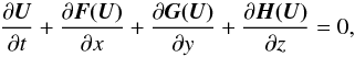 (1)where the vector of conserved variables U and the Cartesian flux functions F, G, and H are given by
 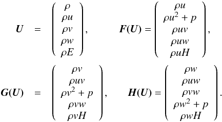 (2)The hydrodynamic state variables in Eq. (2) are the density ρ, the Cartesian components of the velocity field v = (u,v,w)T, the pressure p, the specific total enthalpy
  (3)and the specific internal energy e. The pressure p is related to ρ and e via the equation of state (EOS) of a perfect gas
  (4)where γ is the adiabatic index.
We solve Eq. (1) using a finite-volume approach. The domain of interest is discretized into small subvolumes Vi, where the subscript i = (i,j,k) are indices referring to the ith, jth, and kth cell in each coordinate direction. We integrate Eq. (1) for each of the control volumes Vi to obtain the Euler equations in their integral form. For each component of the vector of conserved variables U we have  (5)where Us denotes the sth component of U, and Fs = (Fs,Gs,Hs)T is the corresponding flux vector. We then define a mapping function M, which maps coordinates ξ = (ξ,η,ζ)T one-to-one in an abstract computational space into coordinates x = (x,y,z)T in physical space, i.e.,
  (6)For simplicity we discretize the computational space with a Cartesian mesh consisting of computational cells Ωi, which are unit cubes. The mapping function M is defined such that the image M(Ωi) of each computational cell Ωi corresponds to the control volume Vi in physical space. By applying the change of variables theorem (see, e.g., Appel 2007) to Eq. (5), the integrals over a control volume Vi in physical space are transformed into integrals over a computational cell Ωi according to
  (7)where
  (8)is the Jacobian determinant of the inverse mapping M-1. The divergence of Fs can be expressed in terms of derivatives in the computational space (Colella et al. 2011),
 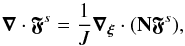 (9)the matrix N being defined as
 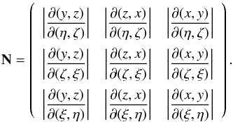 (10)Using Eq. (9) we obtain from Eq. (7)
 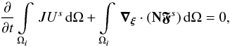 (11)which resembles Eq. (5). Applying the divergence theorem Eq. (11) becomes
 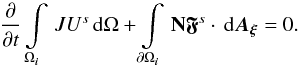 (12)The second integral in Eq. (12) is performed over all faces ∂Ωi of a cell Ωi, where Aξ is the surface vector of each cell face pointing in the outward normal direction. The integrals in Eq. (12) are approximated to fourth-order accuracy as
 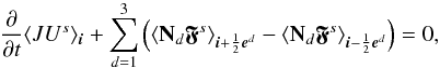 (13)where ed is the unit vector in the dth direction and Nd is the dth row of the matrix N. The operators ⟨ ·⟩ i and
  denote the fourth-order accurate approximations of volume averages and face averages, respectively. We omit factors of h3 and h2 multiplying the first and second term, respectively, on the LHS of Eq. (13) owing to the cell spacing h = 1.
2.2. Temporal discretization
In accordance with our fourth-order accurate spatial scheme, we use a fourth-order accurate Runge-Kutta (RK4) scheme for the time integration. Discretizing the time derivative in Eq. (13) one obtains the following update formula for the cell averaged conserved quantities ⟨ JUs ⟩ i, 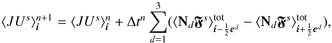 (14)where
  and
and  represent the cell averaged conserved quantities at times tn and tn + 1 = tn + Δtn, respectively. The total RK4 face averaged fluxes
  are given by the linear combination
 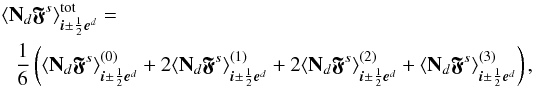 (15)where
 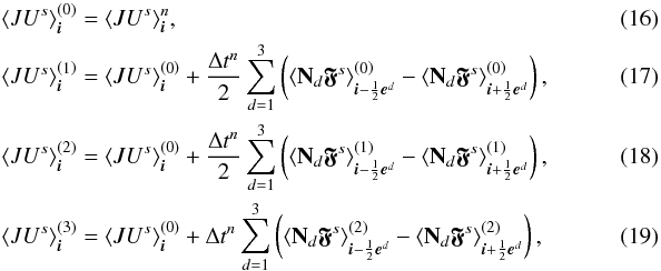 and
and  (20)The size of the time step Δt is given by the condition (McCorquodale & Colella 2011)
  (21)where cs is the speed of sound.
2.3. Cell and face averages
A fourth-order approximation of the cell average of a function f on a mapped grid can be computed by performing a Taylor expansion of the function about the cell center in the computational space. The expansion yields  (22)where fi denotes the pointwise value of f at the center of Ωi. Because the Laplacian operator in Eq. (22) only needs to be evaluated to second-order accuracy, we use the second-order accurate central difference formula to calculate it. On the equidistant Cartesian grid in the computational space, we define the quantities
  (23)to calculate the cell averages of a function f as
  (24)Conversely, we can obtain a fourth-order approximation of the fi from cell averages ⟨ f ⟩. In this case, the Laplacian is calculated using cell averages ⟨ f ⟩, which yields
  (25)Similarly, expanding f about the center of a cell face in the dth direction, we obtain fourth-order accurate face values
  (26)where
  denotes the transverse Laplacian operator. As before, we replace the transverse Laplacian by
  (27)to obtain
  (28)To calculate pointwise values of f at face centers from face averages we use
  (29)In addition, we also need expressions for cell averages and face averages of a product of two functions, for example, for the products JUs and NdFs that appear in the update formula (Eq. (13). The Taylor expansion of the product of two functions f and g about the cell center gives
  (30)where the first-order partial derivatives can be replaced again by second-order accurate central differences. We define
  (31)and compute ⟨ fg ⟩ i as
  (32)Similarly, the face averages are given by
 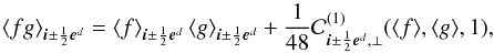 (33)where
 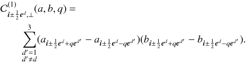 (34)Using Eq. (33) we can write the face average fluxes as
 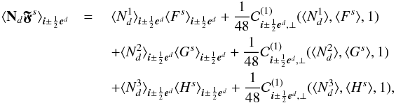 (35)where
  , with c = 1,2,3, is the cth component of the row matrix Nd.
The way one calculates  is an important step for a hydrodynamics code using a curvilinear grid, since it determines the freestream preservation property of the code. Consider a uniform initial state with ρ = p = 1 and u = v = w = 0 at every grid point. All conserved quantities do not change with time for such a state. Therefore, it follows from Eqs. (14) and (35) that
 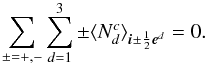 (36)This condition is equivalent to the geometric identity that the sum of the surface normal vectors over all faces of a closed control volume must be zero. Violation of the freestream condition leads to errors that can destroy the numerical solution completely (see, e.g., Grimm-Strele et al. 2014).
If we define a matrix  by (Colella et al. 2011)
 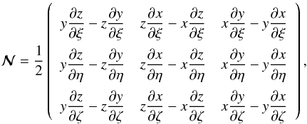 (37)it follows that
 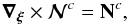 (38)where
  and Nc are the cth column of the matrices and N, respectively. Using Eq. (38) and Stoke’s theorem, the face average becomes
 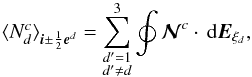 (39)where Eξd is the right-handed tangent vector of the (hyper) edges of the cell face in the dth direction. For instance,
 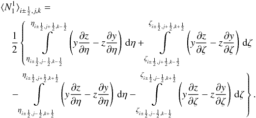 (40)To calculate , we apply Simpson’s rule to calculate the integrals in Eq. (39) and we approximate the first-order derivatives by second-order accurate finite differences. For example, the first integral on the right-hand side (RHS) of Eq. (40) is then given by
 ![\begin{eqnarray} &&\int\limits_ {\eta_{i\pm\frac{1}{2},j-\frac{1}{2},k-\frac{1}{2}}}^ {\eta_{i\pm\frac{1}{2},j+\frac{1}{2},k-\frac{1}{2}}}\, \left( y\frac{\partial z}{\partial\eta} - z\frac{\partial y}{\partial\eta} \right)\,\mrm{d}\eta = \nonumber\\ &&\quad\frac{1}{6}[y_{i\pm\frac{1}{2},j+\frac{1}{2},k-\frac{1}{2}} ( 3z_{i\pm\frac{1}{2},j+\frac{1}{2},k-\frac{1}{2}} -4z_{i\pm\frac{1}{2},j,k-\frac{1}{2}} + z_{i\pm\frac{1}{2},j-\frac{1}{2},k-\frac{1}{2}}) \nonumber\\ && \quad +4y_{i\pm\frac{1}{2},j,k-\frac{1}{2}} ( z_{i\pm\frac{1}{2},j+\frac{1}{2},k-\frac{1}{2}} - z_{i\pm\frac{1}{2},j-\frac{1}{2},k-\frac{1}{2}}) \nonumber\\ && \quad+ y_{i\pm\frac{1}{2},j-\frac{1}{2},k-\frac{1}{2}} (-3z_{i\pm\frac{1}{2},j+\frac{1}{2},k-\frac{1}{2}} +4z_{i\pm\frac{1}{2},j,k-\frac{1}{2}} - z_{i\pm\frac{1}{2},j-\frac{1}{2},k-\frac{1}{2}}) \nonumber\\ && \quad - z_{i\pm\frac{1}{2},j+\frac{1}{2},k-\frac{1}{2}} ( 3y_{i\pm\frac{1}{2},j+\frac{1}{2},k-\frac{1}{2}} -4y_{i\pm\frac{1}{2},j,k-\frac{1}{2}} + y_{i\pm\frac{1}{2},j-\frac{1}{2},k-\frac{1}{2}}) \nonumber\\ && \quad -4z_{i\pm\frac{1}{2},j,k-\frac{1}{2}} ( y_{i\pm\frac{1}{2},j+\frac{1}{2},k-\frac{1}{2}} - y_{i\pm\frac{1}{2},j-\frac{1}{2},k-\frac{1}{2}}) \nonumber\\ && \quad - z_{i\pm\frac{1}{2},j-\frac{1}{2},k-\frac{1}{2}} (-3y_{i\pm\frac{1}{2},j+\frac{1}{2},k-\frac{1}{2}} +4y_{i\pm\frac{1}{2},j,k-\frac{1}{2}} - y_{i\pm\frac{1}{2},j-\frac{1}{2},k-\frac{1}{2}})]. \end{eqnarray}](/articles/aa/full_html/2016/11/aa28205-16/aa28205-16-eq102.png) (41)Using the relation ∇·x = 3, we compute ⟨ J ⟩ i with the help of Eq. (9). Integrating over the cell volume, we obtain
(41)Using the relation ∇·x = 3, we compute ⟨ J ⟩ i with the help of Eq. (9). Integrating over the cell volume, we obtain 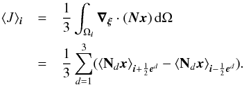 (42)The face averages
  can be computed in a similar manner as the face average fluxes
  in Eq. (35). With the help of Eq. (30) we write
 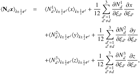 (43)where the face averages
  ,
,  and
and  are given by the expressions
 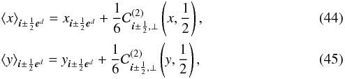 and
and 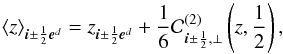 (46)respectively. The first-order derivatives of , x, y, and z appearing in the sums in Eq. (43) are computed as follows. To calculate
  , for instance, we have
  (47)Approximating the first and second derivatives in this expression by second-order accurate finite differences, we obtain
 (48)The derivatives of x, y, and z are approximated by central differences, i.e.
 , for instance, is given by
  (49)When using Eqs. (44)–(49) to calculate the face averages, do not require any data from neighboring cells.
2.4. Evaluation of face average fluxes
To obtain the face average fluxes  ,
,  , and
, and  , we follow the procedure described in detail by (McCorquodale & Colella 2011), which we summarize in the following:
-
1.
Compute ⟨ Us ⟩ i from ⟨ JUs ⟩ i using Eq. (32)
 (50)However, because ⟨ Us ⟩ is not yet known, use instead
  (51)
(51) -
2.
Obtain the pointwise value
 at the cell center using Eq. (25).
 -
3.
Convert Ui to Wi using the EOS, where W = (ρ,u,v,w,p)T is the vector of primitive variables.
-
4.
Calculate the cell average ⟨ Ws ⟩ i from Wi using Eq. (24).
-
5.
Reconstruct the face average
 from the cell average ⟨ Ws ⟩ i using the expression
  (52)
(52) -
6.
Apply a limiter to the interpolated value
as described in Sect. 2.4.1 in McCorquodale & Colella (2011). This limiter is a variant of the smooth extrema preserving limiter by Colella & Sekora (2008), which was proposed as an improvement to the limiter for the piecewise parabolic method (PPM) in Colella & Woodward (1984). The application of the limiter leads to two different values at cell faces,  and
and  , in regions where the interpolated profiles are not smooth.
 -
7.
Solve a Riemann problem at each cell face with
 and
and  as the left and right state, respectively. In Apsara we utilize the exact Riemann solver for real gases of Colella & Glaz (1985).
 -
8.
Compute
 at the face centers from the solution of the Riemann problem using Eq. (29).
 -
9.
Use
to compute  .
. -
10.
Calculate
, , and from using Eq. (28).
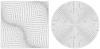 |
Fig. 1 Examples of 2D meshes generated using smooth mapping M1 (left) and circular mapping M2 (right). |
3. Mapping functions
Apsara is capable of integrating the Euler equations on arbitrary curvilinear structured grids using the mapped grid technique. To perform the test problems that we present in Sect. 4 we used three different grid mappings. The computational space is discretized with an equidistant Cartesian mesh for each grid mapping, in which the grid spacing is unity in the three coordinate directions ξ, η, and ζ. The edge lengths of the computational domain are therefore  (53)where Nξ,Nη, and Nζ are the number of grid cells in the ξ, η, and ζ direction. We define normalized coordinates in computational space by
 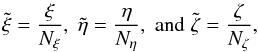 (54)and we choose the coordinates of the inner (i.e., left) grid boundaries in computational space to be ξib = ηib = ζib = 0.
3.1. Cartesian mapping M0
In this simplest case, the coordinates (ξ,η,ζ) in computational space are mapped to physical space by  where xib/ob,yib/ob, and zib/ob denote the coordinates of the inner/outer grid boundaries in physical space in the x,y, and z direction, respectively.
3.2. Smooth mapping M1
For the test problems performed in a rectangular domain, we used a nonlinear mapping given in Colella et al. (2011). The mapping function is defined as 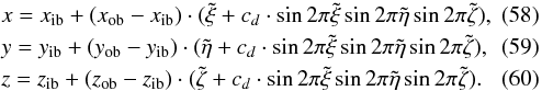 This mapping function results in a smoothly deformed Cartesian mesh shown in the left panel of Fig. 1. The deformation is controlled by the parameter cd. In all test problems, where we applied this smooth mapping, we set cd equal to 0.1.
3.3. Circular mapping M2
For the 2D test problems simulated in a circular domain, we used the singularity-free mapping function proposed by Calhoun et al. (2008), which is defined by 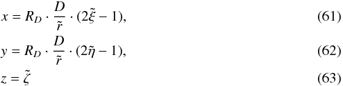 with
with 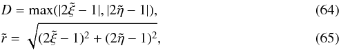 where RD is the radius of the circular domain in physical space. This mapping function maps concentric squares in computational space to circular shells in physical space. As a result grid cells near the diagonals of the squares are severely distorted. An example of such a mesh is depicted in the right panel of Fig. 1.
4. Hydrodynamic tests
L1 and L∞ errors of ⟨ ρ ⟩, and the convergence rates for the 1D linear advection test.
4.1. Linear advection
We performed one-dimensional (1D) and two-dimensional (2D) advection tests, where a Gaussian density profile 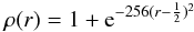 (66)is advected with a constant velocity through a domain of size [0,1] (1D) and [0,1] × [0,1] (2D), respectively. In the 1D test r = x−x0 and v = (1.0,0.0,0.0)T, while r2 = (x−x0)2 + (y−y0)2 and v = (1.0,0.5,0.0)T in the 2D test. We placed the center of the Gaussian profile at (x0,y0) = (0.5,0.5) and imposed periodic boundary conditions in each coordinate direction.
While we employed a single grid with a constant spacing in the 1D test, we used two different meshes in the 2D tests: the Cartesian mesh M0, and the smoothly deformed mesh M1. We followed the advection of the Gaussian profile for two time units in 2D and for ten time units in 1D to compare our 1D results with those of McCorquodale & Colella (2011). The Gaussian profile returned to its original position at the end of each simulation. We set the CFL number to 0.2 and used the ideal gas EOS with  .
.
We computed the L1 and L∞ norms of ⟨ ρ ⟩ from the simulation results, using ⟨ ρ ⟩ at time t = 0 as the reference solution. These norms, together with the corresponding convergence rates, are given in Tables 1 and 2 for the 1D and 2D simulations, respectively. In these tables we also give the results that we computed with the Prometheus code (Fryxell et al. 1991; Mueller et al. 1991).
For the 1D linear advection test as well as for the 2D test with M0 and M1, we find that Apsara shows 4th-order convergence according to both the L1 and the L∞ norm. The convergence rates for grid sizes below 256 zones in 1D and 2562 zones in 2D are less than fourth order because at these grid resolutions the Gaussian profile is not well enough resolved. The L1 and L∞ errors are almost exactly the same in our 1D Apsara simulations as those obtained by McCorquodale & Colella (2011). The L1 and L∞ errors computed with Prometheus show convergence rates below third order. This results partly from the fact that the original PPM limiter implemented in Prometheus fails to preserve the extremum of the Gaussian profile (Colella & Sekora 2008). Because the limiter implemented in Apsara is similar to the extremum-preserving limiter proposed by Colella & Sekora (2008), clipping of extrema is considerably reduced in Apsara. We demonstrate this in Fig. 2, where the density profiles are plotted for 1D simulations that are performed with both codes on a grid of 128 grid cells.
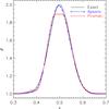 |
Fig. 2 Density profiles for the 1D linear advection test obtained on a grid of 128 zones at t = 10. Results computed with Apsara and Prometheus are shown with blue crosses and red circles, respectively. The exact solution is shown in black. |
4.2. Linear acoustic wave
In this test we simulated the propagation of a sound wave as described in Stone et al. (2008) in 1D, 2D, and 3D using the smooth mapping M1 and the ideal gas EOS with . The background fluid has a density ρ0 = 1, a pressure  , and is initially at rest. We introduced a perturbation vector
  (67)which here only depends on the coordinate x, but in principle could depend on the other coordinates as well. We used an amplitude A = 10-6 to perturb the conserved variables U0 of the background fluid. The domain size was set equal to one wavelength of the pertubation, i.e., the size of the domain in each coordinate direction was unity.
Imposing periodic boundary conditions in all directions and using a CFL number of 1.3, we evolved the flow for one time unit so that the wave propagated once across the domain. In multi-D we also performed simulations using a second-order version of Apsara for comparison. This required an easy modification of the code, where one omits the second order correction terms when calculating face average fluxes. We used the RK4 scheme for time integration for both the fourth-order and second-order accurate code version. Reducing the order of the spatial discretization to second order was sufficient to downgrade the overall convergence from fourth order to second order, i.e., the accuracy of the code is dominated by spatial discretization errors in this test.
As described in Stone et al. (2008), we also computed the L1 error for each component of the conserved variables U using the pointwise values at the cell centers. Fourth-order accurate approximations of these pointwise values of Us were calculated as described in steps 1 and 2 in Sect. 2.4. Following these steps is essential when one wants to achieve fourth-order convergence. If one computes the L1 errors without distinguishing between pointwise values and cell average values, one observes only second-order convergence even though the numerical scheme is of higher order. Table 3 gives the sum of the L1 errors of all conserved variables 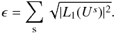 (68)This table also shows that the fourth-order implementation of Apsara achieves the design convergence rate only at low resolution, i.e., up to about 128 grid points per coordinate direction, while at higher resolutions the convergence rate drops dramatically. This is not unexpected because the reference solution used for computing the errors is only a solution of the linearized Euler equations. Hence, the convergence rate starts to degrade when the errors reach a level of A2 ~ 10-12 and nonlinear terms can no longer be neglected. On the other hand, second-order convergence is achieved with the second-order version of Apsara as expected, but here the convergence rate also degrades in 2D at high resolutions when ϵ ~ 10-12.
To demonstrate that fourth-order convergence is indeed achieved with Apsara, we calculated the L1 norm of the coarse-fine differences of the cell center values of ρ for different grid resolutions. More precisely, we first computed a fourth-order approximation of ρ at the cell centers of a coarser grid from the values given on the next finer grid, and then computed the differences between these cell center values and those obtained on the coarser grid. We refer to Appendix A for a more detailed explanation of this coarse-fine interpolation. The results shown in Table 4 indeed confirm the fourth-order convergence of the coarse-fine differences in ρ. In 2D, the convergence rate decreases slightly when comparing results from simulations with 5122 and 10242 grid points owing to numerical round-off errors. As expected the second-order accurate implementation of Apsara yields second-order convergence.
L1-norm of the coarse-fine differences of the pointwise densities ρ as a function of grid resolution for the linear acoustic wave test.
4.3. Advection of a nonlinear vortex
In this 2D test problem we simulated the advection of an isentropic vortex with a uniform backgroud flow, following Yee et al. (2000). The background flow has a density, pressure, and temperature ρ0 = p0 = T0 = 1, and moves with velocities u0 = v0 = 1. The isentropic vortex is added to the freestreaming background flow by introducing perturbations in velocity and temperature, which are given by 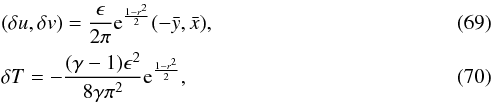 where ϵ is a free parameter regulating the vortex strength, and
  . The coordinates
  are measured from the center of the vortex located at (x0,y0). We chose ϵ = 5, and used the ideal gas EOS with γ = 1.4 for this test. After adding the perturbation
 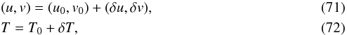 all conserved quantities can be calculated using the fact that the flow is isentropic.
We performed this test on a 2D rectangular domain [−10,10] × [−10,10] using the mapping function M1, and also on a 2D circular domain of radius RD = 10 using the circular mapping function M2. We assume a free outflow boundary in both coordinate directions. The vortex is initially placed at (x0,y0) = (−1,−1). We follow the advection of this vortex for two time units with a CFL number of 1.3. The analytic solution tells one that the center of the vortex is located at (x,y) = (1,1) at the end of the simulations. We computed the L1 and L∞ norms of the errors of the pointwise value of the density ρ at the cell center (see Table 5).
The results from the simulations performed on the M1 grid show fourth-order convergence in both the L1 and L∞ norm. In contrast, the convergence order is reduced significantly on the M2 grid. This illustrates that the accuracy and convergence rate of the fourth-order scheme implemented in Apsara is degraded when using a mapping function that is nonsmooth. Grimm-Strele et al. (2014) also performed the same test problem with the same M2 mapping function, using the weighted essentially nonoscillatory (WENO) finite volume scheme. They also found a reduced convergence rate for the M2 grid in comparison with the smooth mapping M1. We speculate that the convergence rate on the grid M2 is destroyed by the very poor mesh quality along the diagonals since the angle between two adjacent cell sides is nearly 180° for grid cells there.
L1 and L∞ errors of ρ, and their convergence rates for the 2D advection of a nonlinear vortex test.
4.4. Influence of grid smoothness
In many astrophysical simulations in spherical geometry one usually employs logarithmic spacing for grid cells in the radial direction to cover large spatial length scales. For example, the grid spacing of a radial zone i, Δri, can be written as  (73)where Δri−1 is the grid size of zone i−1, Nr is the number of radial grid zones, and α is the grid expansion ratio. If α is too large, the grid can be considered as nonsmooth and, as a result, the order of accuracy of the employed numerical scheme is degraded. Therefore, in this section we systematically study the influence of the smoothness of the mapping function on the performance of Apsara to determine approximately the maximum grid expansion ratio allowed in the case of a nonequidistant grid spacing without losing fourth-order convergence.
To this end, we considered the isentropic vortex test described in Sect. 4.3 on a 2D mesh with variable grid spacing in one coordinate direction. The 2D mesh used for this test is designed in the following way. Firstly, we defined two grid spacing parameters: δ1 = 2Lx/Nξ and δ2 = 2Lx/ 3Nξ, where Lx is the domain size in the x direction. The parameters δ1 and δ2 control the largest and smallest cell width, respectively. The cell width of the ith cell in the x direction is a linear combination of δ1 and δ2 , and is written as 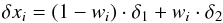 (74)where w is a smoothing function of the form
 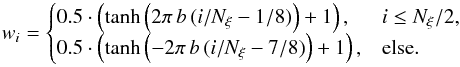 (75)The smoothing width b regulates by how much the cell width varies in the x direction. In the limit of b → ∞, one obtains a nonsmooth mapping with a discontinuity in the grid spacing in the x direction. The cell spacing in the y direction is kept constant for simplicity and is δy = Ly/Nη where Ly is the domain size in the y direction.
Parameters for the numerical setup differ slightly from those described in Sect. 4.3. In this section, the computational domain is [0,15] × [0,15] , and the center of the vortex is placed at (x0,y0) = (7.5,7.5). The boundary condition is periodic in both coordinate directions. All other parameters have the same values as in Sect. 4.3. We simulated the advection of this vortex for 15 time units, i.e., the vortex is advected across the computational domain once and returns to its initial position at the end of the simulations.
In Table 6 we give the order of convergence in dependence of the smoothing width b computed both in the L1 norm and the L∞ norm. For small values of b, we find fourth-order convergence, whereas for large b the results only show second-order convergence. For intermediate values of b, the convergence order changes from 2 to 4 when the resolution is increased. For a more quantitative discussion of the grid smoothness, we define the maximum expansion ratio 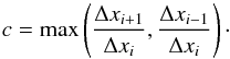 (76)As Table 7 shows there is a close correlation between the value of c and the L1 convergence rate; the numerical solution converges with fourth order when c ≲ 1.5 and with second order otherwise.
Dependence of the maximum expansion ratio of the grid c and the L1 convergence rate on the grid resolution and smoothing width b.
In accordance with the conclusions of Visbal & Gaitonde (2002) and Bassi & Rebay (1997), we find that the actually achievable order of high-order hydrodynamics codes depends on the grid smoothness, which can be assessed, amongst others, by the expansion ratio c (see the 1D example above) or the cell orthogonality (in multi-d applications). The latter is very poor for the grids proposed by Calhoun et al. (2008) and, hence, explains the poor performance of Apsara on these grids.
4.5. Gresho vortex
We considered the Gresho vortex problem (Gresho & Chan 1990) to test the capability of Apsara to treat low-Mach number flows. The Gresho vortex is a rotating flow in which the centrifugal forces are balanced by the pressure gradients, resulting in a steady-state solution of a rotating vortex. Miczek et al. (2015) used the Gresho vortex test to demonstrate the inability of Godunov-type schemes relying on Roe’s flux to correctly simulate low-Mach number flows. We follow their numerical setup here.
We simulated the flow in a 2D periodic domain [0,1] × [0,1] using the mapping M0. The fluid density ρ was set equal to 1 everywhere in the domain, and the vortex was placed at the center of the computational domain, i.e., the coordinates of its center were (x0,y0) = (0.5,0.5). The angular velocity of the rotating flow as a function of radius r measured from the center of the vortex is 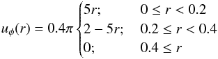 (77)and the radial profile of the fluid pressure is
 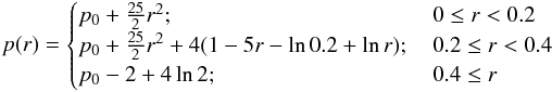 (78)with
 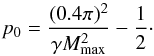 (79)The maximum Mach number Mmax of the rotating flow is attained at a radius r = 0.2. We used the ideal gas EOS with
  and evolved the vortex until time t = 1, i.e., until the vortex completed one revolution.
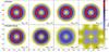 |
Fig. 3 Mach number distributions normalized by the maximum Mach number Mmax at t = 1 for the Gresho vortex test. The top and bottom rows show results computed by Apsara and Prometheus, respectively. Regardless of Mmax the vortex remains intact when simulated with Apsara, while with Prometheus the vortex gradually dissolves because of numerical dissipation as Mmax decreases. |
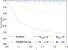 |
Fig. 4 Total kinetic energy as a function of time Ekin(t) normalized by the total kinetic of the initial state Ekin(0) for the Gresho vortex problem. The solid and dashed lines show the results computed with Apsara and Prometheus, respectively. Curves of different colors correspond to different maximum Mach numbers. In the case of Apsara, these curves are visually indistinguishable. |
Figure 3 shows the Mach number distributions at the final time t = 1 for decreasing values of Mmax ranging from 10-1 to 10-4. The results obtained with Apsara for different values of Mmax are almost identical, i.e., they are independent of Mmax. This behavior differs drastically from that found with Prometheus, for which the vortex gradually dissolves as Mmax decreases, and it eventually even disappears at Mmax = 10-4. The different performance of the two codes is also evident when one considers the time evolution of the total kinetic energy of the vortex, which is shown in Fig. 4 normalized by its initial value at t = 0. In the simulations performed with Apsara the total kinetic energy had decreased by less than 0.5% at t = 1 for all Mmax, while with Prometheus the vortex lost an increasingly larger amount of kinetic energy as Mmax was decreased. For Mmax = 10-4, more than half of the total kinetic energy was gone at the end of the simulation performed with Prometheus.
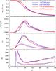 |
Fig. 5 Mean turbulent kinetic energy, mean dissipation rate of turbulent kinetic energy, mean enstrophy, and numerical Reynolds number (from top to bottom) plotted as function of the dimensionless time t∗ for the Taylor-Green vortex test for the reference Mach number Mref ~ 0.29. |
4.6. Taylor-Green vortex
We quantify the numerical viscosity of Apsara in the low-Mach number limit using the Taylor-Green vortex (Taylor & Green 1937) and compare it to Prometheus. Thereby, we follow the numerical setup described in Drikakis et al. (2007) and Edelmann (2014). The initial conditions were  where ρ0 = 1.178 × 10⁻³ g cm-3, p0 = 106 bar, and k = 0.01 cm-1. The velocity u0 was set by selecting a reference Mach number of the flow Mref = u0/c0, where
  is the sound speed. We considered two cases: Mref ~ 0.29 (i.e.u0 = 104 cm s-1) and Mref = 10-2. For both cases we used an ideal gas EOS with γ = 1.4. The vortex was simulated in a periodic cubic domain with an edge length of 2π·100 cm using the Cartesian mapping M0. The simulations were carried out with 643 and 1283 grid cells until a dimensionless time t∗ = ku0t = 30.
Figures 5 and 6 show a comparison of the results obtained with Apsara and Prometheus for simulations with Mref ~ 0.29 and Mref = 10-2, respectively. In both figures the top panel shows the time evolution of the nondimensionalized mean turbulent kinetic energy K∗ defined by  (85)where u = (u,v,w) is the velocity vector and the overbar denotes a volumetric average. As large-scale eddies decay to smaller ones, kinetic energy is dissipated by numerical viscosity. The corresponding energy dissipation rates are plotted in the second panels (from top) of Figs. 5 and 6, which show that the dissipation rate peaks roughly at the same time as the mean enstrophy,
  (86)given in the third panels of Figs. 5 and 6. From the enstrophy Ω∗ and the dissipation rate dK∗/ dt∗ we calculate the numerical Reynolds number Re using the relation
  (87)for an incompressible Navier-Stokes fluid (Drikakis et al. 2007). The numerical Reynolds number are plotted in the bottom panels of Figs. 5 and 6.
Although the results computed with Apsara and Prometheus do not differ markedly for Mref ~ 0.29 (Fig. 5), small differences can be recognized. The mean kinetic energy dissipates slightly faster near its peak for Prometheus than for Apsara for the same grid resolution. On the other hand, the mean enstrophy is slightly lower for Prometheus than for Apsara. As a consequence, the numerical Reynolds number is slightly higher for Apsara than for Prometheus, implying a lower numerical viscosity of the former code. This difference becomes more evident for Mref = 10-2 (Fig. 6); for a grid resolution of 1283 zones the Reynolds number is about 1.5 times larger for Apsara than for Prometheus.
Parameters used in our simulations to generate a turbulent flow (for more details see text).
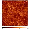 |
Fig. 7 Square root of the magnitude of the vorticity |
5. Turbulence in the context of core collapse supernovae
Lately, the study of the properties of turbulent flows in CCSN has received great attention among supernova researchers because turbulent pressure is thought to provide additional support for the revival of the stalled supernova shock wave, thus aiding an explosion (Murphy et al. 2013; Couch & Ott 2015). Abdikamalov et al. (2015) investigated the resolving power of 3D CCSN simulations. They concluded that the grid resolutions presently used in 3D implicit large eddy simulations (ILES) of CCSN are still at least ~7−8 times too low to correctly model the turbulent energy cascade down to the inertial range. Instead, the excessive numerical viscosity resulting from a grid resolution that is too low causes inefficient transport of kinetic energy from large to small scales, creating a pile-up of energy between the energy injection scale and the dissipation range. Their conclusion concerning a grid resolution that is adequate for resolving the inertial range is based on earlier work on isotropic, stationary turbulence by Sytine et al. (2000). However, because turbulence in CCSN is driven by time-dependent neutrino heating of post-shock matter, the resulting turbulent flow is anisotropic and nonstationary.
To study turbulence in the regime relevant to CCSN Radice et al. (2015) performed simulations of anisotropic turbulence with a characteristic Mach number of ~0.3 in a 3D Cartesian box using the Flash code (Fryxell et al. 2000; Dubey et al. 2009). In their simulations, the stirring force is enhanced in the x direction, which they used to mimic the preferred radial direction in CCSN, such that the turbulent kinetic energy is twice larger in the x direction than in the other two coordinate directions. They considered five different HRSC methods varying the spatial reconstruction order, Riemann solver, and grid resolutions. Their findings agree with those of the previous study by Sytine et al. (2000) of isotropic turbulence. At low resolution, the energy cascade is strongly affected by the bottleneck effect. Radice et al. (2015) recovered the inertial range only partially even at the highest resolution (512 grid points per coordinate direction) considered. These authors estimated that at this resolution about 20% of the energy is still accumulated at intermediate scales using the least dissipative scheme considered in their work.
Motivated by the study of Radice et al. (2015) we performed a set of ILES of anisotropic turbulence in the context of CCSN with Apsara. Our numerical setup resembles that of Radice et al. (2015) and can be summarized as follows. Turbulence is driven by an external acceleration field by adding a stirring acceleration term to the RHS of the momentum equation. We closely followed the implementation of the stirring module in Flash and list the respective parameters in Table 8. We generated an acceleration field that was purely solenoidal (divergence-free), only containing power within a small range of Fourier modes between wavenumbers kmin and kmax. Six separate phases are evolved for each stirring mode after each time step Δt in Fourier space by an Ornstein-Uhlenbeck (OU) random process (Uhlenbeck & Ornstein 1930). The phases ψ are updated as 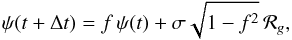 (88)where f = exp(−Δt/τ) is a decay factor with correlation timescale τ, and σ is the variance of the OU process. The value ℛg is a Gaussian random variable drawn from a Gaussian distribution with unit variance. The power per mode is set by the variance σ and is chosen to be constant for all excited wavenumbers. To break isotropy, we multiplied the OU variance σ in x direction by a factor of four before carrying out the solenoidal projection in Fourier space. We tuned the OU variance σ such that the flow has a rms Mach number of ≈0.37.
We performed the simulations in a unit cube using the Cartesian mapping M0 employing four grid resolutions of 643, 1283, 2563, and 5123 zones, respectively. We simulated the evolution of the flow until t = 100. Figure 7 shows a snapshot at the final time of the square root of the magnitude of the vorticity  in a 2D (x-z) slice through the middle of the simulation box (y = 0) for the simulation with 5123 zones. In Fig. 8 we show for all grid resolutions the compensated 1D energy spectra E(k) k5/3, which we computed following Radice et al. (2015).
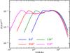 |
Fig. 8 Energy spectra (Eq. (89)) plotted vs. the dimensionless wavenumber 512kΔx for four different grid resolutions. The spectra are compensated by a k5/3 spectrum, so that any region with Kolmogorov scaling appears flat. |
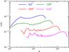 |
Fig. 9 Effective numerical viscosity (Eq. (91)) as a function of wavenumber estimated from our ILES simulations for four different grid resolutions. |
We computed first the 3D energy spectrum  (89)where
  is the Fourier transform of the velocity field and
  is its complex conjugate. To obtain the 1D energy spectrum E(k), we averaged the 3D spectrum over spherical shells in k space (Eswaran & Pope 1988)
  (90)where Nk denotes the number of discrete modes within the bin
  . We then averaged E(k) over time using 381 snapshots in the interval 5 ≤ t ≤ 100 spaced by 0.25 time units.
The resulting energy spectra are in very good agreement with those of the least dissipative numerical schemes considered by Radice et al. (2015), i.e., the third-order PPM reconstruction (Colella & Woodward 1984) and the improved fifth-order WENO reconstruction (WENO-Z; Borges et al. 2008) using the HLLC approximate Riemann solver of Toro et al. (1994). The compensated spectrum exhibits a flat region with Kolmogorov scaling (for 5 ≲ k ≲ 10) expected in the inertial range only at a resolution of 5123. At lower grid resolutions the compensated energy spectra are dominated by the bottleneck effect, which manifests itself with a ~k-1 scaling.
On the other hand, the effective viscosity measured from our simulations differs from that reported in Radice et al. (2015). It is estimated according to  (91)where
 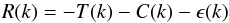 (92)is the residual of the 1D energy balance equation. The 1D energy transfer term T(k),C(k), and the energy injection rate ϵ(k) are averages of their 3D counterparts T(k),C(k), and ϵ(k), and are obtained in the same way we calculated the 1D energy spectrum E(k) (Eq. (90)). The 3D counterparts are defined as
 ![\begin{eqnarray} &&T(\bs{k}) = 2\pi\, \Re[(\hat{\bs{u}}*i\bs{k} \otimes \hat{\bs{u}})\cdot\hat{\bs{u}}^*], \label{eq:Tterm}\\ &&C(\bs{k}) = 2\pi\, \Re[(\frac{1}{\rho}*i\bs{k}p)\cdot\hat{\bs{u}}^*], \label{eq:Cterm}\\ &&\epsilon(\bs{k}) = \Re[\hat{\bs{a}}\cdot\hat{\bs{u}}^*], \end{eqnarray}](/articles/aa/full_html/2016/11/aa28205-16/aa28205-16-eq343.png) where
where  is the Fourier transform of the acceleration field and ∗ denotes the convolution operator. In Fig. 9 we show the effective numerical viscosity ν(k) as a function of wavenumber estimated from our simulations. The effective viscosity exhibits fewer variations in k space than that estimated by Radice et al. (2015) from their simulations (see their Fig. 5).
6. Summary
We have developed a new numerical code for simulating astrophysical flows called Apsara. The code is based on the fourth-order implementation of a high-order, finite-volume method for mapped coordinates proposed by Colella et al. (2011). An extension of the method for solving nonlinear hyperbolic equations following McCorquodale & Colella (2011) and Guzik et al. (2012) is applied to solve the Euler equations of Newtonian gas dynamics. Apsara comprises great flexibility concerning grid geometry because of the implemented mapped-grid technique, which makes the code suitable for a wide range of applications.
By defining a mapping function, which describes the coordinate transformation between physical space and an abstract computational space, the governing equations written in Cartesian coordinates in physical space are transformed into equations of similar form in the computational space. The physical domain of interest can then be discretized as a general structured curvilinear mesh, while the computational space is still discretized by an equidistant Cartesian mesh that allows for easy and efficient implementation of numerical algorithms.
We strictly follow the implementation described in Colella et al. (2011) for computation of metric terms on faces of control volumes to ensure that Apsara preserves the freestream condition. The freestream property is crucial for grid-based codes in curvilinear coordinates because violation of this condition can introduce numerical artifacts as shown, for example, in Grimm-Strele et al. (2014) for the WENO-G finite difference scheme (Nonomura et al. 2010; Shu 2003).
The method of Colella et al. (2011) can be extended to a higher order of accuracy in time as described in Buchmüller & Helzel (2014). However, RK schemes of order higher than four are considerably more expensive because many more integration stages are needed in this case (Ketcheson 2008). Concerning fourth-order accurate RK schemes, the ten-stage algorithm SSPRK(10, 4) of Ketcheson (2008) has the advantage of possessing the strong stability-preserving (SSP) property, which is not the case for the classical RK4 scheme. In this work, however, we always used the RK4 scheme and the extension to the SSPRK(10, 4) scheme is subject of the future development of Apsara.
We validated our numerical code by simulating a set of hydrodynamic tests problems. In the case of smooth solutions, i.e., for the linear advection of a Gaussian profile, the propagation of a linear acoustic wave, and the advection of a nonlinear vortex, Apsara exhibits fourth-order accuracy both on a Cartesian mesh and the sinusoidally deformed mesh considered by Colella et al. (2011). However, our results from the advection of a nonlinear vortex test also revealed that the order of accuracy is severely degraded when using the circular mapping proposed by Calhoun et al. (2008), i.e., the grid smoothness directly impacts the achievable order of accuracy of the scheme. Our finding agrees with results obtained by Lemoine & Ou (2014), who used a modified version of grid mappings suggested by Calhoun et al. (2008). Lemoine & Ou also achieved roughly first-order convergence on these nonsmooth grid mappings. Thus, we conclude that the singularity-free mappings for circular and spherical domains of Calhoun et al. (2008) are not suitable for use in conjuction with high-order, finite-volume methods.
We quantified how the grid smoothness influences the order of accuracy of the high-order method of Colella et al. (2011) using the advection of a nonlinear vortex across a 2D mesh varying the nonequidistant grid spacing in one coordinate direction systematically. We found that the grid expansion ratio, i.e., the ratio of the cell size between two neighboring zones, must be less than ~1.5 in order to preserve fourth-order accuracy. This result can be regarded as a guideline for the grid setup in the case of a logarithmically spaced radial grid that is often employed in astrophysical simulations in spherical geometry.
Motivated by the work of Miczek et al. (2015), which demonstrated a failure of a Godunov-type scheme employing a Roe flux in the low-Mach number regime, we performed simulations of the Gresho vortex test varying the maximum Mach number of the vortex from 10-1 to 10-4. Our results show that the decrease of the kinetic energy of the vortex is independent of the maximum Mach number when computed with Apsara. In all our simulations the kinetic energy had decreased by less than ≈0.5% at the end of the simulations, i.e., after one complete rotation of the vortex. This contrasts with solutions calculated with Prometheus, which uses the dimensionally-split PPM method as do many other codes in astrophysics. The kinetic energy of the vortex decreased more and more rapidly when the maximum Mach number was decreased. In the lowest Mach number case, the Gresho vortex vanished completely and the kinetic energy was reduced by more than half of its initial value because of the numerical dissipation present in Prometheus.
The superior performance of the high-order method of McCorquodale & Colella (2011) for highly subsonic flows is further supported by our results obtained for the Taylor-Green vortex problem. We simulated this test for two reference Mach numbers and compared the results computed with Apsara and Prometheus. For a reference Mach number 0.29 we obtained similar results for both codes, whereas, for a reference Mach number 10-2, Apsara achieved a larger numerical Reynolds number for the same resolution, implying a lower numerical viscosity than Prometheus.
To demonstrate Apsara’s performance on an astrophysical application, we performed ILES of anisotropic turbulence in a periodic Cartesian domain following the numerical setup used by Radice et al. (2015). The characteristic Mach number of the flow was 0.37, and the acceleration field driving the turbulence was enhanced along one coordinate direction to mimic the turbulent flow conditions in a CCSN. We obtained very similar results as those reported by Radice et al. (2015). At low resolution the energy spectra are dominated by the bottleneck effect at intermediate scales. We only began to recover the inertial range for a narrow range of wavenumbers at the highest grid resolution of 512 zones per coordinate direction. On the other hand, the effective viscosity as a function of wavenumber displayed fewer variations than that of Radice et al. (2015).
For problems to be simulated in a spherical domain, which we are particularly interested in, the singularity-free grid mappings of Calhoun et al. (2008) result in a loss of convergence order. Therefore, we plan to implement the mapped multiblock grid technique into Apsara following the strategy of McCorquodale et al. (2015), who extended the high-order, finite-volume method of Colella et al. (2011) to include this technique. They described an algorithm for data communication between blocks such that high-order accuracy is maintained. We also plan to implement additional physics into Apsara, for example, self-gravity, a nuclear EOS, and a nuclear reaction network, to tackle multiphysics astrophysical problems such as CCSN and stellar convection.
Acknowledgments
Most of the computations were performed at the Max Planck Computing & Data Facility (MPCDF). A.W. thanks Tomoya Takiwaki for fruitful discussions on turbulence in CCSN and H.G.S. acknowledges financial support from the Austrian Science fund (FWF), project P21742.
References
- Abdikamalov, E., Ott, C. D., Radice, D., et al. 2015, ApJ, 808, 70 [NASA ADS] [CrossRef] [Google Scholar]
- Appel, W. 2007, Mathematics for Physics and Physicists (Princeton University Press) [Google Scholar]
- Bassi, F., & Rebay, S. 1997, J. Comput. Phys., 138, 251 [Google Scholar]
- Borges, R., Carmona, M., Costa, B., & Don, W. S. 2008, J. Comput. Phys., 227, 3191 [Google Scholar]
- Buchmüller, P., & Helzel, C. 2014, J. Sci. Comput., 61, 343 [CrossRef] [Google Scholar]
- Calhoun, D. A., Helzel, C., & Leveque, R. J. 2008, SIAM Rev., 50, 723 [CrossRef] [Google Scholar]
- Cardall, C. Y., Budiardja, R. D., Endeve, E., & Mezzacappa, A. 2014, ApJS, 210, 17 [NASA ADS] [CrossRef] [Google Scholar]
- Colella, P., & Glaz, H. M. 1985, J. Comput. Phys., 59, 264 [NASA ADS] [CrossRef] [Google Scholar]
- Colella, P., & Sekora, M. D. 2008, J. Comput. Phys., 227, 7069 [NASA ADS] [CrossRef] [Google Scholar]
- Colella, P., & Woodward, P. R. 1984, J. Comput. Phys., 54, 174 [NASA ADS] [CrossRef] [MathSciNet] [Google Scholar]
- Colella, P., Dorr, M. R., Hittinger, J. A. F., & Martin, D. F. 2011, J. Comput. Phys., 230, 2952 [NASA ADS] [CrossRef] [EDP Sciences] [Google Scholar]
- Couch, S. M., & Ott, C. D. 2015, ApJ, 799, 5 [NASA ADS] [CrossRef] [Google Scholar]
- Drikakis, D., Fureby, C., Grinstein, F. F., & Youngs, D. 2007, J. Turbulence, 8, N20 [CrossRef] [Google Scholar]
- Dubey, A., Antypas, K., Ganapathy, M. K., et al. 2009, Parallel Computing, 35, 512 [CrossRef] [Google Scholar]
- Edelmann, P. 2014, Dissertation, Technische Universität München, München [Google Scholar]
- Eswaran, V., & Pope, S. B. 1988, Computers and Fluids, 16, 257 [NASA ADS] [CrossRef] [Google Scholar]
- Feng, X., Jiang, C., Xiang, C., Zhao, X., & Wu, S. T. 2012, ApJ, 758, 62 [Google Scholar]
- Fragile, P. C., Lindner, C. C., Anninos, P., & Salmonson, J. D. 2009, ApJ, 691, 482 [NASA ADS] [CrossRef] [Google Scholar]
- Fryxell, B., Arnett, D., & Mueller, E. 1991, ApJ, 367, 619 [NASA ADS] [CrossRef] [Google Scholar]
- Fryxell, B., Olson, K., Ricker, P., et al. 2000, ApJS, 131, 273 [NASA ADS] [CrossRef] [Google Scholar]
- Gresho, P. M., & Chan, S. T. 1990, Int. J. Numer. Meth. Fluids, 11, 621 [Google Scholar]
- Grimm-Strele, H., Kupka, F., & Muthsam, H. J. 2014, Comput. Phys. Comm., 185, 764 [Google Scholar]
- Guzik, S., McCorquodale, P., & Colella, P. 2012, in 50th AIAA Aerospace Sciences Meetings (American Institute of Aeronautics and Astronautics, Nashville, TN), AIAA Paper 2012–0574 [Google Scholar]
- Hayashi, H., & Kageyama, A. 2016, J. Comput. Phys., 305, 895 [NASA ADS] [CrossRef] [Google Scholar]
- Hotta, H., Rempel, M., & Yokoyama, T. 2014, ApJ, 786, 24 [NASA ADS] [CrossRef] [Google Scholar]
- Jiang, C., Feng, X., & Xiang, C. 2012, ApJ, 755, 62 [NASA ADS] [CrossRef] [Google Scholar]
- Kageyama, A., & Sato, T. 2004, Geophys., Geosys., 5, 9005 [Google Scholar]
- Ketcheson, D. I. 2008, SIAM J. Sci. Comput., 30, 2113 [CrossRef] [Google Scholar]
- Kifonidis, K., & Müller, E. 2012, A&A, 544, A47 [NASA ADS] [CrossRef] [EDP Sciences] [Google Scholar]
- Koldoba, A. V., Romanova, M. M., Ustyugova, G. V., & Lovelace, R. V. E. 2002, ApJ, 576, L53 [NASA ADS] [CrossRef] [Google Scholar]
- Lemoine, G. I., & Ou, M. Y. 2014, SIAM J. Sci. Comput., 36, B396 [CrossRef] [Google Scholar]
- Lentz, E. J., Bruenn, S. W., Hix, W. R., et al. 2015, ApJ, 807, L31 [NASA ADS] [CrossRef] [Google Scholar]
- LeVeque, R. 2002, Finite Volume Methods for Hyperbolic Problems, Cambridge Texts in Applied Mathematics (Cambridge University Press) [Google Scholar]
- McCorquodale, P., & Colella, P. 2011, CAMCOS, 6, 1 [CrossRef] [Google Scholar]
- McCorquodale, P., Dorr, M. R., Hittinger, J. A. F., & Colella, P. 2015, J. Comput. Phys., 288, 181 [NASA ADS] [CrossRef] [Google Scholar]
- Melson, T., Janka, H.-T., Bollig, R., et al. 2015a, ApJ, 808, L42 [NASA ADS] [CrossRef] [Google Scholar]
- Melson, T., Janka, H.-T., & Marek, A. 2015b, ApJ, 801, L24 [NASA ADS] [CrossRef] [Google Scholar]
- Miczek, F., Röpke, F. K., & Edelmann, P. V. F. 2015, A&A, 576, A50 [NASA ADS] [CrossRef] [EDP Sciences] [Google Scholar]
- Mueller, E., Fryxell, B., & Arnett, D. 1991, A&A, 251, 505 [NASA ADS] [Google Scholar]
- Müller, B. 2015, MNRAS, 453, 287 [NASA ADS] [CrossRef] [Google Scholar]
- Murphy, J. W., Dolence, J. C., & Burrows, A. 2013, ApJ, 771, 52 [NASA ADS] [CrossRef] [Google Scholar]
- Nonomura, T., Iizuka, N., & Fujii, K. 2010, Computers & Fluids, 39, 197 [CrossRef] [Google Scholar]
- Peng, X., Xiao, F., & Takahashi, K. 2006, Quart. J. Roy. Meteor. Soc., 132, 979 [NASA ADS] [CrossRef] [Google Scholar]
- Radice, D., Couch, S. M., & Ott, C. D. 2015, Comput. Astrophys. Cosmol., 2, 7 [NASA ADS] [CrossRef] [Google Scholar]
- Romanova, M. M., Ustyugova, G. V., Koldoba, A. V., & Lovelace, R. V. E. 2012, MNRAS, 421, 63 [NASA ADS] [Google Scholar]
- Ronchi, C., Iacono, R., & Paolucci, P. S. 1996, J. Comput. Phys., 124, 93 [NASA ADS] [CrossRef] [MathSciNet] [Google Scholar]
- Shiota, D., Kusano, K., Miyoshi, T., & Shibata, K. 2010, ApJ, 718, 1305 [NASA ADS] [CrossRef] [Google Scholar]
- Shu, C.-W. 2003, Int. J. Comput. Fluid Dyn., 17, 107 [NASA ADS] [CrossRef] [Google Scholar]
- Stone, J. M., Gardiner, T. A., Teuben, P., Hawley, J. F., & Simon, J. B. 2008, ApJS, 178, 137 [NASA ADS] [CrossRef] [Google Scholar]
- Sytine, I. V., Porter, D. H., Woodward, P. R., Hodson, S. W., & Winkler, K.-H. 2000, J. Comput. Phys., 158, 225 [NASA ADS] [CrossRef] [Google Scholar]
- Taylor, G. I., & Green, A. E. 1937, Proc. Roy. Soc. London A, 158, 499 [Google Scholar]
- Toro, E. F., Spruce, M., & Speares, W. 1994, Shock Waves, 4, 25 [NASA ADS] [CrossRef] [EDP Sciences] [Google Scholar]
- Uhlenbeck, G. E., & Ornstein, L. S. 1930, Phys. Rev., 36, 823 [NASA ADS] [CrossRef] [Google Scholar]
- Visbal, M. R., & Gaitonde, D. V. 2002, J. Comput. Phys., 181, 155 [NASA ADS] [CrossRef] [Google Scholar]
- Warren, D. C., & Blondin, J. M. 2013, MNRAS, 429, 3099 [NASA ADS] [CrossRef] [Google Scholar]
- Wilson, J. R., & Mayle, R. W. 1988, Phys. Rep., 163, 63 [NASA ADS] [CrossRef] [Google Scholar]
- Wongwathanarat, A., Hammer, N. J., & Müller, E. 2010, A&A, 514, A48 [NASA ADS] [CrossRef] [EDP Sciences] [Google Scholar]
- Wongwathanarat, A., Müller, E., & Janka, H.-T. 2015, A&A, 577, A48 [NASA ADS] [CrossRef] [EDP Sciences] [Google Scholar]
- Yee, H. C., Vinokur, M., & Djomehri, M. J. 2000, J. Comput. Phys., 162, 33 [NASA ADS] [CrossRef] [Google Scholar]
Appendix A: Coarse-fine interpolation
We consider a coarse grid and a fine grid in 1D, which is refined from the coarse grid by a factor of two, i.e., fine grid cells i and i + 1 are the subdivisions of the coarse grid cell i′. To compute a fourth-order accurate approximation of a scalar quantity  at a cell center of a zone i′ on the coarse grid from cell averages ⟨ qf ⟩ on the fine grid, we expand q with respect to the cell center of the coarse grid as
  (A.1)Integrating this equation to obtain cell averages ⟨ qf ⟩ for the zones i−1, i, i + 1 and i + 2 yields a system of equations
 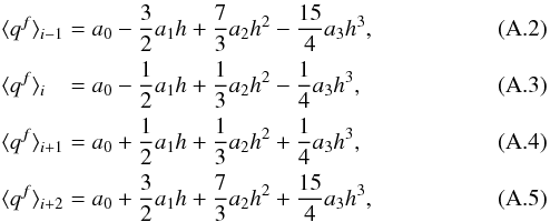 where h is the cell spacing on the fine grid. Solving this system of equations for a0 gives
 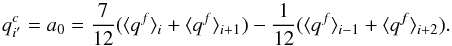 (A.6)The same procedure can be applied in a straightforward manner in 2D and 3D. The respective expressions for the 2D case read
 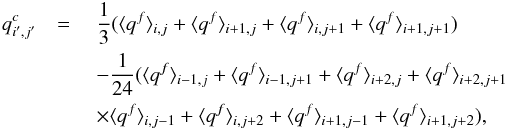 (A.7)
(A.7)
All Tables
L1 and L∞ errors of ⟨ ρ ⟩, and the convergence rates for the 1D linear advection test.
L1-norm of the coarse-fine differences of the pointwise densities ρ as a function of grid resolution for the linear acoustic wave test.
L1 and L∞ errors of ρ, and their convergence rates for the 2D advection of a nonlinear vortex test.
Dependence of the maximum expansion ratio of the grid c and the L1 convergence rate on the grid resolution and smoothing width b.
Parameters used in our simulations to generate a turbulent flow (for more details see text).
All Figures
|
Fig. 1 Examples of 2D meshes generated using smooth mapping M1 (left) and circular mapping M2 (right). |
| In the text | |
|
Fig. 2 Density profiles for the 1D linear advection test obtained on a grid of 128 zones at t = 10. Results computed with Apsara and Prometheus are shown with blue crosses and red circles, respectively. The exact solution is shown in black. |
| In the text | |
|
Fig. 3 Mach number distributions normalized by the maximum Mach number Mmax at t = 1 for the Gresho vortex test. The top and bottom rows show results computed by Apsara and Prometheus, respectively. Regardless of Mmax the vortex remains intact when simulated with Apsara, while with Prometheus the vortex gradually dissolves because of numerical dissipation as Mmax decreases. |
| In the text | |
|
Fig. 4 Total kinetic energy as a function of time Ekin(t) normalized by the total kinetic of the initial state Ekin(0) for the Gresho vortex problem. The solid and dashed lines show the results computed with Apsara and Prometheus, respectively. Curves of different colors correspond to different maximum Mach numbers. In the case of Apsara, these curves are visually indistinguishable. |
| In the text | |
|
Fig. 5 Mean turbulent kinetic energy, mean dissipation rate of turbulent kinetic energy, mean enstrophy, and numerical Reynolds number (from top to bottom) plotted as function of the dimensionless time t∗ for the Taylor-Green vortex test for the reference Mach number Mref ~ 0.29. |
| In the text | |
 |
Fig. 6 Same as Fig. 5, but for Mref = 10-2. |
| In the text | |
|
Fig. 7 Square root of the magnitude of the vorticity |
| In the text | |
|
Fig. 8 Energy spectra (Eq. (89)) plotted vs. the dimensionless wavenumber 512kΔx for four different grid resolutions. The spectra are compensated by a k5/3 spectrum, so that any region with Kolmogorov scaling appears flat. |
| In the text | |
|
Fig. 9 Effective numerical viscosity (Eq. (91)) as a function of wavenumber estimated from our ILES simulations for four different grid resolutions. |
| In the text | |
Current usage metrics show cumulative count of Article Views (full-text article views including HTML views, PDF and ePub downloads, according to the available data) and Abstracts Views on Vision4Press platform.
Data correspond to usage on the plateform after 2015. The current usage metrics is available 48-96 hours after online publication and is updated daily on week days.
Initial download of the metrics may take a while.