| Issue |
A&A
Volume 594, October 2016
|
|
|---|---|---|
| Article Number | A41 | |
| Number of page(s) | 7 | |
| Section | Stellar atmospheres | |
| DOI | https://doi.org/10.1051/0004-6361/201628491 | |
| Published online | 07 October 2016 | |
Glimpses of stellar surfaces
I. Spot evolution and differential rotation of the planet host star Kepler-210
Hamburger Sternwarte, Universität Hamburg, Gojenbergsweg 112, 21029 Hamburg, Germany
e-mail: This email address is being protected from spambots. You need JavaScript enabled to view it.
Received: 11 March 2016
Accepted: 25 May 2016
Abstract
We use high accuracy photometric data obtained with the Kepler satellite to monitor the activity modulations of the Kepler-210 planet host star over a time span of more than four years. Following the phenomenology of the star’s light curve in combination with a five spot model, we identify six different so-called spot seasons. A characteristic, which is common in the majority of the seasons, is the persistent appearance of spots in a specific range of longitudes on the stellar surface. The most prominent period of the observed activity modulations is different for each season and appears to evolve following a specific pattern, resembling the changes in the sunspot periods during the solar magnetic cycle. Under the hypothesis that the star exhibits solar-like differential rotation, we suggest differential rotation values of Kepler-210 that are similar to or smaller than that of the Sun. Finally, we estimate spot life times between ~60 days and ~90 days, taking into consideration the evolution of the total covered stellar surface computed from our model.
Key words: stars: activity / starspots / stars: rotation
© ESO, 2016
1. Introduction
The nature of the magnetic dynamo and the role of differential rotation in dwarf main-sequence stars is not yet fully understood. While these types of stars often exhibit substantial photometric variability, the amplitude of their surface differential rotation is expected to be small (Küker & Rüdiger 2008). The inability of the small or absent differential rotation to organize the global magnetic field of those stars may result in the absence of activity cycles as observed in the Sun (Chabrier & Küker 2006). As a result, the study of photospherically active stars and the measurement of their differential rotation rates is an important piece of information for all dynamo theories.
The rotational periods of stars can be measured with a variety of techniques including monitoring of the intensity variations of the cores of the Ca H+K lines, spectral line broadening (for cases with known stellar radius and inclination), and the analysis of pseudo-periodic photometric modulations as a result of surface inhomogeneities in the form of photospheric activity (spots). The successful operation of the space missions CoRoT (Baglin et al. 2006) and Kepler (Borucki et al. 2010), in combination with their high photometric accuracy and long, non-interrupted observations has revolutionized the studies of stellar rotation with period measurements being available for a very large number of field stars (Reinhold et al. 2013; McQuillan et al. 2014). Furthermore, the analysis of the photometric light curves of CoRoT and Kepler, using a variety of techniques, including power spectrum analysis (Reinhold & Reiners 2013) and spot modeling (Fröhlich et al. 2009; Huber et al. 2009; Frasca et al. 2011; Bonomo & Lanza 2012), makes it possible to measure the stellar differential rotation and other physical characteristics of star spots.
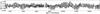 |
Fig. 1 Complete light curve of the Kepler-210 (~1400 days), normalized and with the planetary transits excluded (see text for details). |
In this paper we use the light curve phenomenology of Kepler-210 (i.e., the variations of the light curve between the stellar rotations) in combination with spot modeling and power spectrum analysis to study its photospheric activity. In the first part of Sect. 2 we describe the data and the properties of Kepler-210. In the second part of this section we present the details of the spot model used in our analysis and explain our choices regarding the number of free parameters in our model. In Sect. 3, we show the results of our combined analysis and, in Sect. 4, we attempt to provide a physical interpretation of our results. Finally, we conclude with a summary in Sect. 5.
2. Data and analysis
2.1. Light curve and periodogram
The Kepler-210 system consists of a K dwarf with at least two planets orbiting around it (Ioannidis et al. 2014). The Kepler light curve of the system was obtained from the STDADS1 archive and contains the long cadence data from quarters Q1 to Q17. The removal of instrumental systematics from the Kepler light curves is quite cumbersome (Petigura & Marcy 2012; McQuillan et al. 2012; Kinemuchi et al. 2012), thus we decided to use the so-called corrected PDC-MAP data for our analysis. Stumpe et al. (2012) provide a detailed description of the philosophy behind the PDC-MAP approach and, in our study we rely on the ability of this algorithm to remove instrumental effects, but to retain astrophysical effects. In Fig. 1, we show the approximately 1400 days long light curve of Kepler-210 with each quarter normalized by its mean and the planetary transits removed (using the parameters calculated by Ioannidis et al. 2014). The light curve shows clear modulations with an amplitude of ~2%, similar to photospherically active stars, e.g., CoRoT-2 (cf., Alonso et al. 2008; Huber et al. 2009). To analyze those modulations we use the generalized Lomb-Scargle (L-S) periodogram (Zechmeister & Kürster 2009) of the total light curve of Kepler-210. The peak with the highest power corresponds to a period of P⋆ = 12.28 days (see, Sect. 3.2). However, we find evidence for additional power on various timescales which we would like to explore in the following.
2.2. Light curve modeling
2.2.1. Basics
To describe the relative stellar flux reduction Fsp/F0, which is due to the presence of an active region on the stellar surface, we adopt a simple spot model, given by the expression ![Mathematical equation: \begin{eqnarray} \nonumber \label{eq:spotflux} \frac{F_\mathrm{sp}}{F_0} &=& 1 - \frac{S_\mathrm{sp} \cdot \cos[\, \theta(t)]}{\pi R_{\star}^{2}} \,\\ &&\times ( 1 - t_\mathrm{sp}^4 )\cdot I[\, \theta(t)\, ,c_1,c_2] . \end{eqnarray}](/articles/aa/full_html/2016/10/aa28491-16/aa28491-16-eq4.png) (1)The terms Ssp, R⋆, and tsp denote the spotted surface, the stellar radius, and the relative spot temperature (i.e., the ratio between spot temperature and photospheric temperature) respectively. The term θ(t) accounts for the angle between the line of sight towards the observer and the normal to the spotted surface at the time t of the observation. The factor I [ θ(t),c1,c2 ] denotes the limb darkening (LD) of the stellar disk, which depends on the angle θ(t). We use a quadratic LD parameterization, with the parameters c1 and c2 as limb-darkening coefficients (LDC).
(1)The terms Ssp, R⋆, and tsp denote the spotted surface, the stellar radius, and the relative spot temperature (i.e., the ratio between spot temperature and photospheric temperature) respectively. The term θ(t) accounts for the angle between the line of sight towards the observer and the normal to the spotted surface at the time t of the observation. The factor I [ θ(t),c1,c2 ] denotes the limb darkening (LD) of the stellar disk, which depends on the angle θ(t). We use a quadratic LD parameterization, with the parameters c1 and c2 as limb-darkening coefficients (LDC).
For simplicity, we assume dark circular spots (tsp = 0) and note that the spot temperature can be calibrated later by increasing the values of the spot radius (see discussion in Sect. 2.2.2). Owing to the fact that Kepler-210 hosts a planetary system, we feel secure in assuming that the stellar inclination is ≃90° (Tremaine & Dong 2012; Figueira et al. 2012; Johansen et al. 2012; Fang & Margot 2012; Fabrycky et al. 2014; Morton & Winn 2014); which we adopt in the following.
2.2.2. Spot modeling
In our modeling, we assume purely equatorial spots since the latitude of an active region on the star can be regulated by its size Ssp, while the term θ(t) can be used to express the longitude of the region during the observation; λo = 0° stands for the sub-observer point at the center of disk, with λo = −90° being the leading edge, and λo = 90° the trailing edge of the disk.
To study the validity of this adopted equatorial spot model, we consider noise-free light curves of fiducial spotted stars with various inclinations, where spots of some given size (we chose Rsp/R⋆ = 0.1) are placed at various stellar latitudes. The calculated light curves are fitted with an equatorial spot model, i.e., the spot latitude is set to zero, but the size of the spot is allowed to vary. We then compute the maximal (absolute) deviation (in amplitude) between the true light curve and the light curve modeled with equatorial spots and plot, in Fig. 2, this maximal deviation as a function of spot latitude for various inclinations. As can be seen from Fig. 2, these deviations disappear for latitudes of zero (where the spots are already on the equator) and for polar spots, which produce essentially no rotational modulations. The largest deviations occur for spots at latitudes between 30°−60° placed on stars seen with inclinations between 10°−70°. In those cases the visibility duration of a spot does depend on latitude, while for inclinations near 90° all spots have essentially the same visibility duration and spots at different latitudes differ only through the effects of differential LD.
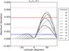 |
Fig. 2 Amplitude of the simulated light curves residuals after the subtraction of the fitted equatorial spot model. The red lines show the mean variation of the modulations from one rotation to the next (solid red line) and its uncertainty (dashed red lines). The blue solid line represents the level of the Gaussian noise of the Kepler-210 light curve. |
In Fig. 2 we also indicate the typical noise in the Kepler data of Kepler-210 (solid blue line) as well as the observed mean peak to peak variation (solid red line) and its dispersion (dashed red lines). Figure 2 then indicates that, for inclinations in excess of about 70°, the noise in the data exceeds the maximally possible deviations introduced by the equatorial spot model. Since we assume an inclination close to 90° for Kepler-210, we argue that our modeling approach with only equatorial spots is in order and that reliable latitude information cannot be retrieved from the light curve.
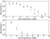 |
Fig. 3 χ2 goodness of the fit for models with different number of equally separated spots (upper panel) and free spots (lower panel). It is clear that the normalized χ2 is approaching close to unity for models with at least 10 free parameters (see text for details). |
2.2.3. Light curve modeling
To describe the observed light curve changes, we consider chunks of the overall light curve (see Fig. 1), equal to the leading period of the L-S periodogram, separated by a quarter of that period, i.e., the individual light curves are not independent. The light curve modulations are not sufficiently stable from one rotation to the next, so none of the light curve chunks are identical. To cope with this problem we use equatorial spot models to describe the observed modulations. Each spot model then represents a unique passage of this region over the visible hemisphere of the star.
It is well known that the problem of modeling the spot distribution on a two-dimensional surface into a one-dimensional light curve is ill-posed, i.e., in general there is more than one model to appropriately describe the observed light curve modulations. For our light curve modeling, we consider two different approaches: in the first approach, we consider N circular dark spots, where the ith spot has a radius Ri and is located on the equator at some longitude λi; as a second approach, we again consider N circular dark spots, this time however, at fixed, equidistant locations around the stellar equator. Since the star appears to always be covered by spots and since stitching of the individual quarters may not be fully correct, it is impossible to know the correct normalization of the light curve. As a result, we include an estimate of the level of the unspotted flux in our model. To assess the goodness of fit, we compute the χ2-values of our fit for all models. Although the quality of the model fits increases with the number of spots, i.e., the number of the available free parameters, this number should be as low as necessary. Therefore we first address the question of the effective number of free parameters in our problem.
In the upper panel of Fig. 3, we first consider the χ2-values for models with a given number of fixed spots at equidistant locations around the equator for three randomly chosen light curve chunks (described by different symbols). As the spots are described by only one free parameter (their respective radius), the number of spots is equal to the number of free parameters of the model plus one (for the normalization factor). It is clear that around ten such spots are required to obtain acceptable fits.
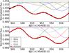 |
Fig. 4 Top: visual representation of the 10 fixed spot model. Each of the thin colored lines represents the flux reduction caused from each of the spots during a full rotation. The combined flux reduction is given from the aggregation of the five spots models (thick red line). Bottom: as for top panel, but for the five-spot model. |
In the lower panel of Fig. 3 we consider models with a variable number of spots at variable positions along the equator and plot again the χ2-values as a function of spot number. Clearly, Fig. 3 suggests that one needs about five free spots to describe the observed modulations appropriately. A typical fit to one of our light curves using 10 equidistant spots is shown in the top panel of Fig. 4. We note that each colored curve represent the passing of one spot from the visible hemisphere of the star while the thick red line shows their sum, i.e., the actual model fit of the light curve. The same light curve fitted with a five spot model with variable positions is shown in the lower panel of Fig. 4. We can immediately identify the models for spots #3, #4, and #5. Spot #1 cannot be seen since it is covered under the combined model (thick red line). It is obvious that without spot #1, which shares the same characteristics as spot #4, the section of the light curve with <947.5 BJD (+2454833.0) would have been impossible to model. We therefore conclude that one needs about ten free parameters to arrive at an adequate fit to the observed light curves.
The total light curve is affected by data drop-outs in various parts. As a result the number of data available, points fluctuate from one light curve chunk to the next. To avoid errors in our calculations, we model only those light curve chunks with a phase coverage larger than 70%. The final number of analyzed chunks is thus 379 out of 462. Two adjacent light curve chunks are obviously correlated since they share 75% of their data points, hence the estimate of the size and longitude for each spot is done more than once. We finally use a MCMC (Markov-Chain Monte-Carlo) approach to estimate the size and the longitude of each spot, as well as the errors thereof.
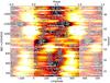 |
Fig. 5 Phase folded data, with the calculated spot longitudes over-plotted. The plot is extended a half phase in each direction to become more readable (shaded areas). |
3. Results
3.1. Spot configurations and stellar spot seasons
Since we are interested in localizing the spots on the stellar surface, we choose a five-spot model with variable positions and radii in the following. In Fig. 5 we show the results of our spot analysis for Kepler-210 by plotting the calculated − from the model − positions of the modeled spots vs. time (on the y-axis). The color-coded plot represents the phase-folded light curve, and the calculated spot longitudes are over-plotted at the appropriate spot longitudes. The size of each dot corresponds to the calculated size of the spot. The star spot sizes and longitudes show some interesting features in the behavior of the spots on Kepler-210. In the following we refer to time as the number of days elapsed since the date BJD = 2 454 833.0.
At the beginning of the Kepler observations the activity on Kepler-210 is concentrated into two regions centered between 0°−20° longitude and 180°−200° longitude. As a result one hemisphere is very active, i.e., the one between 0°−180°, while the other half of the star remains almost spotless.
By day ~350, the region at 180° appears to split up in two parts, one apparently moving towards smaller longitudes and the other towards larger longitudes. By day ~630, the region moving towards smaller longitudes disappears and the region remains spotless for about 200 days. At the same time activity appears at longitude 200°−300°, i.e., a region that was found inactive before. Also, the activity region at 0°−20° starts drifting towards larger longitudes. By day ~800, the activity in the longitude range 200°−300° disappears again and that range remains more or less spotless for the rest of the Kepler-210 observations. Between 800 days and 1000 days, three activity concentrations are visible, two at about 200° and 300° longitude moving towards smaller longitudes and the already mentioned region at 0°−20°, which is now moving towards larger longitudes. Between days 1000 and 1250, the activity appears to be concentrated more and less homogeneously between longitudes 50°−250°. By around day 1200, the activity near longitude 120° starts thinning out and the recognized two activity complexes are drifting towards smaller longitudes. Based on this phenomenology, we divide the data of Kepler-210 into six seasons S1 .... S6: S1: 130 days−350 days, S2: 350 days−600 days, S3: 600 days−800 days, S4: 800 days−1000 days, S5: 1000 days−1250 days and S6: 1250 days−1600 days.
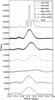 |
Fig. 6 L-S periodograms of each so-called stellar season. The solid line represents the total L-S periodogram of the light curve. The transition from small periods to longer and then gradually to small again resembles the butterfly diagram of the Sun (see Sects. 3.2 and 4.2). |
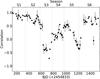 |
Fig. 7 Cross-correlation between the different phases with period P = 12.28 days. The outlying points in times ~750 days and ~1450 days originate to anomalies in the light curve due to the transition from one Kepler observation quarter to the next. |
3.2. Power spectrum analysis
The introduction of the so-called seasons in Sect. 3.1 was performed purely phenomenologically. We now calculate the L-S periodogram for each season (shown in Fig. 6) and note that the value of the maximum power periods varies from season to season, with exception of seasons S1 and S2. The L-S of season S3 has the smallest power, owing to the existence of multiple periodicities and the maximum power of this season appears to be at periods slightly larger than 12.6 days. Starting from season S3 and up to S6, there is an obvious diminution of the prominent period value from ~12.6 days to ~12.3 days. In general, the period range which we calculate for the different seasons explains the structure of the L-S diagram of the total light curve (continuous line), with exception of the peak at ~12.1 days, the origins of which we are not able to clarify.
3.3. Cross-correlation between the different light curve portions
Another method adequate to quantify any differences between the observed seasons is to compare the evolution of the light curve modulations in time. To that end, we separate the light curve in parts (phases) equal to the leading period of the L-S periodogram (i.e., 12.28 days) following the expression ![Mathematical equation: \begin{equation} \Phi_{i}\,=\,[t_{0}+P \cdot {i}\,,\,t_{0}+P\cdot ({i}+1)]\quad \mathrm{with}\quad {i}=0,1,2...N, \end{equation}](/articles/aa/full_html/2016/10/aa28491-16/aa28491-16-eq35.png) (2)where P, T0, and N denote the period, the time of the first observation, and the total number of phases respectively. In Fig. 7, we show the cross-correlation between the different phases Φi of the light curve and the phase Φ0 (reference phase). The error bars are inversely proportional to the common number of points per phase pair, i.e, zero error denotes equal number of points between the reference and the examined phase. In the same fashion as with the L-S periodogram, the seasons are also easily distinguishable in Fig. 7, marked by rapid changes in the cross-correlation between the phases.
(2)where P, T0, and N denote the period, the time of the first observation, and the total number of phases respectively. In Fig. 7, we show the cross-correlation between the different phases Φi of the light curve and the phase Φ0 (reference phase). The error bars are inversely proportional to the common number of points per phase pair, i.e, zero error denotes equal number of points between the reference and the examined phase. In the same fashion as with the L-S periodogram, the seasons are also easily distinguishable in Fig. 7, marked by rapid changes in the cross-correlation between the phases.
4. Physical interpretation
So far we have shown that the rotational periods of the active regions of Kepler-210 appear to vary in time. But what is the physical interpretation of the results of Sect. 3?
4.1. Active longitudes
There is a clear preference for some longitudes where spots prefer to appear, while other surface areas remain more or less spotless. Using our algorithm, we find that there is an area between 150° and 200° in longitude, which is covered by spots in every observed rotation of the star. On the other hand, about 100 degrees in longitude are covered by spots during only 20% of the total observation time.
4.2. Differential rotation
As discussed in Sect. 3, the leading period of the activity modulations of each season is different (see Fig. 6). Thus, in agreement with the claims of Reinhold et al. (2013), we interpret those changes as evidence for differential rotation, now assuming that the observed difference in period can be attributed to a difference in latitude. We specifically assume a solar-like differential rotation pattern with shorter rotation periods occurring near the equator. Furthermore, we can estimate the magnitude of the differential rotation as a function of the assumed spot latitude, assuming the same analytical form of the differential rotation law as applicable for the Sun: 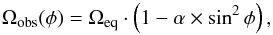 (3)with φ, Ωobs, and Ωeq denoting the latitude and the rotation rates at given latitudes and the equator, respectively. Our argument is also supported by the visible drifts of active regions in Fig. 5; the spot groups with larger periods than the phase-folding period (P = 12.28, see Fig. 6), appear with a small delay from one phase to the next, while the spot groups with shorter periods appear earlier. A nice example of these motions can be found in season S4, between 800 and 1000 days.
A characteristic of the Fig. 6 worth mentioning is the so-called jump of the spots from small latitudes (season S2) to larger latitudes (season S3), which is then followed by a smooth migration of the spots back to smaller latitudes. This behavior resembles the behavior of sunspots as they appear in the famous butterfly diagram for the Sun. During an 11-year magnetic cycle, the latitudes of the appearing sunspots first increase rapidly and then, gradually, move closer to the equator.
Given the fact that the peak to peak amplitude of the modulations is not reduced dramatically during season S3, we assume that the maximum latitude φmax of the spots ought to remain not too far away from the stellar equator, so that the reduction of the spotted areas (due to their projection) remains insignificant. To test this hypothesis we calculate the strength of the differential rotation α as a function of the stellar latitude φ using the equation
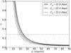 |
Fig. 8 Estimation of the differential rotation α of the star, assuming spots with rotational period Psp ≃ 12.6 days for latitudes between 0° and 90°. The dashed line indicates the value of the differential rotation of the Sun. |
 (4)where Pobs(φ) is the rotational period at a given stellar latitude φ and Peq denotes the equatorial rotational period. In Fig. 8, we plot our estimates for the differential rotation strength α, assuming different stellar latitudes φ for spots with rotational period 12.6 days (i.e., the spots which are assumed to be responsible for the peak close to ~12.6 days in the L-S of season S3), given three different values for the equatorial rotation period of the star. The dashed line in the same diagram indicates the value of the solar differential rotation, i.e., ~0.28 (Howard & Harvey 1970; Snodgrass & Ulrich 1990).
At this stage we cannot provide a direct connection between the observed rotational period of the spots and their latitudes. However, we can use our estimate for the strength of the differential rotation in Fig. 8 to put some constraints on the possible latitudes of the spots with rotational period Psp ≃ 12.6 days.
In Fig. 8, we see that the strength of the required differential rotation reaches values higher than that of the Sun, assuming that the latitudes of the spots with rotational period Psp ≃ 12.6 days have values lower than ~25°. As a result, we do not favor this assumption since it might not be easily explained by theory (e.g., Küker & Rüdiger 2008).
Furthermore, based on the assumption upon which we observe the star equator, the hypothesis that the spots of season S3 occupy latitudes larger than ~40° would require dramatic variations in the average spot sizes from one season to the next to maintain the relatively stable amplitude of ~2%, which we observe in the light curve of Kepler-210. We note that while the transits of Kepler-210 b are affected by spot-crossing events, the estimated size of those spots is not sufficient to produce the observed modulations.
Consequently, we suggest that the spots of season S3 with rotational period Psp ≃ 12.6 days ought to have latitudes in the range of between 25° ≲ φmax ≲ 40°. Incidentally, this is also the latitude range where we observe the sunspots with the highest latitudes, i.e., during the solar maximum. Following the hypothesis that the latitudes of the spots with rotational period Psp ≃ 12.6 days lay in the range 25° ≲ φmax ≲ 40°, the differential rotation of the star is similar and slightly smaller in comparison to the differential rotation of the Sun.
During seasons S3 and S4 another abnormal event takes place: It is the only time during the Kepler-210 observations when the area between ~200° and ~360° is covered by spots. At the same time, the rest of the usually spotted stellar surface becomes free of spots. Although the connection of this event to a physical process might not be trivial, it is an evidence that a dramatic change happened to the star during that season (see, Fig. 5).
4.3. Spot formation and spot life times
The observed flux variations of Kepler-210 are similar from one rotation to the next (see Figs 7). The latter fact suggests that the life time τsp of the active regions is much longer than the stellar rotation period P⋆.
In Fig. 1, we observe parts of the light curve where the peak-to-peak amplitude of the modulations is larger. Owing to the lack of a plateaued part in the light curve, we conclude that there is no time during the Kepler observations of Kepler-210 with a complete absence of spots on the visible hemisphere of the star. As a result, we assume that the short-term variations of the total spot coverage are the result of simultaneous occupations of stellar longitudes closer than the half visible hemisphere from different spot groups.
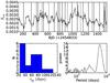 |
Fig. 9 Top: evolution of the size of the total spotted area, calculated as the summed area of the spots, which define the model for each light curve chunk. The vertical lines indicate the local minima of the curve. Bottom-left: distribution of the spot life times (see text for details). Bottom-right: L-S periodogram for the evolution of the spotted area size. |
There are two possibilities for such an association to occur; either a spot appears in an area with a neighboring longitude to a preexisting spot, or two spots with different stellar latitudes “meet” due to their differential rotation. From a visual examination of Fig. 5, we observe that both effects are taking place, with the former effect being more dominant. Therefore we suggest that it is possible to estimate the life time of the spots by measuring the duration of the simultaneous appearance of spot groups in the same stellar hemisphere.
Using the estimated spot radii we can calculate the total covered area (Srot) for each of the light curve chunks (see, Sect. 2.2.1 for details). The top panel of Fig. 9 shows the evolution of the total covered area as a function of time. As the duration of each fluctuation, we consider the range between two local minima of the covered area curve, which are marked with vertical lines in Fig. 9.
In the lower left panel of Fig. 9, we show the suggested spot lifetime distribution, which ranges between ~25 days and ~130 days. There are two maxima, one close to ~25 days and an other around ~90 days. After visual examination of Fig. 5, we can confirm that the duration of the dark features (spotted areas) varies between ~60 days and ~90 days. The peak close to ~25 days (see, Fig. 9) is probably a bias caused by the detection of consecutive local extrema in the curve of the total covered area.
The L-S periodogram of the spotted area, displayed in the lower right panel of Fig. 9, shows several low significance peaks for periods in the range between ~60 days and ~90 days. The most significant peak is found for a period around ~600 days. The long term variation responsible for this peak is visible in the upper panel of Fig. 9, where the total spotted area appears to become larger close to the end of season S2, then drops for seasons S3 and S4, and rises again in season S5.
5. Conclusions
Using the phenomenology of the Kepler-210 light curve in combination with the results of a five-spot model, we study the behavior of the spotted areas on the star (i.e., their relative periods and the longitudes at which they appear) and their changes in time (see Fig. 5). Based on the spot phenomenology we identify six different “spot seasons” and demonstrate that there are differences in the dominant periods of the L-S periodograms corresponding to each season (see Fig. 6). Additionally we show that the seasons also manifest themselves as differences in the correlation between the corresponding parts of the light curve (see Fig. 7).
According to Fig. 6, the relative period of spots in the subsequent seasons appears to change in the same fashion as the relative rotational period of sunspots during the solar cycle, i.e., the relative starspot period appears to change from lower to higher values between seasons S2 and S3,while it diminishes gradually from season S4 until the end of the Kepler observations. A common characteristic between all seasons, with the exception of seasons S3 and S4, is the persistent appearance of the spots in a specific longitude range of the star.
Assuming solar-like differential rotation we show that the value of the strength of the differential rotation α ought to be similar or lower to that of the Sun under the hypothesis that the spots with the higher periods have latitudes in the range of between 25° ≲ φmax ≲ 40° (see Fig. 8). Furthermore, we estimate the spot life times using the radii of the spots that were computed with our model fit. As a result, we conclude that the spot life times of Kepler-210 vary between ~60 days and ~90 days (see Figs. 5 and 9).
The behavior of the active regions on the photosphere of Kepler-210 (i.e., the shift from small asterographic latitudes to higher and vice versa) is comparable to the migration of sunspots during an 11-year solar magnetic cycle (see Fig. 6). We estimate that the duration of this phenomenon on Kepler-210 is similar, or somewhat longer, than the total Kepler observation time (i.e., ~4 years), however, additional long-term observations are clearly needed to check whether this behavior of Kepler-210 as observed by Kepler is actually periodic and indeed the result of a magnetic cycle.
Acknowledgments
P.I. acknowledges funding through the DFG grant RTG 1351/2 Extrasolar planets and their host stars.
References
- Alonso, R., Auvergne, M., Baglin, A., et al. 2008, A&A, 482, L21 [NASA ADS] [CrossRef] [EDP Sciences] [Google Scholar]
- Baglin, A., Auvergne, M., Barge, P., et al. 2006, in ESA SP 1306, eds. M. Fridlund, A. Baglin, J. Lochard, & L. Conroy, 33 [Google Scholar]
- Bonomo, A. S., & Lanza, A. F. 2012, A&A, 547, A37 [NASA ADS] [CrossRef] [EDP Sciences] [Google Scholar]
- Borucki, W. J., Koch, D., Basri, G., et al. 2010, Science, 327, 977 [NASA ADS] [CrossRef] [PubMed] [Google Scholar]
- Chabrier, G., & Küker, M. 2006, A&A, 446, 1027 [NASA ADS] [CrossRef] [EDP Sciences] [Google Scholar]
- Fabrycky, D. C., Lissauer, J. J., Ragozzine, D., et al. 2014, ApJ, 790, 146 [NASA ADS] [CrossRef] [Google Scholar]
- Fang, J., & Margot, J.-L. 2012, ApJ, 761, 92 [NASA ADS] [CrossRef] [Google Scholar]
- Figueira, P., Marmier, M., Boué, G., et al. 2012, A&A, 541, A139 [NASA ADS] [CrossRef] [EDP Sciences] [Google Scholar]
- Frasca, A., Fröhlich, H.-E., Bonanno, A., et al. 2011, A&A, 532, A81 [NASA ADS] [CrossRef] [EDP Sciences] [Google Scholar]
- Fröhlich, H.-E., Küker, M., Hatzes, A. P., & Strassmeier, K. G. 2009, A&A, 506, 263 [NASA ADS] [CrossRef] [EDP Sciences] [Google Scholar]
- Howard, R., & Harvey, J. 1970, Sol. Phys., 12, 23 [NASA ADS] [CrossRef] [Google Scholar]
- Huber, K. F., Czesla, S., Wolter, U., & Schmitt, J. H. M. M. 2009, A&A, 508, 901 [NASA ADS] [CrossRef] [EDP Sciences] [Google Scholar]
- Ioannidis, P., Schmitt, J. H. M. M., Avdellidou, C., von Essen, C., & Agol, E. 2014, A&A, 564, A33 [NASA ADS] [CrossRef] [EDP Sciences] [Google Scholar]
- Johansen, A., Davies, M. B., Church, R. P., & Holmelin, V. 2012, ApJ, 758, 39 [NASA ADS] [CrossRef] [Google Scholar]
- Kinemuchi, K., Barclay, T., Fanelli, M., et al. 2012, PASP, 124, 963 [NASA ADS] [CrossRef] [Google Scholar]
- Küker, M., & Rüdiger, G. 2008, J. Phys. Conf. Ser., 118, 012029 [NASA ADS] [CrossRef] [Google Scholar]
- McQuillan, A., Aigrain, S., & Roberts, S. 2012, A&A, 539, A137 [NASA ADS] [CrossRef] [EDP Sciences] [Google Scholar]
- McQuillan, A., Mazeh, T., & Aigrain, S. 2014, ApJS, 211, 24 [NASA ADS] [CrossRef] [MathSciNet] [Google Scholar]
- Morton, T. D., & Winn, J. N. 2014, ApJ, 796, 47 [NASA ADS] [CrossRef] [Google Scholar]
- Petigura, E. A., & Marcy, G. W. 2012, PASP, 124, 1073 [NASA ADS] [CrossRef] [Google Scholar]
- Reinhold, T., & Reiners, A. 2013, A&A, 557, A11 [NASA ADS] [CrossRef] [EDP Sciences] [Google Scholar]
- Reinhold, T., Reiners, A., & Basri, G. 2013, A&A, 560, A4 [NASA ADS] [CrossRef] [EDP Sciences] [Google Scholar]
- Snodgrass, H. B., & Ulrich, R. K. 1990, ApJ, 351, 309 [Google Scholar]
- Stumpe, M. C., Smith, J. C., Van Cleve, J. E., et al. 2012, PASP, 124, 985 [NASA ADS] [CrossRef] [Google Scholar]
- Tremaine, S., & Dong, S. 2012, AJ, 143, 94 [NASA ADS] [CrossRef] [Google Scholar]
- Zechmeister, M., & Kürster, M. 2009, A&A, 496, 577 [NASA ADS] [CrossRef] [EDP Sciences] [Google Scholar]
All Figures
|
Fig. 1 Complete light curve of the Kepler-210 (~1400 days), normalized and with the planetary transits excluded (see text for details). |
| In the text | |
|
Fig. 2 Amplitude of the simulated light curves residuals after the subtraction of the fitted equatorial spot model. The red lines show the mean variation of the modulations from one rotation to the next (solid red line) and its uncertainty (dashed red lines). The blue solid line represents the level of the Gaussian noise of the Kepler-210 light curve. |
| In the text | |
|
Fig. 3 χ2 goodness of the fit for models with different number of equally separated spots (upper panel) and free spots (lower panel). It is clear that the normalized χ2 is approaching close to unity for models with at least 10 free parameters (see text for details). |
| In the text | |
|
Fig. 4 Top: visual representation of the 10 fixed spot model. Each of the thin colored lines represents the flux reduction caused from each of the spots during a full rotation. The combined flux reduction is given from the aggregation of the five spots models (thick red line). Bottom: as for top panel, but for the five-spot model. |
| In the text | |
|
Fig. 5 Phase folded data, with the calculated spot longitudes over-plotted. The plot is extended a half phase in each direction to become more readable (shaded areas). |
| In the text | |
|
Fig. 6 L-S periodograms of each so-called stellar season. The solid line represents the total L-S periodogram of the light curve. The transition from small periods to longer and then gradually to small again resembles the butterfly diagram of the Sun (see Sects. 3.2 and 4.2). |
| In the text | |
|
Fig. 7 Cross-correlation between the different phases with period P = 12.28 days. The outlying points in times ~750 days and ~1450 days originate to anomalies in the light curve due to the transition from one Kepler observation quarter to the next. |
| In the text | |
|
Fig. 8 Estimation of the differential rotation α of the star, assuming spots with rotational period Psp ≃ 12.6 days for latitudes between 0° and 90°. The dashed line indicates the value of the differential rotation of the Sun. |
| In the text | |
|
Fig. 9 Top: evolution of the size of the total spotted area, calculated as the summed area of the spots, which define the model for each light curve chunk. The vertical lines indicate the local minima of the curve. Bottom-left: distribution of the spot life times (see text for details). Bottom-right: L-S periodogram for the evolution of the spotted area size. |
| In the text | |
Current usage metrics show cumulative count of Article Views (full-text article views including HTML views, PDF and ePub downloads, according to the available data) and Abstracts Views on Vision4Press platform.
Data correspond to usage on the plateform after 2015. The current usage metrics is available 48-96 hours after online publication and is updated daily on week days.
Initial download of the metrics may take a while.