| Issue |
A&A
Volume 593, September 2016
|
|
|---|---|---|
| Article Number | L17 | |
| Number of page(s) | 3 | |
| Section | Letters | |
| DOI | https://doi.org/10.1051/0004-6361/201629257 | |
| Published online | 23 September 2016 | |
A simple explanation of the linear rms–mean flux relation in accreting objects
Department of Statistics, University of the Western Cape, Private Bag X17, Bellville, 7535 Cape, South Africa
e-mail: ckoen@uwc.ac.za
Received: 6 July 2016
Accepted: 4 September 2016
Aims. We provide an alternative to existing theories for the origin of linear rms–mean flux relations observed in a variety of accreting systems, from AGN to white dwarfs.
Methods. Standard statistical theory and simulations are used to explore the possibility that the relations are due to simple scaling effects.
Results. The proposed theory can reproduce the unit slope of the rms–mean flux relation observed in the most extensive study published to date. The close similarity of the fractional variability in different objects deserves further study.
Key words: accretion, accretion disks / methods: statistical
© ESO, 2016
1. Introduction
A number of papers have drawn attention to linear relations between the mean flux level and the root mean square (rms) of flux variations, as observed in a variety of accreting astronomical objects. Some of the relevant papers are Uttley & McHardy (2001; active galactic nuclei and a millisecond pulsar), Gleissner et al. (2004; a black hole), Van de Sande et al. (2015; white dwarfs), and Zamanov et al. (2016; white dwarfs and symbiotic stars). Further references are available in these sources.
Uttley et al. (2005) proposed an explanatory model for these linear rms–mean relations. Key ingredients are non-linearity of the light curves, and lognormal flux distributions. An alternative interpretation of the relations is presented below in terms of simple statistical identities. No specific distributional assumptions or forms of the time series are required.
2. Statistical model
Understanding the model is facilitated by thinking of the light curve of the accreting system as the manifestation of a stochastic process, consisting of a succession of values of a random variable X. The random process has mean
 where E is the expectation (ensemble mean) operator, while the standard deviation (rms) of its variations is given by
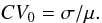
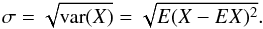 Another useful statistic is the coefficient of variation, defined as
 First we consider the simple situation where the process switches to a new mean level. If the flux increases by a factor β, so that X → βX, then the following simple standard statistical relations hold:
![\begin{eqnarray} &&{E}(\beta X) = \beta \mu \nonumber\\ &&{\rm var}(X) = {E}\left [(\beta X)-{E}(\beta X)\right]^2\nonumber\\ && \qquad \quad = \beta^2 \sigma^2\nonumber\\ &&CV = \sqrt{\beta^2 \sigma^2}/(\beta \mu) \equiv CV_0. \end{eqnarray}](/articles/aa/full_html/2016/09/aa29257-16/aa29257-16-eq8.png) (1)Obviously then, if X switches between any number of well-defined mean levels, the coefficient of variation (or fractional variability) remains constant at CV0.
(1)Obviously then, if X switches between any number of well-defined mean levels, the coefficient of variation (or fractional variability) remains constant at CV0.
For an illustrative example of what happens if the mean level is continuously variable, the reader is referred to the simulated dataset plotted in Fig. 1. Here, 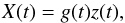 (2)where g(t) is a smooth trend (an integrated random walk in this example), and z(t) is Gaussian with mean 20 and standard deviation 1 (arbitrary illustrative values).
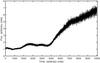 |
Fig. 1 A simulated dataset X(t), consisting of Gaussian white noise z(t) multiplied by a smooth trend function g(t). |
The series in Fig. 1 is then subdivided into bins, and the mean and standard deviations of the points X(t) in each bin calculated. The results are plotted in Fig. 2 for a few different bin widths (or timescales). For comparison, the lines
 are also plotted; they correspond to the constant coefficient of variation CV = 0.05. Clearly the expected rms–mean relation is obtained, regardless of the choice of bin width.
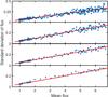 |
Fig. 2 Relation between the MSE and the mean for the light curve in Fig. 1. The simulated data were subdivided into bins, and the means and standard deviations of the values in each bin calculated. Bin widths, from top to bottom, are 25, 50, 100, and 200 points. The straight lines correspond to constant coefficients of variation of 0.05. |
Figure 3 shows a second simulated dataset, again with an integrated random walk as the trend function. The model for the random process is more realistic: instead of white noise, z(t) in (2) is taken to be an autoregressive (AR) series 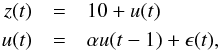 where α is a constant (equal to 0.9 in Fig. 3), and ϵ(t) is white noise with standard deviation σϵ = 0.1. The variance of z(t) in this case is
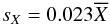
 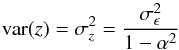 (3)(e.g. Chatfield 2003). It follows that σz = 0.23 and CV = 0.023.
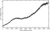 |
Fig. 3 A simulated dataset X(t), consisting of a first-order autoregressive time series z(t) multiplied by a smooth trend function g(t). |
The equivalent of Fig. 2 is plotted in Fig. 4, which is based on the data in Fig. 3. Comparison with Fig. 2 shows that although linear rms–mean flux relations persist, the exact form is now dependent on the bin size. In particular, for large bin sizes the expected forms
 are recovered, whereas for small bins the slopes systematically decrease with bin size.
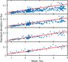 |
Fig. 4 Relation between the MSE and the mean for the light curve in Fig. 3. The simulated data were subdivided into bins, and the means and standard deviations of the values in each bin calculated. Bin widths, from top to bottom, are 25, 50, 100, and 200 points. The straight lines correspond to constant coefficients of variation of 0.023. |
The explanation of the dependence on bin size (or timescale) lies in the form of the variability of the adopted AR time series – see Fig. 5 for three realisations. It is clear that as α increases, sustained deviations from the mean also increase; which explains why σz increases with α in (3). Since the “coherence time” of these deviations increases with α, longer sections of the time series are needed to plumb the full extent of the deviations from the mean, i.e. the variance of the series. Conversely, if short stretches of the time series (i.e. small bin sizes) are used to estimate  , the variance will be underestimated.
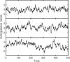 |
Fig. 5 Three AR time series with respective coefficients α = 0.85 (top), α = 0.9 (middle), and α = 0.95 (bottom). |
In the frequency domain the power spectral density (PSD) is of interest: at frequency ω it is defined as ![\begin{eqnarray} f_X(\omega)&=&c \sum_{k=-\infty}^\infty \gamma_X(k)\, {\rm e}^{-{\rm i}\omega k} \nonumber\\ \gamma_X(k)&=&{E}\left [X(t)-{E}X(t)\right] \left [X(t+k)- {E}X(t+k) \right],\nonumber \end{eqnarray}](/articles/aa/full_html/2016/09/aa29257-16/aa29257-16-eq30.png) where c is a normalising constant and γX is the autocovariance function of the series X. If X is scaled by β, the PSD is scaled by β2 at all frequencies – in other words, the scaling holds at all timescales (as is evident especially from Fig. 2). In this regard, see also Uttley & McHardy (2001), who note that the amplitudes of the PSD of the accreting stars change with time, while their shapes remain unchanged.
where c is a normalising constant and γX is the autocovariance function of the series X. If X is scaled by β, the PSD is scaled by β2 at all frequencies – in other words, the scaling holds at all timescales (as is evident especially from Fig. 2). In this regard, see also Uttley & McHardy (2001), who note that the amplitudes of the PSD of the accreting stars change with time, while their shapes remain unchanged.
3. Discussion
An overview, and expansion, of the material in the previous section follows:
-
(i)
Light curves are interpreted as being due to stochasticprocesses. If the flux switches from constant mean level μ1 to level μ2, then the ratio of first to second standard deviations will be μ1/μ2, i.e. the coefficient of variation will remain unchanged.
-
(ii)
If the function g(t) in (2) is deterministic, for example a low-order polynomial, then
![\begin{eqnarray} {E}[X(t)] &=& g(t) {E}[z(t)] \nonumber\\ {\rm var}[X(t)] &=& g^2(t) {\rm var}[z(t)] \nonumber\\ CV(X) &=& \sqrt{{\rm var}[X(t)]}/{E}[X(t)]\nonumber\\ &=& \sqrt{{\rm var}[z(t)]}/{E}[z(t)]\nonumber\\ &\equiv& CV(z), \nonumber \end{eqnarray}](/articles/aa/full_html/2016/09/aa29257-16/aa29257-16-eq37.png) i.e. the coefficients of variation of the processes X(t) and z(t) are identical. This means that
i.e. the coefficients of variation of the processes X(t) and z(t) are identical. This means that ![$${\rm rms}[X(t)]=CV {\rm mean}[X(t)]$$](/articles/aa/full_html/2016/09/aa29257-16/aa29257-16-eq38.png) at each timepoint t, where CV is constant.
at each timepoint t, where CV is constant. -
(iii)
If the flux level is modulated slowly with time by a random trend, as in Figs. 1 and 3, the situation is unchanged, provided the light curve sections which are compared are short compared to the timescale of the trend. For a light curve section centred on time t = t0,
![\begin{eqnarray} {E}[X(t)] & \approx & g(t_0) {E}[z(t)] \nonumber\\ {\rm var}[X(t)] & \approx & g^2(t_0) {\rm var}[z(t)] \nonumber\\ CV(X) & \approx & CV(z). \nonumber \end{eqnarray}](/articles/aa/full_html/2016/09/aa29257-16/aa29257-16-eq42.png)
-
(iv)
If measurement errors are negligible, then clearly a linear rms–mean relation should have zero intercept. This is exactly equivalent to a constant coefficient of variation. In the presence of measurement errors such that Y = X + e,
 and the intercept will be non-zero. Provided measurement errors and the process X are uncorrelated, and
  ,
, ![\begin{eqnarray} {\rm rms}(Y) & \approx & \left [1+\frac{1}{2} \sigma_e^2/ {\rm var}X \right]{\rm rms}(X)\nonumber\\[3mm] &=& CV(X) \left [1+\frac{1}{2} \sigma_e^2/ {\rm var}X \right]{E}(Y)\nonumber. \end{eqnarray}](/articles/aa/full_html/2016/09/aa29257-16/aa29257-16-eq46.png)
-
(v)
If the stochastic process is strongly autocorrelated, its intrinsic rms will be underestimated over short sections of the light curve. However, provided long enough stretches of the light curve are used, the expected rms–mean relations are recovered.
4. Comparison to Zamanov et al. (2016)
Zamanov et al. (2016) obtained several photometric runs on each of nine systems, namely seven cataclysmic variables and two symbiotic stars. In total, 204 light curves were collected. Plotted in a log (rms) – log (mean flux) diagram, all but seven points (corresponding to the same star) lie along a well-defined straight line with a slope of 0.994 (standard error 0.042). This is exactly what is expected for constant coefficients of variation: 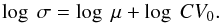 (4)Although Eq. (4) could have been anticipated on the basis of (1) for a single object, it is remarkable that Zamanov et al. (2016) obtained such closely similar coefficients of variation (0.086 ± 0.011) for all their objects. This may have something to do with the fact that the accreting stars in all the binary systems they observed were white dwarfs.
5. Conclusions
It was demonstrated in Sect. 2 that linear rms–mean flux relations are obtained if a stochastic sequence is subject to simple scaling as in Eq. (2). In that equation, z(t) is an arbitrary stochastic process, and g(t) is a slowly varying modulating function. The physics underlying z(t) and g(t) does not have to be coupled: a constant coefficient of variation of their product X(t) will result provided g(t) is smooth. A prime candidate for the scaling function g(t) is small amplitude variability in the supply of accreting material onto the surface of the accreting object (e.g. Bruch 1992). The only requirement is that the variability timescale be long compared to that of the stochastic process z(t) giving rise to the observed light curves.
Acknowledgments
This work was partially supported by a grant from the South African National Research Foundation. A lunchtime conversation with Prof. Brian Warner stimulated this Letter.
References
- Bruch, A. 1992, A&A, 266, 237 [NASA ADS] [Google Scholar]
- Chatfield, C. 2003, The Analysis of Time Series: an Introduction 6th edn. (London: Chapman & Hall/CRC Press) [Google Scholar]
- Gleissner, T., Wilms, J., Pottschmidt, K., et al. 2004, A&A, 414, 1091 [NASA ADS] [CrossRef] [EDP Sciences] [Google Scholar]
- Uttley, P., & McHardy, I. M. 2001, MNRAS, 323, L26 [NASA ADS] [CrossRef] [Google Scholar]
- Uttley, P., & McHardy, I. M., Vaughan, S. 2005, MNRAS, 359, 345 [NASA ADS] [CrossRef] [Google Scholar]
- Van de Sande, M., Scaringi, S., & Knigge, C. 2015, MNRAS, 448, 2430 [NASA ADS] [CrossRef] [Google Scholar]
- Zamanov, R. K., Boeva, S., Latev, G., et al. 2016, MNRAS, 457, L10 [NASA ADS] [CrossRef] [Google Scholar]
All Figures
|
Fig. 1 A simulated dataset X(t), consisting of Gaussian white noise z(t) multiplied by a smooth trend function g(t). |
| In the text | |
|
Fig. 2 Relation between the MSE and the mean for the light curve in Fig. 1. The simulated data were subdivided into bins, and the means and standard deviations of the values in each bin calculated. Bin widths, from top to bottom, are 25, 50, 100, and 200 points. The straight lines correspond to constant coefficients of variation of 0.05. |
| In the text | |
|
Fig. 3 A simulated dataset X(t), consisting of a first-order autoregressive time series z(t) multiplied by a smooth trend function g(t). |
| In the text | |
|
Fig. 4 Relation between the MSE and the mean for the light curve in Fig. 3. The simulated data were subdivided into bins, and the means and standard deviations of the values in each bin calculated. Bin widths, from top to bottom, are 25, 50, 100, and 200 points. The straight lines correspond to constant coefficients of variation of 0.023. |
| In the text | |
|
Fig. 5 Three AR time series with respective coefficients α = 0.85 (top), α = 0.9 (middle), and α = 0.95 (bottom). |
| In the text | |
Current usage metrics show cumulative count of Article Views (full-text article views including HTML views, PDF and ePub downloads, according to the available data) and Abstracts Views on Vision4Press platform.
Data correspond to usage on the plateform after 2015. The current usage metrics is available 48-96 hours after online publication and is updated daily on week days.
Initial download of the metrics may take a while.