| Issue |
A&A
Volume 593, September 2016
|
|
|---|---|---|
| Article Number | A91 | |
| Number of page(s) | 12 | |
| Section | Extragalactic astronomy | |
| DOI | https://doi.org/10.1051/0004-6361/201628447 | |
| Published online | 29 September 2016 | |
Long-term multi-wavelength variability and correlation study of Markarian 421 from 2007 to 2009⋆
1 ETH Zurich, 8093 Zurich, Switzerland
2 Università di Udine, and INFN Trieste, 33100 Udine, Italy
3 INAF National Institute for Astrophysics, 00136 Rome, Italy
4 Università di Siena, and INFN Pisa, 53100 Siena, Italy
5 Croatian MAGIC Consortium, Rudjer Boskovic Institute, University of Rijeka, University of Split and University of Zagreb, Croatia
6 Saha Institute of Nuclear Physics, 1/AF Bidhannagar, Salt Lake, Sector-1, 700064 Kolkata, India
7 Max-Planck-Institut für Physik, 80805 München, Germany
8 Universidad Complutense, 28040 Madrid, Spain
9 Inst. de Astrofísica de Canarias, 38200 La Laguna; Universidad de La Laguna, Dpto. Astrofísica, 38206 La Laguna, Tenerife, Spain
10 University of Łódź, 90236 Lodz, Poland
11 Deutsches Elektronen-Synchrotron (DESY), 15738 Zeuthen, Germany
12 Institut de Fisica d’Altes Energies (IFAE), The Barcelona Institute of Science and Technology, Campus UAB, 08193 Bellaterra (Barcelona), Spain
13 Universität Würzburg, 97074 Würzburg, Germany
14 Università di Padova and INFN, 35131 Padova, Italy
15 Institute for Space Sciences (CSIC/IEEC), 08193 Barcelona, Spain
16 Technische Universität Dortmund, 44221 Dortmund, Germany
17 Unitat de Física de les Radiacions, Departament de Física, and CERES-IEEC, Universitat Autònoma de Barcelona, 08193 Bellaterra, Spain
18 Universitat de Barcelona, ICC, IEEC-UB, 08028 Barcelona, Spain
19 Japanese MAGIC Consortium, ICRR, The University of Tokyo, Department of Physics and Hakubi Center, Kyoto University, Tokai University, The University of Tokushima, KEK, Japan
20 Finnish MAGIC Consortium, Tuorla Observatory, University of Turku and Astronomy Division, University of Oulu, 90014 Oulu, Finland
21 Inst. for Nucl. Research and Nucl. Energy, 1784 Sofia, Bulgaria
22 Università di Pisa, and INFN Pisa, 56126 Pisa, Italy
23 ICREA and Institute for Space Sciences (CSIC/IEEC), 08193 Barcelona, Spain
24 Centro Brasileiro de Pesquisas Físicas (CBPF/MCTI), R. Dr. Xavier Sigaud, 150 – Urca, 22290-180 Rio de Janeiro, Brazil
25 NASA Goddard Space Flight Center, Greenbelt, MD 20771; and Department of Physics and Department of Astronomy, University of Maryland, College Park, MD 20742, USA
26 Humboldt University of Berlin, Institut für Physik Newtonstr. 15, 12489 Berlin, Germany
27 École polytechnique fédérale de Lausanne (EPFL), Lausanne, Switzerland
28 Japanese MAGIC Consortium, Kyoto, Japan
29 Finnish Centre for Astronomy with ESO (FINCA), Turku, Finland
30 INAF-Trieste, 34143 Trieste, Italy
31 ISDC – Science Data Center for Astrophysics, 1290 Versoix, (Geneva), Switzerland
32 Astron. Inst., St.-Petersburg State Univ., 198504 St. Petersbourg, Russia
33 University of Crete, Heraklion, Greece
34 Graduate Institute of Astronomy, National Central University, 300 Zhongda Rd, 32001 Zhongli, Taoyuan, Taiwan
35 Pulkovo Observatory, 196140 St.-Petersburg, Russia
36 Agrupació Astronòmica de Sabadell, 08206 Sabadell, Barcelona, Spain
37 Aalto University Metsähovi Radio Observatory, Metsähovintie 114, 02540 Kylmälä, Finland
38 School of Cosmic Physics, Dublin Institute For Advanced Studies, Dublin 2, Ireland
39 Abastumani Observatory, Mt. Kanobili, 0301 Abastumani, Georgia
40 Engelhardt Astronomical Observatory, Kazan Federal University, Tatarstan, Russia
41 Aalto University Department of Radio Science and Engineering, PO BOX 13000, 00076 Aalto, Finland
42 Circolo Astrofili Talmassons, via Cadorna, 57, 33030 Talmassons, Italy
43 School of Physics, University College Dublin, Belfield, Dublin 4, Ireland
44 INAF–Osservatorio Astrofisico di Torino, 10025 Pino Torinese (TO), Italy
45 Department of Physics, University of Colorado, Denver, CO 80217-3364, USA
Received: 7 March 2016
Accepted: 23 May 2016
Aims. We study the multi-band variability and correlations of the TeV blazar Mrk 421 on year timescales, which can bring additional insight on the processes responsible for its broadband emission.
Methods. We observed Mrk 421 in the very high energy (VHE) γ-ray range with the Cherenkov telescope MAGIC-I from March 2007 to June 2009 for a total of 96 h of effective time after quality cuts. The VHE flux variability is quantified using several methods, including the Bayesian Block algorithm, which is applied to data from Cherenkov telescopes here for the first time. The 2.3 yr long MAGIC light curve is complemented with data from the Swift/BAT and RXTE/ASM satellites and the KVA, GASP-WEBT, OVRO, and Metsähovi telescopes from February 2007 to July 2009, allowing for an excellent characterisation of the multi-band variability and correlations over year timescales.
Results. Mrk 421 was found in different γ-ray emission states during the 2.3 yr long observation period: The flux above 400 GeV spans from the minimum nightly value of (1.3 ± 0.4)×10-11 cm-2 s-1 to the maximum flux, that is about 24 times higher, at (3.1 ± 0.1)×10-10 cm-2 s-1. Flares and different levels of variability in the γ-ray light curve could be identified with the Bayesian Block algorithm. The same behaviour of a quiet and active emission was found in the X-ray light curves measured by Swift/BAT and the RXTE/ASM, with a direct correlation in time. The behaviour of the optical light curve of GASP-WEBT and the radio light curves by OVRO and Metsähovi are different as they show no coincident features with the higher energetic light curves and a less variable emission. Overall, the fractional variability increases with energy. The comparable variability in the X-ray and VHE bands and their direct correlation during both high- and low-activity periods spanning many months show that the electron populations radiating the X-ray and γ-ray photons are either the same, as expected in the synchrotron-self-Compton mechanism, or at least strongly correlated, as expected in electromagnetic cascades.
Key words: astroparticle physics / BL Lacertae objects: individual: Markarian 421 / radiation mechanisms: non-thermal
The complete data set shown in Fig. 2 and the data points shown in Figs. 3 and 4 are only available at the CDS via anonymous ftp to cdsarc.u-strasbg.fr (130.79.128.5) or via http://cdsarc.u-strasbg.fr/viz-bin/qcat?J/A+A/593/A91
© ESO, 2016
1. Introduction
Markarian 421 (Mrk 421) is a high-frequency peaked BL Lac object (HBL) at a redshift of z = 0.030 (Piner et al. 1999). It was the first extragalactic TeV emitter to be detected (Punch et al. 1992).
Blazars are active galactic nuclei (AGN) where the jet is aligned to our line-of-sight. This means that it is possible to observe very high energy (VHE) γ-rays that are produced inside the jets and relativistically beamed in our direction. Additionally, AGN emit radiation over the whole electromagnetic spectrum, from radio wavelengths to VHE γ-rays.
Blazars feature a spectral energy distribution (SED) with a two-bump structure. The low energy component is due to the synchrotron radiation caused by electrons of the relativistic beam, while the high energy peaked bump is attributed to other interactions. This could be the Compton scattering of less energetic photons by the same electron population in leptonic scenarios or these photons could be produced inside hadronic interactions of, for example, protons in the jet. In HBL objects as Mrk 421, the Synchrotron bump covers the energy range from radio to X-ray wavelengths while the peak can be found between UV and X-ray wavelengths. The second bump extends from low-energy γ-rays to VHE γ-rays.
A characteristic feature of blazars, and of Mrk 421 in particular, is that they show states of high activity in which the emitted electromagnetic radiation can increase by more than one order of magnitude on timescales ranging from years down to minutes. During high states blazars often show significant spectral flux changes, and up to some extent, correlated flux variations in the low- and high-energy bumps. This blazar variability is an extraordinary opportunity to break degeneracies between the various emission models. Different models produce flux variations (at a given energy band) with particles of different energies, cooling times, and cross sections for different processes, and thus are in principle distinguishable. It is also important to note that the blazar emission zone is unresolved for all instruments (with perhaps the exception of radio Very Long Baseline Array (VLBA) interferometric observations), and hence variability is the only way of probing its structure. Therefore, while “snapshot” multi-wavelength (MWL) spectra provide us with clues on the emission mechanisms and physical parameters inside relativistic jets, detailed studies of time variability bring us additional information on the emission mechanisms and on the structure and the dynamics of the jet itself.
Mrk 421 has shown periods of large X-ray and γ-ray activity of various timescales, as reported previously in various publications (e.g. Gaidos et al. 1996; Cui 2004; Tluczykont et al. 2010). Mrk 421 has been the target of several past MWL campaigns, with the correlation between X-rays and TeV γ-rays as one of the key features under investigation. The details in the correlation between these two bands in Mrk 421 is crucial because it relates to the energy regions where most of the power is emitted (approximately the peaks of the two SED bumps), and hence the regions of the SED which can best distinguish between different theoretical scenarios.
A direct correlation between X-rays and TeV γ-rays has been reported multiple times during flaring activity (Macomb et al. 1995; Buckley et al. 1996; Fossati et al. 2004, 2008; Albert et al. 2007; Bartoli et al. 2011; Donnarumma et al. 2009; Abdo et al. 2011; Acciari et al. 2011; Cao & Wang 2013; Aleksić et al. 2015b). Recently, Aleksić et al. (2015a) and Baloković et al. (2016) also reported the existence of this correlation during low activity. Błażejowski et al. (2005) and Horan et al. (2009) were able to constrain the correlation to time differences below 1.5 days. These results are in agreement with the synchrotron-self-Compton (SSC) model, where the photons from both X-ray and γ-ray energies are produced by the same electron population. Other authors reported orphan flares in TeV γ-rays without an X-ray counterpart, which were observed in Mrk 421 during a MWL campaign in 2003 and 2004 (Błażejowski et al. 2005), unable to be explained by the SSC model. In Acciari et al. (2009) a correlation between TeV and X-rays is not found, and a possible hadronic origin of the emission is discussed. However, this correlation study relates to short observations (two half-day long observations) with very low variability. The X-ray emission was accurately characterized with continuous XMM observations, and flux variations at the level of 10% could be significantly resolved. Yet the TeV γ-ray measurements covered only a small fraction of the XMM observations, and had relatively large error bars. Therefore, the presented X-ray/TeV correlation results in Acciari et al. (2009) were not conclusive, and show very clearly the importance of having long, well sampled and sensitive TeV γ-ray observations to perform this kind of study.
Other energy bands are not evidently correlated with X-rays and TeV γ-rays. Macomb et al. (1995), Albert et al. (2007), Cao & Wang (2013) report a missing correlation of the optical and UV emission to the X-ray and TeV γ-ray emission. Confirming the trend of a strong correlation between X-rays and VHE, the work of Baloković et al. (2016) also reports a lack of correlation between optical/UV and X-rays, and moreover ascribes the observed broadband variability features during low activity to in situ electron acceleration in multiple compact regions. In Horan et al. (2009) a correlation with a time lag between the optical and the TeV γ-ray light curves is found, once with the optical features leading the TeV features and once vice versa, but the likelihood of having observed the optical leading and lagging the TeV features by chance is 20% and 60% respectively. In Aleksić et al. (2015a) an anti-correlation between the optical and UV light curves with the X-ray light curves is reported, but with the possibility that it might have been found by chance, proposing a dedicated correlation analysis over many years to properly characterize the temporal evolution of the optical and X-ray/TeV γ-ray bands.
Evidence of a correlation between radio and γ-ray activity was reported in Katarzyński et al. (2003), where the study of a single radio outburst with a X-ray and TeV γ-ray counterpart in February−March 2001 is presented. The author models a scenario in which the acceleration of electrons in the middle part of the jet describes well the temporal evolution of such a multispectral flare.
In the more recent work of Lico et al. (2014) a marginally significant correlation between radio and GeV γ-rays (without time lag) is reported. This study used observations spanning many months from 2011, when Mrk 421 did not show any flaring activity, hence suggesting a co-location of the radio and γ-ray emission of Mrk 421 during typical (low) activity.
A different result is derived from the outstanding radio activity observed in September 2012, where Mrk 421 showed a particularly symmetric flare profile, with the highest radio flux measured in three decades, as reported in Max-Moerbeck et al. (2014) and Hovatta et al. (2015). Both works assume that this giant radio flare is physically connected to a large γ-ray flaring activity measured by Fermi-LAT about one month before, and Max-Moerbeck et al. (2014) uses this time difference to locate the origin of the γ-ray emission upstream of the radio emission.
Because of the above-mentioned complexity and sometimes controversy in the multi-band flux variations and correlations observed during relatively short (weeks to months) campaigns, we need very long (multi-year) campaigns to put things into context. In this paper we report an extensive study of the multi-band flux variability of Mrk 421 during the 2.3 yr long period that spans from February 2007 to July 2009. We adopted the methodology reported in Aleksić et al. (2015a), which had been applied in a much shorter multi-instrument data set.
There are several publications that report studies with the VHE γ-ray emission of Mrk 421 during the above-mentioned 2.3 yr long period; yet they typically relate to smaller temporal intervals. For instance, Aleksić et al. (2012) reported MAGIC observations of a high active state performed from December 2007 to June 2008, and Abdo et al. (2011) and Aleksić et al. (2015a) reported results related to observations from a 4.5 month long time interval from January to June 2009. A very interesting study using Whipple 10 m observations performed from December 1995 to May 2009 was reported in Acciari et al. (2014), which allowed study of the duty cycle and evaluation of the VHE emission and its correlation with the X-ray emission. The study that we report in this paper relates to a time period that is (almost) contained in Acciari et al. (2014), but it provides a large number of improvements such as the larger sensitivity of MAGIC with respect to Whipple 10 m, which allows us to resolve the VHE flux with smaller uncertainties, and hence to study the variability and its correlation on shorter timescales (two days). Moreover, in this paper we apply a more sophisticated treatment to quantify variability and correlations (adopted from Aleksić et al. 2015a), and we extend the study to extensive light curves collected at radio, optical and hard X-rays (above 15 keV), hence giving a more complete overall picture of the year-long multi-band flux variability of Mrk 421 than that given in Acciari et al. (2014).
The paper is organized as follows. Section 2 describes the MAGIC observations, as well as the analysis and results obtained. Section 3 describes the application of the Bayesian Block algorithm to the MAGIC data, and the resulting quantification of the flux variability and identification of several VHE flares. The Bayesian Block is a well established methodology, but this is the first time that it is applied to VHE data. Section 4 describes the extensive observations of Mrk 421 performed at radio, optical and X-rays, and in Sects. 5 and 6 we report the quantification of the multi-band variability and its correlations. Finally, in Sects. 7 and 8 we summarise and discuss the results presented.
2. MAGIC observations of Mrk 421
2.1. The MAGIC telescopes
The Major Atmospheric Gamma-ray Imaging Cherenkov (MAGIC) telescopes are a system of two Cherenkov telescopes with a mirror diameter of 17 m each. They are situated at the ORM (Observatory Roque de los Muchachos) on the Canary Island of La Palma at a height of 2200 m above sea level.
In 2004 the MAGIC-I telescope was commissioned and started its observations in single telescope mode. The performance during the stand-alone operation of MAGIC-I was presented in Albert et al. (2008) and Aliu et al. (2009). Stereoscopic data were taken after the second telescope, MAGIC-II, was commissioned in 2009, and a major upgrade of the MAGIC telescopes was performed in 2012 (Aleksić et al. 2016a,b).
2.2. Observations and data analysis
Mrk 421, one of the strongest and brightest extragalactic sources, is observed by MAGIC on a regular basis. The source is observable from late November to June from the MAGIC latitude. In this analysis we examined data of Mrk 421 from MAGIC-I in single-telescope operation from 8th March 2007 (MJD – modified Julian date – 54 167) to 15th June 2009 (MJD 54 997), a time span of over two years. The overall amount of good quality data taken in wobble mode (Fomin et al. 1994) are 95.6 h distributed over 95 observation nights. The data cover a zenith angle range from 9° to 45°. Data with too-bright sky conditions and bad weather conditions were excluded. The data analysis was carried out using the standard MAGIC analysis chain MARS (MAGIC Analysis and Reconstruction Software; Zanin et al. 2013). During the selected time span an integral sensitivity as low as 1.6% of the Crab Nebula flux is reached and the energy resolution is ~20% (Aliu et al. 2009).
2.3. Measured VHE γ-ray flux
The light curve of Mrk 421 measured by MAGIC-I is binned nightly and is shown in both Fig. 1 and in the top panel of Fig. 2.
The light curve is naturally divided into three observation cycles due to the observability gaps of Mrk 421 from the end of June to the end of November each year with the MAGIC telescopes. Data from February 2007 to August 2007 will be called Period 1, data from September 2007 to the beginning of September 2008 will be called Period 2, and data from beginning of September 2008 to July 2009 will be called Period 3. In Fig. 2 these three periods are indicated. The light curve shows different levels of source flux and variability in these three time spans. In Period 1 and in Period 3 the flux is clearly at a lower level than in Period 2.
During Period 1 the average flux of the six data points is at a level of (0.38 ± 0.03) Crab units (CU)1. The flux is variable with variations up to a factor of two around the average flux. During Period 2 the flux is at a high average level of (1.38 ± 0.02) CU and it seldomly falls below 1 CU. The light curve shows a high variability with flux variations of about a factor of three around the average. The flux varies between the lowest value of (0.4 ± 0.1) CU on 17th December 2007 and the maximum value of (3.8 ± 0.1) CU on 31st March 2008 (MJD 54 556). During Period 3 the average VHE γ-ray flux is (0.61 ± 0.01) CU with variations of up to a factor of approximately two.
The time-averaged fluxes detected by MAGIC for the three identified observation periods are comparable to the ones measured by the Whipple 10 m telescope for the seasons 2006−2007, 2007−2008, and 2008−2009 respectively, which were reported in Acciari et al. (2014). The Whipple telescope detected a flux of (0.28 ± 0.02) CU for the 2006−2007 data, which is at a comparable level with the (0.38 ± 0.03) CU for Period 1 of the MAGIC data (here we note that the Whipple observations cover a larger time span, which started in 2006). Then an average flux of (1.46 ± 0.09) CU is reported by Whipple in 2007−2008, similar to the value of (1.38 ± 0.02) CU for Period 2, confirming the higher flux state. For the 2008−2009 season, the Whipple flux was (0.55 ± 0.03) CU, which is comparable to the average flux of (0.61 ± 0.01) CU in Period 3 measured by MAGIC.
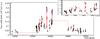 |
Fig. 1 Bayesian Blocks representation of the MAGIC light curve (black dots) from March 2007 to June 2009. The red dotted line defines the different identified blocks. The inlay shows a magnified version for the time range from December 2007 to June 2008, the high active Period 2. The long flat lines with no sampling between a data point and a new block do not guarantee a stable flux. |
In summary, during the three observation periods covered in this paper, Mrk 421 showed three clearly distinct VHE flux levels, with different apparent levels of variability. A quantitative evaluation of the VHE flux variability in these three periods is reported in Sects. 3 and 5, following the prescriptions given in Scargle (1998), Scargle et al. (2013) and Aleksić et al. (2015c).
3. Bayesian Blocks
We applied the Bayesian Block algorithm (Scargle 1998; Scargle et al. 2013) to the TeV light curve of Mrk 421. The algorithm generates a block-wise constant representation of a sequential data series by identifying statistically significant variations, and is suitable for characterizing local variability in astronomical light curves, even when not evenly sampled.
The optimal segmentation (defined by its change points) maximizes the goodness-of-fit with a certain model for the data lying in a block. The method requires a prior probability distribution parameter (ncpprior) for the number of changing points (Ncp), a kind of smoothing parameter derived from the assumption that Ncp ≪ N, the number of measurements. A false-positive rate (p0) is associated to the choice ncpprior.
The false-positive rate was chosen to be p0 = 0.01, leading to a ncpprior = 3.92. We obtained the 39 blocks representation for 95 data points shown as a red dotted line in Fig. 1 on top of the flux points measured by MAGIC (black dots). The height of each block is the weighted average of all integral fluxes belonging to it.
An advantage of the Bayesian Block algorithm is that it is able to identify significant changes in data series independently of variations in gaps or exposure. Therefore, no information on true or important flux changes is lost, as can happen when applying other techniques where the data series is binned in predefined temporal intervals.
Dates, factor of flux increase, and flux-doubling times of flares found by the Bayesian block algorithm for the MAGIC light curve.
This is the first time that the Bayesian Block algorithm has been applied to a VHE γ-ray light curve. We use the results to estimate the variability level of the light curve in the different observation periods and to define flares. To quantify the variability for each period, we can simply determine the ratio of resulting number of blocks and the number of data points. A higher ratio implies a higher flux variability. All six data points from Period 1 belong to the same initial block. This ratio of 1/6 indicates a low variability during this period. The lack of additional blocks during this period may also be related to the very low number of data points. The high activity in Period 2 is evident by the 30 blocks detected for 56 data points during this time period by the algorithm (see inlay of Fig. 1). The resulting ratio of 30/56, which is slightly above 0.5, shows that the light curve is substantially more variable than Period 1. In Period 3 we have an eight-block representation for 33 data points, which is a ratio of ~0.24. This lower variability of the light curve during this period shows a milder activity of the AGN than in Period 2. An additional discussion of the variability will be given in Sect. 5.
It is of great interest to identify flaring activities in light curves, but the definition of a flare is somewhat arbitrary and, since blazars vary on timescales from years down to minutes, a definition is strongly biased by the prejudice of the temporal bins used to produce the light curves. It is easy to miss flaring activities in light curves with too-large temporal bins (if the variability occurs on small timescales) or in light curves with too-small temporal bins (if the flux values are dominated by statistical uncertainties). In this context, the Bayesian Block algorithm benefits from a more suitable temporal split (according to the true variability), and hence it can be used as a very efficient method to find flares. In the following, VHE γ-ray flares are defined as a flux rise of at least a factor of two. This comparison is based on the block heights, that is the weighted average flux of all data points in one block. A flare can include several rising steps in a row, which add up to a local maximum in flux. Subsequently, the flux decreases to a lower flux, which can happen on a daily or longer timescale. By using this flux-doubling threshold we have been able to identify several flares, which are reported in Table 1.
We estimate the flux-doubling times using the height difference between consecutive blocks and the time between the last data point of a given block and the starting point of the next block, which is a conservative measure of the rise time between blocks. In the case of several consecutive flux rises among continuous blocks, the flux-doubling time reported in Table 1 considers the rise as a single increase from minimum to maximum. It can be seen that the flux doubles its value on different timescales. The flux-doubling can occur during just one night, for example for the block starting on MJD 54 502, but it can also take many days. Additionally, it should be noted that it cannot be ruled out that the flux might fall between two measurements. All determined flux-doubling times are subject to this possibility. For the first entry in the table the flux-doubling time of 139 days is not meaningful because the time interval includes the long observation gap from May to December 2007 where the source behaviour in γ-rays is unknown. Therefore, the flux-doubling times reported in Table 1 should be considered as upper limits to the actual time needed to double the flux. That is, the actual flux-doubling times could be shorter than the ones reported.
The flares identified using the Bayesian Block algorithm are marked in Fig. 2 by vertical dotted lines so that it is possible to compare these positions with features in the light curves in the other wavelengths.
4. Observations at X-ray, optical and radio wavelengths
To study the variability and correlation between the TeV γ-ray data and other wavebands, data from several other instruments were considered. In the X-ray range data from Swift/BAT and RXTE/ASM were selected. The optical data shown here is from the GASP-WEBT consortium (which includes data from the KVA telescope located at the ORM close to MAGIC). Data from the Metsähovi and OVRO telescopes are used in the radio range.
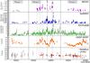 |
Fig. 2 Light curves of MAGIC, Swift/BAT, RXTE/ASM, GASP-WEBT, Metsähovi and OVRO from top to bottom in the time range from February 2007 to July 2009. The vertical dotted black lines denote the position of the TeV γ-ray flares as identified with the Bayesian Block algorithm (see Sect. 3). The vertical black lines mark the division between the three time periods (Period 1, Period 2, Period 3). |
4.1. Hard X-ray observations with Swift/BAT
The Burst Alert Telescope (BAT) on board the Swift satellite observes Mrk 421 in the hard X-ray regime, from 15 to 50 keV (Krimm et al. 2013). The Swift/BAT transient monitor results are provided by the Swift/BAT team2. Considering only averaged daily rates with a rate to rate error ratio greater than two, and additionally discarding six measurements with negative rates (on MJD 54 288, 54 476, 54 638, 54 750, 54 914, and 54 981), results in a total of 821 h of data distributed over 168 nightly flux measurements between 23rd February 2007 (MJD 54 154) and 17th June 2009 (MJD 54 999).
The Swift/BAT light curve of Mrk 421 is shown in Fig. 2. The overall hard X-ray flux behaviour is comparable to that of the MAGIC light curve, with a higher activity in Period 2 and several features that appear to be coincident, such as the peak structure around MJD 54 560.
4.2. Soft X-ray observations with RXTE/ASM
The all-sky monitor (ASM) was an instrument on board the RXTE satellite. It observed Mrk 421 in the energy range from 2 to 10 keV (Levine et al. 1996).
The results shown here are provided by the ASM/RXTE teams at MIT and at the RXTE SOF and GOF at NASA’s GSFC3. Only averaged daily count rates, each consisting of several so-called observation dwells of 90 s length, with a rate to rate error ratio greater than two are considered for the following studies. Additionally, two negative rates, on MJD 54 371 and 54 914, are discarded. This results in a total of 532 daily flux measurements with a total observation length of 260 h between 10th February 2007 (MJD 54 141) and 16th June 2009 (MJD 54 998).
The RXTE/ASM light curve of Mrk 421 is shown in Fig. 2. The soft X-ray flux shows a similar behaviour to that of the hard X-rays and VHE γ-rays, which includes several overall flux levels and peak structures that are present also in the Swift/BAT and MAGIC light curves.
4.3. Optical observations
The optical data in the R-band shown here were recorded by the KVA (Kungliga Vetenskapsakademien) telescope and a collection of telescopes, which work together in the GASP-WEBT (Whole Earth Blazar Telescope)4 consortium (Villata et al. 2008). The KVA telescope is situated at the ORM on La Palma close to the MAGIC telescopes. Photometric observations in the R-band are made with a 35 cm telescope. Observations are carried out in the same time intervals as MAGIC observations. Optical observations of Mrk 421 by the KVA telescope started in 2002, and show a variable optical light curve (Takalo et al. 2008).
Mrk 421 is regularly monitored by telecopes of GASP-WEBT, and KVA in particular. The optical data reported in this paper relate to the period from 18th February 2007 (MJD 54 149) to 23rd July 2009 (MJD 55 035), which were recorded by the following instruments: Abastumani, Castelgrande, Crimean, L’Ampolla, Lulin, KVA, New Mexico Skies (now called iTelescopes), Sabadell, St. Petersburg, Talmassons, Torino, and Tuorla observatories. It should be mentioned that the flux measurements are corrected for the contribution of the host galaxy (see Nilsson et al. 2007) as well as for galactic extinction (Schlafly & Finkbeiner 2011).
The GASP-WEBT light curve shown in Fig. 2 includes a total of 815 observations distributed over 353 nights. When comparing the optical light curve to the γ-ray and X-ray light curves it is important to note that the optical light curve cannot be separated into different activity phases as the other light curves can be. The flux varies by the same amount throughout the whole observation length of more than two years. It can be seen that the features in the GASP-WEBT light curve are longer than and not coincident with those of the MAGIC, RXTE/ASM and Swift/BAT light curves.
4.4. Radio observations with Metsähovi
Radio data at 37 GHz are recorded by the 13.7 m telescope at the Metsähovi Radio Observatory in Finland (Teräsranta et al. 1998).
Considering only data points with a flux to error ratio greater than four of the Metsähovi light curve, leaves 49 nightly flux measurements between 13th February 2007 (MJD 54 144) and 24th June 2009 (MJD 55 006). The light curve is shown in Fig. 2. In comparison to the VHE γ-ray, the X-ray and the optical light curves mentioned above, the overall radio flux measured by Metsähovi is rather stable, yet with a slight decrease in Period 3.
4.5. Radio observations with OVRO
The Owens Valley Radio Observatory (OVRO), located in the USA, operates a 40 m radio telescope measuring at 15 GHz. It started observations in January 2008 and therefore does not cover the whole time span of MAGIC observations5 (Richards et al. 2011).
In the available data set, often two observations were made during one day, which were only separated by ~2 min. These data points were averaged, which results in a total of 119 data points. The light curve with data points between 8th January 2008 (MJD 54 473) and 8th June 2009 (MJD 54 990) is shown in Fig. 2. As it occurs with the Metsähovi light curve, the flux is rather stable, with a small decrease in Period 3.
5. Multi-band flux variability
In order to quantify the variability in the emission of Mrk 421, the fractional variability Fvar, as it is given in Eq. (10) in Vaughan et al. (2003), is used. It is calculated using 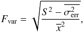 (1)and represents the normalized excess variance. S is the standard deviation and
  the mean square error of the flux measurements.
  stands for the average flux. The uncertainty of Fvar is given by Eq. (2) in Aleksić et al. (2015c), after Poutanen et al. (2008):
 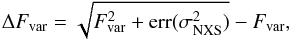 (2)where
  is given by Eq. (11) of Vaughan et al. (2003):
 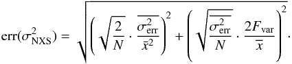 (3)Here, N is the number of data points in a light curve. Note from Eq. (1) that Fvar is not defined (and hence cannot be used) when the excess variance is negative, which can occur in the absence of variability, or when the instrument sensitivity is not good enough to detect it (i.e. large flux uncertainties).
Fvar is calculated for all the light curves shown in Fig. 2 and the results are shown in Fig. 3 with open markers. For MAGIC, Swift/BAT, RXTE/ASM, Metsähovi and OVRO, the shown light curves feature one data point per night. For GASP-WEBT, the light curve contains nights with more than one data point. For the calculation of Fvar, the multiple GASP-WEBT optical fluxes related to single days were averaged, thus obtaining a single value.
In order to improve the direct comparison of the variability determined for the various energy bands, we also computed Fvar using only the multi-instrument observations that are strictly simultaneous to those performed by MAGIC. These Fvar values are depicted by the filled markers in Fig. 3, and remove potential biases due to the somewhat different temporal coverage of the various instruments.
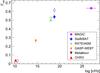 |
Fig. 3 Fractional variability (Fvar) as a function of the frequency for the 2.3 yr long time range from February 2007 to July 2009. The fractional variability was computed in two different ways: using all the flux measurements from the light curves reported in Fig. 2 (depicted with open markers), and using only those observations simultaneous to the VHE γ-ray measurements from MAGIC (depicted with filled markers). Vertical bars denote 1σ uncertainties and horizontal bars indicate the width of each energy bin. |
The overall behaviour of the fractional variability shows a rising tendency with increasing frequency. Considering only the Fvar values determined with simultaneous multi-instrument observations (filled markers in Fig. 3), the highest variability occurs in the VHE γ-ray band measured by MAGIC (Fvar = 0.64 ± 0.01), although it is quite similar to the variability measured in the soft X-ray band (Fvar = 0.50 ± 0.01) and hard X-ray band (Fvar = 0.54 + ± 0.02) by RXTE/ASM and Swift/BAT respectively.
As mentioned in the previous sections (e.g. see Fig. 2), the overall flux levels and source activity appear different for the three different observation periods. Figure 4 reports the multi-band fractional variability determined separately for Periods 1, 2 and 3. The main trend observed in the 2.3 yr long time span reported in Fig. 3 is also reproduced when splitting the data in the three different periods: Fvar always increases with energy, with the highest variability occurring in the X-ray and VHE γ-ray bands. The Swift/BAT light curve with one-day temporal bins reported in Fig. 2 has large statistical uncertainties, that, because of the relatively low activity and low variability of Mrk 421 during Periods 1 and 3, yielded a negative excess variance, hence preventing the calculation of the fractional variability for these two periods. On the other hand, the RXTE/ASM light curve with one-day temporal bins reported in Fig. 2 have somewhat smaller uncertainties and a better temporal coverage than that of Swift/BAT, which permitted the quantification of the fractional variability in the soft X-ray energy band for the three temporal periods considered.
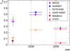 |
Fig. 4 Multi-instrument fractional variability (Fvar) for the three periods defined in Fig. 2. The fractional variability was computed using only those observations simultaneous to the VHE γ-ray measurements from MAGIC. Vertical bars denote 1σ uncertainties and horizontal bars indicate the covered time span of each instrument. |
In Fig. 4 it can also be seen that the variability for the MAGIC light curve is higher for Period 2 than in Periods 1 and 3 as it was already shown by the quantification of the variability with the results of the Bayesian Block algorithm (see Sect. 3). Due to the lower average flux in Period 1 compared to Period 3, the fractional variability in Period 1 is higher than in Period 3.
It is worth noticing that the fractional variability in the optical band is comparable to that at X-rays and VHE γ-rays during Period 3, which did not happen during Periods 1 and 2. Inspecting the light curves reported in Fig. 2, one can see that the timescales involved in the reported variabilities are very different. While the X-ray and VHE γ-ray light curves show day-long flux variations on the top of a rather stable flux level, the optical flux shows many-day-long flux variations on the top of a flux level that increases by about a factor of two throughout Period 3. Therefore, despite the very comparable Fvar values during Period 3, the emission in the optical band is probably not related to that in the X-ray and VHE γ-ray bands.
These results are consistent with results from previous publications. This includes the rising fractional variability of Mrk 421 from optical to X-ray energies in 2001 (Giebels et al. 2007) and the same increase from optical to X-ray energies in March 2010 during a flare with a comparable variability of the VHE and the X-ray light curves (Aleksić et al. 2015b). These results are complemented by Aleksić et al. (2015a) and Baloković et al. (2016), which presented multi-wavelength data during the relatively low activity observed from January to June 2009 and from January to March 2013 respectively. These include results from the Fermi-LAT closing the gap between the X-ray and TeV γ-ray energy bands. They report a low flux in radio energies, rising to a maximum in the X-ray energy band. For GeV γ-rays measured by the Fermi-LAT the variability drops to a level comparable to the optical and UV wave band. The variability in the TeV γ-ray light curves increases to a level comparable to X-rays, which is consistent with the result from this study, that uses a much larger time span.
6. Multi-band correlations
To quantify the correlation of two light curves, the discrete correlation function (DCF), which was introduced by Edelson & Krolik (1988), is used here. A study of the correlations of the MAGIC light curve with light curves of other wavelengths has already been carried out for Mrk 421 for the first half of 2009 in Aleksić et al. (2015a). In that publication a method to determine confidence intervals for the resulting correlation is described in detail. Here, a short introduction to the method will be given. For more detailed information on that method the reader is referred to the cited publication and references therein.
The errors of the DCF values as stated by Edelson & Krolik (1988) might not be appropriate when the individual light-curve data points are correlated red-noise data (Uttley et al. 2003). Red-noise data are characterized by a power spectral density per unit of bandwidth proportional to 1/f2, where f is the frequency (Chatterjee et al. 2012). Since this is not the case for the given light curves, a Monte Carlo based approach is applied here to determine confidence intervals for the DCF values. Therefore, 1000 light curves are simulated for each telescope which feature the same sampling pattern and comparable exposure times as the original light curve. In addition, the power spectral density (PSD) should be as similar as possible to the PSD of the original light curve. Therefore, the light curves are simulated with PSDs following a power law with spectral indices in a range from −1.0 to −2.9 in steps of 0.1. The light curves with the PSD which match the PSD of the original light curve best, are determined using the PSRESP method (Chatterjee et al. 2008).
The DCF itself is calculated for sets of original light curves. With the calculated DCF of 1000 simulated light curves of one telescope and the original light curve of a second telescope, finally the confidence bands can be determined. Here, the confidence limits are determined as the 1%, 5%, 95% and 99% quantiles of the 1000 resulting DCFs.
In the following plots, the black dots and error bars are the DCF and its error calculated after Edelson & Krolik (1988). The blue and green lines represent the confidence limits of 95% and 5% and of 99% and 1% respectively determined with DCFs of the 1000 simulated light curves of the first telescope and the original light curve of the second telescope. A value above the 99% confidence limit is considered as a significant correlation, a significant anti-correlation is given for a value below the 1% limit.
A binning of two days is chosen in this case. The reason for this is the unequal binning of the light curves which might lead to shifts in the correlations by one day when the time difference in the two light curves is larger than half a day. Time lags between − 50 and +50 days are examined. The time lag Δt is defined as the time difference of the second light curve to the first light curve (Instrument1 vs. Instrument2).
In the following subsections we report the results from our study on the correlation between the optical, X-ray and VHE γ-ray bands. The radio bands do not show significant variability and hence the radio fluxes cannot be correlated to the fluxes in the other bands.
6.1. RXTE/ASM and MAGIC
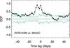 |
Fig. 5 Discrete correlation function for the light curves of RXTE/ASM and MAGIC for the 2.3 yr long period (Period 1, 2 and 3). Time lags from −50 to +50 days in steps of two days are considered. Black dots represent the DCF values with the error bars calculated as in Edelson & Krolik (1988). The green (blue) lines represent the 99% and 1% (95% and 5%) confidence limits for random correlations resulting from the dedicated Monte Carlo analysis described in Sect. 6. |
The RXTE/ASM and MAGIC cross-correlations were examined at first for the whole time range from February 2007 to June 2009. This is reported in Fig. 5.
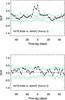 |
Fig. 6 Discrete correlation function for the light curves of RXTE/ASM and MAGIC for Period 2 (top) and for Period 3 (bottom). The description of data points and contours are given in the caption of Fig. 5. |
There is positive and significant correlation for the entire range of time lags considered, that is from − 50 to +50 days. The main cause of this positive correlation is the substantially larger flux level in Period 2, compared with that in Periods 1 and 3. If the light curves are shifted by a time lag smaller than the duration of these periods (e.g. 50 days), the pairing of VHE γ-ray fluxes and X-ray fluxes occurs always (for all time lags) within the observations from the same period, and hence one gets high VHE flux values related to high X-ray flux values, that is all from Period 2, and low VHE flux values matched with low X-ray flux values, that is all from Periods 1 and 3. And this effect naturally produces a positive correlation.
To remove the effect of the substantially different flux levels between the different periods, as well as to test the influence of the different states of activity and flux strength reported in the previous sections, the DCF is determined separately for Periods 2 and 3. The MAGIC light curve in the quiet Period 1 contains only six data points and is therefore not included in this study. The results are shown in Fig. 6. We note that there is still an overall positive correlation for both Periods 2 and 3, however the DCF values are typically within the 95% confidence contours. This positive (but not significant) correlation for all time lags is due to the fact that the two light curves considered here have the same overall trends: in Period 2 the VHE γ-ray and the X-ray light curves show an overall flux increase throughout the entire period, whereas in Period 3 they both show an overall decrease.
The quiet Period 3 shows a marginally significant correlation around a time lag of zero, while the active Period 2 shows a prominent correlation, with some structure around a time lag of zero. The DCF structure depicted in the top panel of Fig. 6 resembles that in Fig. 5, which indicates that the correlations in the high-activity Period 2 dominate the DCF values reported in Fig. 5, that relate to the full 2.3 yr time interval. In both cases, one finds a peak at Δt = 0 and Δt = − 6 days. The first peak is due to the direct correlation dominated by simultaneous prominent features in both light curves (i.e. flares on MJD 54 556 and 54 622). On the other hand, the DCF peak at − 6 days is dominated by the remarkable three-day long X-ray flaring activity around MJD 54 630, which is the highest flux value in the RXTE/ASM light curve. There is no counterpart in the VHE γ-ray light curve because MAGIC did not observe around that date, but this prominent X-ray flaring activity is matched with the large VHE flaring activity around MJD 54 622 for time lags of around − 6 days. The relatively broad structure of positive DCF values, extending from − 10 days to +6 days, is dominated by the remarkable and asymmetric flaring activity in the X-ray light curve in a broad region around MJD 54 556, which is coindicent with the relatively short VHE flare at the same location.
6.2. Swift/BAT and MAGIC
The sensitivity and temporal coverage of Swift/BAT is somewhat lower than that of RXTE/ASM, which reduces the accuracy with which one can study the correlation between the hard X-ray band above 15 keV and the VHE γ-rays. For Period 3, we could only find a marginally significant correlation dominated by the somewhat higher X-ray and VHE flux values in the MJD range from 54 858 to 54 864. In Fig. 7 the correlation results of the Swift/BAT and the MAGIC light curves in the high-activity Period 2 are shown. When considering this period, we find DCF values above the 95% confidence level for time lags between − 8 days and +2 days, with two peaks above the 99% confidence level for the time lags of 0, and also − 8 and − 6 days. The explanation of these two peaks is essentially the same as was given for the correlations between RXTE/ASM and MAGIC reported in Sect. 6.1. The peak at Δt = 0 is dominated by several features appearing simultaneously in both light curves, the peak at − 6 to − 8 days is dominated by the large three-day long X-ray activity around MJD 54 630 (where we do not have MAGIC observations), and the broad and somewhat asymmetric structure in the DCF plot is dominated by the large and broad and asymmetric X-ray flaring around MJD 54 556.
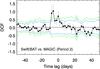 |
Fig. 7 Discrete correlation function for the light curves of Swift/BAT and MAGIC for Period 2. The description of data points and contours are given in the caption of Fig. 5. |
6.3. GASP-WEBT and MAGIC
The correlation between the GASP-WEBT and MAGIC light curve for the high-activity Period 2 is shown in Fig. 8. There is a positive correlation for time lags between 0 and +28 days, as well as around − 44 days, and a negative correlation for time lags around − 28 and around +44 days. This alternation of correlation and anti-correlation is caused by the fact that the variability in the optical and VHE emission is dominated by two to three prominent features. And hence the alternating presence of rises and drops in flux in both light curves creates these features in the DCF. For instance, when shifting the optical light curve by e.g. +24 days or − 44 days, minima and maxima in the two light curves become aligned yielding a significant correlation, while when the optical light curve is shifted by − 28 or +44 days, the minima in one light curve are aligned with maxima in the other light curve, hence yielding a significant anti-correlation. Although the reported correlations for some time lags are significant from the statistical point of view, they are based on the alignment or misalignment of only two to three prominent and relatively broad features, and these prominent features are not necessarily related to each other.
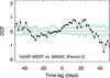 |
Fig. 8 Discrete correlation function for the light curves of GASP-WEBT and MAGIC for Period 2. The description of data points and contours are given in the caption of Fig. 5. |
In the quiet Period 3, we find an overall anti-correlation during the entire range of time lags proved. This result is produced by the overall flux decrease in the VHE light curve and the overall flux increase in the optical light curve throughout the entire Period 3. The same result was reported and discussed in Aleksić et al. (2015a).
6.4. GASP-WEBT and RXTE/ASM
The DCF results of GASP-WEBT and RXTE/ASM in Period 2 are shown in Fig. 9. A correlation is seen for positive time lags between +6 and +30 days, as well as for negative time lags between − 50 and − 38 days. Anti-correlations are seen between − 28 and − 10 days and between +44 and +50 days. These results are comparable to the results between GASP-WEBT and MAGIC. This again shows the alternation of rises and drops in flux produced by the fact that the variability in the optical and X-ray emission is dominated by only two to three prominent features. When shifting the optical light curve by the time lags, for which correlations are found, maxima in both light curves are aligned. When shifting the light curve by the time lags, for which anti-correlations are found, minima in the optical light curve are aligned with maxima in the X-ray light curves. Again, these correlations and anti-correlations might have been found by chance.
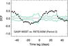 |
Fig. 9 Discrete correlation function for the light curves of GASP-WEBT and RXTE/ASM for Period 2. The description of data points and contours are given in the caption of Fig. 5. |
In Period 1 no correlations nor anti-correlations are seen for this pair of instruments. However, in Period 3 the GASP-WEBT light curve shows an overall anti-correlation with the RXTE/ASM light curve, which occurs due to the overall slow decrease of the X-ray rate and the flux increase in the optical light curve. This result is comparable to the overall anti-correlation for the X-ray and TeV γ-ray light curves discussed in Aleksić et al. (2015a), which used a part of the data set used in this paper.
7. Summary of results
-
1.
Between March 2007 and June 2009, MAGIC-I accumulated 96 h of VHE γ-ray data of the blazar Mrk 421: the VHE flux varied around the typical flux baseline of about 0.5 CU, with the highest flux of about 3.8 CU occurring during the active state in 2008.
-
2.
For the first time the Bayesian Block algorithm was applied to the VHE γ-ray light curve from a Cherenkov telescope to identify different flux emission states, as well as to quantify the variability and to search for flaring activity.
-
3.
The MAGIC γ-ray light curve was compared to light curves of other wavebands, including the hard and soft X-ray wavebands from SwiftBAT and RXTE/ASM, the optical R-band from GASP-WEBT, and two radio wavebands from Metsähovi and OVRO.
-
4.
The VHE and X-ray light curves resemble each other, showing a number of few-day long structures, while the optical and radio light curves show smaller flux variations and occurring on longer timescales.
-
5.
The fractional variability is low for radio and optical wavebands, and high for the X-ray and VHE γ-ray bands during both low and high activity.
-
6.
The discrete correlation function shows a direct relation between the two X-ray bands and the VHE γ-ray band, while no correlation was found between the optical and the X-ray and VHE bands.
8. Discussion and conclusions
We have peformed a comprehensive variability and correlation study with 2.3 yr of multi-band data from Mrk 421. The measured variability as a function of energy, with the highest variability in the X-ray and VHE bands, and the observed direct X-ray-to-VHE correlation, both occuring comparably during high- and low-activity, suggests that the processes that dominate the flux variability in Mrk 421 are similar for the different activity levels. The pattern characterized by a high variability in the X-ray and γ-ray emission, accompanied by a low variability in the optical and radio emission, occurs in both quiescent and excited states, qualifying this behaviour as typical of Mrk 421. The low variability and different timescales observed both in the radio and optical emission may be explained by different emission regions, or by cooler electrons in the jet at a later time. Additionally, the correlation between the X-ray and the VHE γ-ray emission extending over many months suggests that the broadband emission of Mrk 421 is predominantly produced by the same particles, for example via the SSC process. Alternatively, the X-rays and γ-rays could both result from the same radiation process (e.g. synchrotron radiation), but from two different electron populations varying together most of the time, but not necessarily always. This is the case in hadronic scenarios where the X-ray and γ-ray photons result from the synchrotron radiation of electrons in subsequent and therefore coupled cascade generations (Mannheim 1993). The cascade generations are driven by the pair production in photon-photon scatterings involving low-energy photon fields, which can vary themselves, thereby modulating the variations of flux of the primary photo-mesons at the top of the cascades.
A Crab unit is defined here as a flux of 8.08 × 10⁻¹¹ cm-2 s-1 in the energy range from 400 GeV to 50 TeV (Albert et al. 2008).
Acknowledgments
We would like to thank the Instituto de Astrofísica de Canarias for the excellent working conditions at the Observatorio del Roque de los Muchachos in La Palma. The financial support of the German BMBF and MPG, the Italian INFN and INAF, the Swiss National Fund SNF, the ERDF under the Spanish MINECO (FPA2012-39502), and the Japanese JSPS and MEXT is gratefully acknowledged. This work was also supported by the Centro de Excelencia Severo Ochoa SEV-2012-0234, CPAN CSD2007-00042, and MultiDark CSD2009-00064 projects of the Spanish Consolider-Ingenio 2010 programme, by grant 268740 of the Academy of Finland, by the Croatian Science Foundation (HrZZ) Project 09/176 and the University of Rijeka Project 13.12.1.3.02, by the DFG Collaborative Research Centers SFB823/C4 and SFB876/C3, and by the Polish MNiSzW grant 745/N-HESS-MAGIC/2010/0. The public data archives of Swift/BAT and RXTE/ASM are acknowledged. We thank the OVRO telescope for making its results available for the public. The OVRO 40 m monitoring program is supported in part by NASA grants NNX08AW31G and NNX11A043G, and NFS grants AST-0808050 and AST-1109911. We also thank the KVA and Metsähovi telescopes for making their light curves available. M. Villata organized the optical-to-radio observations by GASP-WEBT as the president of the collaboration. The Metsähovi team acknowledges the support from the Academy of Finland to our observing projects (numbers 212656, 210338, 121148, and others). St. Petersburg University team acknowledges support from Russian RFBR grant 15-02-00949 and St. Petersburg University research grant 6.38.335.2015. The Abastumani Observatory team acknowledges financial support by the Shota Rustaveli National Science Foundation under contract FR/577/6-320/13.
References
- Abdo, A. A., Ackermann, M., Ajello, M., et al. 2011, ApJ, 736, 131 [NASA ADS] [CrossRef] [Google Scholar]
- Acciari, V. A., Aliu, E., Aune, T., et al. 2009, ApJ, 703, 169 [NASA ADS] [CrossRef] [Google Scholar]
- Acciari, V. A., Aliu, E., Arlen, T., et al. 2011, ApJ, 738, 25 [NASA ADS] [CrossRef] [Google Scholar]
- Acciari, V. A., Arlen, T., Aune, T., et al. 2014, Astropart. Phys., 54, 1 [NASA ADS] [CrossRef] [Google Scholar]
- Albert, J., Aliu, E., Anderhub, H., et al. 2007, ApJ, 663, 125 [NASA ADS] [CrossRef] [Google Scholar]
- Albert, J., Aliu, E., Anderhub, H., et al. 2008, ApJ, 674, 1037 [NASA ADS] [CrossRef] [Google Scholar]
- Aleksić, J., Alvarez, E. A., Antonelli, L. A., et al. 2012, A&A, 542, A100 [NASA ADS] [CrossRef] [EDP Sciences] [Google Scholar]
- Aleksić, J., Ansoldi, S., Antonelli, L. A., et al. 2015a, A&A, 576, A126 [NASA ADS] [CrossRef] [EDP Sciences] [Google Scholar]
- Aleksić, J., Ansoldi, S., Antonelli, L. A., et al. 2015b, A&A, 578, A22 [NASA ADS] [CrossRef] [EDP Sciences] [Google Scholar]
- Aleksić, J., Ansoldi, S., Antonelli, L. A., et al. 2015c, A&A, 573, A50 [NASA ADS] [CrossRef] [EDP Sciences] [Google Scholar]
- Aleksić, J., Ansoldi, S., Antonelli, L. A., et al. 2016a, Astropart. Phys., 72, 61 [NASA ADS] [CrossRef] [Google Scholar]
- Aleksić, J., Ansoldi, S., Antonelli, L. A., et al. 2016b, Astropart. Phys., 72, 76 [NASA ADS] [CrossRef] [Google Scholar]
- Aliu, E., Anderhub, H., Antonelli, L. A., et al. 2009, Astropart. Phys., 30, 293 [NASA ADS] [CrossRef] [Google Scholar]
- Baloković, M., Paneque, D., Madejski, G., et al. 2016, ApJ, 819, 156 [NASA ADS] [CrossRef] [Google Scholar]
- Bartoli, B., Bernardini, P., Bi, X. J., et al. 2011, ApJ, 734, 110 [NASA ADS] [CrossRef] [Google Scholar]
- Błażejowski, M., Blaylock, G., Bond, I. H., et al. 2005, ApJ, 630, 130 [NASA ADS] [CrossRef] [Google Scholar]
- Buckley, J. H., Akerlof, C. W., Biller, S., et al. 1996, ApJ, 472, L9 [NASA ADS] [CrossRef] [Google Scholar]
- Cao, G., & Wang, J. 2013, PASJ, 65, 109 [NASA ADS] [CrossRef] [Google Scholar]
- Chatterjee, R., Jorstad, S. G., Marscher, A. P., et al. 2008, ApJ, 689, 79 [NASA ADS] [CrossRef] [Google Scholar]
- Chatterjee, R., Bailyn, C. D., Bonning, E. W., et al. 2012, ApJ, 749, 191 [NASA ADS] [CrossRef] [Google Scholar]
- Cui, W. 2004, ApJ, 605, 662 [NASA ADS] [CrossRef] [Google Scholar]
- Donnarumma, I., Vittorini, V., Vercellone, S., et al. 2009, ApJ, 691, L13 [NASA ADS] [CrossRef] [Google Scholar]
- Edelson, R. A., & Krolik, J. H. 1988, ApJ, 333, 646 [NASA ADS] [CrossRef] [Google Scholar]
- Fomin, V. P., Stepanian, A. A., Lamb, R. C., et al. 1994, Astropart. Phys., 2, 137 [NASA ADS] [CrossRef] [Google Scholar]
- Fossati, G., Buckley, J., Edelson, R. A., Horns, D., & Jordan, M. 2004, New Astron., 48, 419 [Google Scholar]
- Fossati, G., Buckley, J. H., Bond, I. H., et al. 2008, ApJ, 677, 906 [NASA ADS] [CrossRef] [Google Scholar]
- Gaidos, J. A., Akerlof, C. W., Biller, S., et al. 1996, Nature, 383, 319 [NASA ADS] [CrossRef] [Google Scholar]
- Giebels, B., Dubus, G., & Khélifi, B. 2007, A&A, 462, 29 [NASA ADS] [CrossRef] [EDP Sciences] [Google Scholar]
- Horan, D., Acciari, V. A., Bradbury, S. M., et al. 2009, ApJ, 695, 596 [NASA ADS] [CrossRef] [Google Scholar]
- Hovatta, T., Petropoulou, M., Richards, J. L., et al. 2015, MNRAS, 448, 3121 [NASA ADS] [CrossRef] [Google Scholar]
- Katarzyński, K., Sol, H., & Kus, A. 2003, A&A, 410, 101 [NASA ADS] [CrossRef] [EDP Sciences] [Google Scholar]
- Krimm, H. A., Holland, S. T., Corbet, R. H. D., et al. 2013, ApJS, 209, 14 [NASA ADS] [CrossRef] [Google Scholar]
- Levine, A. M., Bradt, H., Cui, W., et al. 1996, ApJ, 469, L33 [NASA ADS] [CrossRef] [Google Scholar]
- Lico, R., Giroletti, M., Orienti, M., et al. 2014, A&A, 571, A54 [NASA ADS] [CrossRef] [EDP Sciences] [Google Scholar]
- Macomb, D. J., Akerlof, C. W., Aller, H. D., et al. 1995, ApJ, 449, L99 [NASA ADS] [CrossRef] [Google Scholar]
- Mannheim, K. 1993, A&A, 269, 67 [NASA ADS] [Google Scholar]
- Max-Moerbeck, W., Hovatta, T., Richards, J. L., et al. 2014, MNRAS, 445, 428 [NASA ADS] [CrossRef] [Google Scholar]
- Nilsson, K., Pasanen, M., Takalo, L. O., et al. 2007, A&A, 475, 199 [NASA ADS] [CrossRef] [EDP Sciences] [Google Scholar]
- Piner, B. G., Unwin, S. C., Wehrle, A. E., et al. 1999, ApJ, 525, 176 [NASA ADS] [CrossRef] [Google Scholar]
- Poutanen, J., Zdziarski, A. A., & Ibragimov, A. 2008, MNRAS, 389, 1427 [NASA ADS] [CrossRef] [Google Scholar]
- Punch, M., Akerlof, C. W., Cawley, M. F., et al. 1992, Nature, 358, 477 [NASA ADS] [CrossRef] [Google Scholar]
- Richards, J. L., Max-Moerbeck, W., Pavlidou, V., et al. 2011, ApJS, 194, 29 [NASA ADS] [CrossRef] [Google Scholar]
- Scargle, J. D. 1998, ApJ, 504, 405 [NASA ADS] [CrossRef] [Google Scholar]
- Scargle, J. D., Norris, J. P., Jackson, B., & Chiang, J. 2013, ApJ, 764, 167 [NASA ADS] [CrossRef] [Google Scholar]
- Schlafly, E. F., & Finkbeiner, D. P. 2011, ApJ, 737, 103 [NASA ADS] [CrossRef] [Google Scholar]
- Takalo, L. O., Nilsson, K., Lindfors, E., et al. 2008, in AIP Conf. Ser. 1085, eds. F. A. Aharonian, W. Hofmann, & F. Rieger, 705 [Google Scholar]
- Teräsranta, H., Tornikoski, M., Mujunen, A., et al. 1998, A&AS, 132, 305 [NASA ADS] [CrossRef] [EDP Sciences] [Google Scholar]
- Tluczykont, M., Bernardini, E., Satalecka, K., et al. 2010, A&A, 524, A48 [NASA ADS] [CrossRef] [EDP Sciences] [Google Scholar]
- Uttley, P., Edelson, R., McHardy, I. M., Peterson, B. M., & Markowitz, A. 2003, ApJ, 584, L53 [NASA ADS] [CrossRef] [Google Scholar]
- Vaughan, S., Edelson, R., Warwick, R. S., & Uttley, P. 2003, MNRAS, 345, 1271 [NASA ADS] [CrossRef] [Google Scholar]
- Villata, M., Raiteri, C. M., Larionov, V. M., et al. 2008, A&A, 481, L79 [NASA ADS] [CrossRef] [EDP Sciences] [Google Scholar]
- Zanin, R., Carmona, E., Sitarek, J., et al. 2013, in Proc. 33rd International Cosmic Ray Conference (Rio de Janeiro, Brazil) [Google Scholar]
All Tables
Dates, factor of flux increase, and flux-doubling times of flares found by the Bayesian block algorithm for the MAGIC light curve.
All Figures
|
Fig. 1 Bayesian Blocks representation of the MAGIC light curve (black dots) from March 2007 to June 2009. The red dotted line defines the different identified blocks. The inlay shows a magnified version for the time range from December 2007 to June 2008, the high active Period 2. The long flat lines with no sampling between a data point and a new block do not guarantee a stable flux. |
| In the text | |
|
Fig. 2 Light curves of MAGIC, Swift/BAT, RXTE/ASM, GASP-WEBT, Metsähovi and OVRO from top to bottom in the time range from February 2007 to July 2009. The vertical dotted black lines denote the position of the TeV γ-ray flares as identified with the Bayesian Block algorithm (see Sect. 3). The vertical black lines mark the division between the three time periods (Period 1, Period 2, Period 3). |
| In the text | |
|
Fig. 3 Fractional variability (Fvar) as a function of the frequency for the 2.3 yr long time range from February 2007 to July 2009. The fractional variability was computed in two different ways: using all the flux measurements from the light curves reported in Fig. 2 (depicted with open markers), and using only those observations simultaneous to the VHE γ-ray measurements from MAGIC (depicted with filled markers). Vertical bars denote 1σ uncertainties and horizontal bars indicate the width of each energy bin. |
| In the text | |
|
Fig. 4 Multi-instrument fractional variability (Fvar) for the three periods defined in Fig. 2. The fractional variability was computed using only those observations simultaneous to the VHE γ-ray measurements from MAGIC. Vertical bars denote 1σ uncertainties and horizontal bars indicate the covered time span of each instrument. |
| In the text | |
|
Fig. 5 Discrete correlation function for the light curves of RXTE/ASM and MAGIC for the 2.3 yr long period (Period 1, 2 and 3). Time lags from −50 to +50 days in steps of two days are considered. Black dots represent the DCF values with the error bars calculated as in Edelson & Krolik (1988). The green (blue) lines represent the 99% and 1% (95% and 5%) confidence limits for random correlations resulting from the dedicated Monte Carlo analysis described in Sect. 6. |
| In the text | |
|
Fig. 6 Discrete correlation function for the light curves of RXTE/ASM and MAGIC for Period 2 (top) and for Period 3 (bottom). The description of data points and contours are given in the caption of Fig. 5. |
| In the text | |
|
Fig. 7 Discrete correlation function for the light curves of Swift/BAT and MAGIC for Period 2. The description of data points and contours are given in the caption of Fig. 5. |
| In the text | |
|
Fig. 8 Discrete correlation function for the light curves of GASP-WEBT and MAGIC for Period 2. The description of data points and contours are given in the caption of Fig. 5. |
| In the text | |
|
Fig. 9 Discrete correlation function for the light curves of GASP-WEBT and RXTE/ASM for Period 2. The description of data points and contours are given in the caption of Fig. 5. |
| In the text | |
Current usage metrics show cumulative count of Article Views (full-text article views including HTML views, PDF and ePub downloads, according to the available data) and Abstracts Views on Vision4Press platform.
Data correspond to usage on the plateform after 2015. The current usage metrics is available 48-96 hours after online publication and is updated daily on week days.
Initial download of the metrics may take a while.