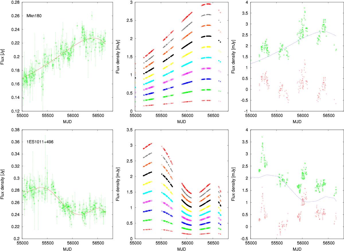
Three steps to estimate the contribution from the slowly varying component to the optical light curves for Mkn 180 (top) 1ES 1011+496 (bottom). Left: the polynomial (red solid line) is fit to the radio light curve (green symbols). Middle: the polynomial is scaled to the same average flux density as the optical light curve and then multiplied with 0.1 (red crosses), 0.2, 0.3, ... 1.0 (red triangles). These polynomial-multiples are subtracted from the optical light curve. Right: the optical light curve from which the polynomial-multiple that minimizes the rms (blue line, 0.9 for Mkn 180 and 0.7 for 1ES 1011+496) has been subtracted (red) and the original optical data (green).