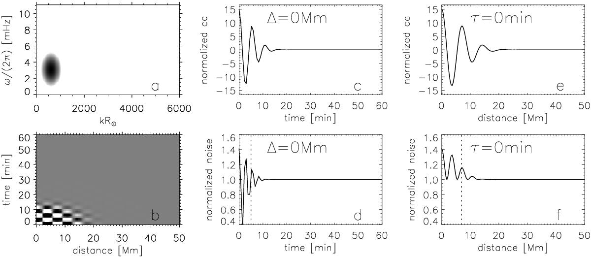
Examples of the power spectrum in logarithmic gray scale (Panel a)) and the expectation value of the cross-covariance function (Panel b)) in the case of the Gaussian power spectrum. In Panel a) (and the same is true in Figs. 2a and 4a), larger and smaller power is indicated by black and white, respectively. The peak of the power is located at (k₀R_⊙,ω₀/ (2π)) = (600,3 mHz) and the peak has widths (σ_kR_⊙,σ_ω/ (2π)) = (100,0.5 mHz). The cuts through the expectation value of the cross-covariance function at Δ = 0 and τ = 0 are shown in Panels c) and e), and the noise for the same cuts are shown in Panels d) and f). The cross-covariance (cc) function and the noise, , are both normalized by . This choice of normalization means that the amplitude of the cross-covariance function directly gives the signal-to-noise ratio (E [C(Δ,τ)] /σ(0,0)). The vertical dotted lines in Panels d) and f) indicate the expected width of the noise in time and space, 5 min and 7 Mm, respectively.