| Issue |
A&A
Volume 593, September 2016
|
|
|---|---|---|
| Article Number | A43 | |
| Number of page(s) | 8 | |
| Section | Extragalactic astronomy | |
| DOI | https://doi.org/10.1051/0004-6361/201628120 | |
| Published online | 12 September 2016 | |
The ionization rates of galactic nuclei and disks from Herschel/HIFI observations of water and its associated ions⋆
1 SRON Netherlands Institute for Space
Research, Landleven
12, 9747
AD Groningen, The Netherlands
e-mail: This email address is being protected from spambots. You need JavaScript enabled to view it.
2 Kapteyn Astronomical Institute,
University of Groningen, 9700
AV
Groningen, The
Netherlands
3 Max-Planck-Institut für
Radioastronomie, Auf dem Hügel
69, 53121
Bonn,
Germany
Received:
13
January
2016
Accepted:
15
June
2016
Abstract
Context. Dense gas in galactic nuclei is known to feed central starbursts and AGN, but the properties of this gas are poorly known because of the high obscuration by dust.
Aims. Submm-wave spectroscopy of water and its associated ions is useful to trace the oxygen chemistry of interstellar gas, in particular to constrain its ionization rate.
Methods. We present Herschel/HIFI spectra of the H2O 1113 GHz and H2O+ 1115 GHz lines toward five nearby prototypical starburst/AGN systems, and OH+ 971 GHz spectra toward three of these. The beam size of 20′′ corresponds to resolutions between 0.35 and 7 kpc.
Results. The observed line profiles range from pure absorption (NGC 4945, M 82) to P Cygni indicating outflow (NGC 253, Arp 220) and inverse P Cygni indicating infall (Cen A). The similarity of the H2O, OH+, and H2O+ profiles to each other and to HI indicates that diffuse and dense gas phases are well mixed. We estimate column densities assuming negligible excitation (for absorption features) and using a non-LTE model (for emission features), adopting calculated collision data for H2O and OH+, and rough estimates for H2O+. Column densities range from ~1013 to ~1015 cm-2 for each species, and are similar between absorption and emission components, indicating that the nuclear region does not contribute much to the emission in these ground-state lines. The N(H2O)/N(H2O+) ratios of 1.4−5.6 indicate an origin of the lines in diffuse gas, and the N(OH+)/N(H2O+) ratios of 1.6−3.1 indicate a low H2 fraction (≈11%) in the gas. The low H2O abundance relative to H2 of ~10-9 may indicate enhanced photodissociation by UV fromyoung stellar populations, or freeze-out of H2O molecules onto dust grains.
Conclusions. We use our observations to estimate cosmic-ray ionization rates for our sample galaxies, adopting recent Galactic values for the average gas density and the ionization efficiency. We find ζCR~ 3 × 10-16 s-1, similar to the value for the Galactic disk, but ~10× below that of the Galactic Center and ~100× below estimates for AGN from excited-state H3O+ lines. We conclude that the ground-state lines of water and its associated ions probe primarily non-nuclear gas in the disks of these centrally active galaxies. Our data thus provide evidence for a decrease in ionization rate by a factor of ~10 from the nuclei to the disks of galaxies, as found before for the Milky Way.
Key words: astrochemistry / ISM: molecules / galaxies: ISM / galaxies: active / galaxies: starburst
Herschel is an ESA space observatory with science instruments provided by European-led Principal Investigator consortia and with important participation from NASA.
© ESO, 2016
1. Introduction
The star formation rates in galactic nuclei and disks are regulated by the physical conditions in their interstellar media. In particular, the gas density sets the free-fall time for gravitational collapse, the kinetic temperature sets the (Jeans) mass scale for fragmentation of the collapsing cloud, while turbulence and magnetic fields may provide at least partial support against gravitational collapse. See Kennicutt & Evans (2012) for a recent review.
The bulk of the star formation in galaxies takes place in dense interstellar clouds, and the determination of the conditions in such clouds require long-wavelength observations because of the high column densities of dust. Recent advances in observing technology, in particular at submillimeter wavelengths, have led to rapid progress in the determination of gas temperatures and kinetic temperatures in galactic nuclei and disks. Galaxies are now well known to exhibit significant differences between their nuclei and disks in the physical parameters of gas clouds, in the chemical composition of the gas, and in their star formation history (e.g., González-Alfonso et al. 2012). The ionization rate of the gas in galaxies is poorly known, however, and variations of this rate within galaxies have not yet been explored, although the ionization fraction of gas clouds determines the dynamical importance of magnetic fields (Grenier et al. 2015). Furthermore, cosmic-ray ionization is a significant heating source for interstellar gas, and high ionization rates may lead to high gas temperatures and hence a top-heavy initial mass function (IMF) as advocated by Papadopoulos (2010).
Water and its associated ions (OH+, H2O+, and H3O+) are useful to trace the oxygen chemistry of interstellar gas clouds, and their ionization rates. While optical lines of these ions are good ionization probes for diffuse lines of sight (Porras et al. 2014; Zhao et al. 2015), only their submillimeter transitions probe dense obscured regions. Mapping of the SgrB2 region near the Galactic center in the H3O+ 364 GHz line indicates an enhancement of the cosmic-ray ionization rate by an order of magnitude relative to the solar neighborhood value (Van der Tak et al. 2006). This enhancement is also seen in observations of H , which probe more diffuse gas (Oka et al. 2005). Observations of H3O+ toward active galactic nuclei (AGN) show even higher ionization rates, enhanced by another order of magnitude (Van der Tak et al. 2008), although with some uncertainty since the excitation of the line is not well constrained (Aalto et al. 2011). The advantage of OH+ and H2O+ over H3O+ is that their lines lie at similar frequencies as H2O thereby minimizing beam size effects, while using ground-state lines minimizes uncertainties through excitation effects. However, although OH+ is observable from high dry sites such as Chajnantor (Wyrowski et al. 2010a), the ground-state lines of H2O and H2O+ are not accessible from the ground.
The Herschel mission (Pilbratt et al. 2010) offered the first opportunity to observe H2O and H2O+ lines at high enough sensitivity to study external galaxies at high resolution. Observing the ground-state lines of H2O and H2O+ requires high spectral resolution since their line profiles typically consist of a mixture of emission and absorption components (e.g., Benz et al. 2010; Van der Tak et al. 2013a).
This paper presents spectra of the H2O and H2O+ ground-state lines near 1113 and 1115 GHz toward a sample of five nearby active galaxies (NGC 4945, NGC 253, Arp 220, M 82, and Cen A), which may be considered prototypical for their respective classes, and spectra of the OH+ ground-state line near 971 GHz toward three of these galaxies. NGC 4945 is a dust-enshrouded Seyfert nucleus with a bolometric luminosity of 2.4 × 10¹⁰L⊙ (adopted from NED) and a spectral energy distribution (SED) that peaks in the far-infrared. NGC 253 is a starburst nucleus with Lbol = 1.7–2.1 × 10¹⁰L⊙ depending on the adopted distance (2.6–3.5 Mpc) and an SED that peaks in the optical. Arp 220 is an ultraluminous ( Lbol = 1.4 × 10¹²L⊙) merger system with a double nucleus and high dust obscuration, causing the SED to peak in the far-infrared. M 82 is a starburst disk with Lbol = 5.3 × 10¹⁰L⊙ and an SED that peaks in the far-infrared. We have observed three positions in M 82: the center and 15′′ offsets to the ~NE and ~SW (at PA = 72°), which correspond to peaks in the CO emission. Finally Cen A (NGC 5128) is a radio AGN with Lbol = 4.7 × 10¹¹L⊙ and an SED which peaks in the X-ray band.
The outline of this paper is as follows: Sect. 2 describes our observations, Sect. 3 the observational results, Sect. 4 our derived physical parameters of the sources, and Sect. 5 our conclusions.
2. Observations
Source sample.
The positions in Table 1 were observed in April–December 2010 using Band 4b of the HIFI instrument (De Graauw et al. 2010), as part of the HEXGAL guaranteed time program (PI: Güsten). We used the Double Beam Switch observing mode with a chopper throw of 3′. The backend was the acousto-optical Wide-Band Spectrometer (WBS) which provides a bandwidth of 4 × 1140 MHz (1200 km s-1) at a resolution of 1.1 MHz (0.3 km s-1). This bandwidth is sufficient to simultaneously cover the p-H2O 111–000 line at 1113.343 GHz (hereafter 1113 GHz) and the o-H2O+111–000J = 3/2–1/2 line at 1115.204 GHz (hereafter 1115 GHz). The FWHM beam size at this frequency is 20′′ (Roelfsema et al. 2012), which corresponds to 7 kpc at the distance of Arp 220 and ≈0.34 kpc for the other sources. The HIFI beam thus covers the Arp 220 system completely, while for the other galaxies, our observations only probe the nuclei and the disk gas in front of the nuclei. System temperatures ranged from 350 to 400 K and integration times from 120 to 536 min on-source.
Observations of the OH+N = 1–0 line at 971.804 GHz (hereafter 971 GHz) toward the nuclei of NGC 253, NGC 4945, and Arp 220 were also obtained within the HEXGAL program, using Band 4a of HIFI. For these data, system temperatures are 240–430 K and integration times are 12–38 min. The beam size of 22′′ is very similar to that of the 1113−1115 GHz spectra, which permits a direct comparison of the results.
In addition to the data presented in Sect. 3, the H2O and H2O+ lines were also unsuccessfully searched for in other galaxies, namely NGC 6240, NGC 4038/39, Mrk 231, NGC 1068, and M83. The ObsIDs of these data are 191679, 201002, 201067, 213331, and 213333. Similarly, searches for the H2O+ 625 GHz and OH+ 1892 GHz lines toward NGC 253 and NGC 4945 were unsuccessful. The ObsIDs of these data are 210690, 200936, 201645, and 210791.
Calibration of the data was performed in the Herschel Interactive Processing Environment (HIPE; Ott 2010) versions 10−12; further analysis was carried out in the CLASS1 package, with the version of February 2013. Raw antenna temperatures were converted to TA scale using aperture efficiencies reported by Roelfsema et al. (2012), and linear baselines were subtracted. After inspection, the data from the two polarization channels were averaged to obtain rms noise levels of 3–7 mK per 5 km s-1 channel for the H2O/H2O+ setting, and 5–20 mK for the OH+ spectra. The absolute calibration uncertainty of HIFI Band 4 is estimated to be 10−15%, but the relative calibration between the H2O and H2O+ lines in our spectra should be much better.
3. Results
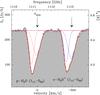 |
Fig. 1 Spectrum of the nucleus of NGC 4945 taken with Band 4b of Herschel-HIFI. Dotted lines indicate individual fit components and the solid line is the sum of these. The arrows indicate the systemic velocities for the H2O and H2O+ lines. The velocity scale refers to the H2O line, and is relative to a systemic velocity of V0 = 563 km s-1. |
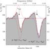 |
Fig. 2 As previous figure, for NGC 253, using V0 = 243 km s-1. |
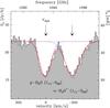 |
Fig. 3 As previous figure, for Arp 220, using V0 = 5434 km s-1. |
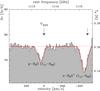 |
Fig. 4 As previous figure, for M 82c, using V0 = 203 km s-1. |
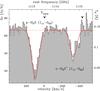 |
Fig. 5 As previous figure, for M 82NE, using V0 = 203 km s-1. |
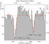 |
Fig. 6 As previous figure, for M 82SW, using V0 = 203 km s-1. |
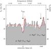 |
Fig. 7 As previous figure, for Cen A, V0 = 547 km s-1. |
3.1. Line profiles
Figures 1–7 present the calibrated 1113−1115 GHz spectra, both in Sν and TA units, on velocity and frequency axes. The H2O and H2O+ lines are detected in all five sources, and strong continuum is also seen. The appearance of the lines differs from source to source as discussed below. The reported continuum temperature is half the observed value because continuum radiation enters the receiver through both sidebands while the line is only in one sideband.
Toward NGC 4945, the H2O and H2O+ lines appear in absorption, the shape of which is well fitted with a double Gaussian. The derived parameters for the two lines are very similar to each other, and also similar to lines of HF observed with Herschel (Monje et al. 2014) and of HI observed with the VLA (Ott et al. 2001). The broad absorption component is centered close to the systemic velocity, while the narrower component is redshifted by ≈80 km s-1. As discussed by Monje et al. (2014), this appearance suggests an origin in a molecular gas ring that is possibly undergoing infall. Alternatively, redshifted absorption may result from non-circular gas motions, for instance in a barred potential.
The spectrum of NGC 253 shows a combination of emission and absorption for both lines, although the central velocities of H2O and H2O+ differ by 21–56 km s-1. Such P Cygni profiles are indicative of gas outflow, which is also seen in other species, perhaps most dramatically in OH with Herschel/PACS (Sturm et al. 2011). Other species such as HF (Monje et al. 2014) and HI (Koribalski et al. 1995) show absorption profiles with a similar shape as the H2O and H2O+ absorptions, but HI is without the corresponding emission feature.
The ultraluminous merger Arp 220 shows a single broad absorption in both species, which is so broad that they almost overlap. The two lines probably trace the same gas, although the H2O+ line is somewhat broader than that of H2O. The H2O+ profile may be influenced by a second absorption near −350 km s-1, which is of marginal significance. The centroid position of both lines suggests an origin in the western nucleus of the system (Aalto et al. 2007), which is suspected to harbor a supermassive black hole (Downes & Eckart 2007). Ground-based observations of H3O+ show a line at a similar velocity as H2O and H2O+, but with a smaller line width (Van der Tak et al. 2008).
The spectra toward the three positions in M 82 show narrow absorption in the H2O and H2O+ lines. The profiles toward M 82c show a possible weak secondary absorption feature that is redshifted from the main absorption by ≈50 km s-1. The H2O absorption toward M 82NE appears partially filled in by emission, unlike the H2O+ line and unlike the spectra at the other positions. Toward M 82SW, it is unclear whether the spectral excess between the H2O and H2O+ lines is due to line emission or a baseline artifact; we do not discuss it further.
The absorptions toward the “offset” NE and SW positions are actually deeper than toward the “central” M 82c position. Comparison with the high-resolution CO 1−0 map by Walter et al. (2002) shows that the NE and SW positions correspond to peaks in the CO distribution, while the central position is a local minimum in CO. We conclude that the H2O and H2O+ lines follow the distribution of molecular gas as traced by the CO 1−0 line.
The nearby radio galaxy Cen A appears to show inverse P Cygni profiles in the H2O and H2O+ lines, although the S/N ratio is limited. The derived parameters for the two lines are very similar, and the small velocity shift between the two lines is of marginal significance. The inverse P Cygni profile is a sign of gas infall, which in the case of Cen A may well be toward the central AGN. The H2O and H2O+ profiles are similar to those of CO and CI lines observed from the ground by Israel et al. (2014), except that the broad emission from the circumnuclear disk is not seen here.Following the nomenclature of Israel et al., the narrow H2O and H2O+ emission likely originates in the “extended thin disk” component of Cen A. The absorption components are also seen in CO , but they are not discussed by Israel et al.
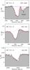 |
Fig. 8 Spectra of the OH+ 971 GHz line toward NGC 4945 (top), NGC 253 (middle), and Arp 220 (bottom). |
Figure 8 presents our spectra of the OH+ 971 GHz line toward NGC 4945, NGC 253, and Arp 220, where the line is clearly detected. The OH+ velocity profiles are similar to those of H2O and H2O+, with a double absorption toward NGC 4945 and a P Cygni-type line profile toward NGC 253. The spectrum of Arp 220 shows a single broad absorption as for the H2O and H2O+ lines, but the high signal-to-noise ratio reveals that this absorption has an asymmetric shape, which is indicative of an origin in a wind or absorption by the second nucleus.
The 971 GHz spectrum of NGC 4945 shows a second absorption feature right next to the OH+ line, which because of its mirrored shape probably originates from the image sideband. The most likely candidate is the CH3OH line at 959.4 GHz, since submm spectra of this galaxy show many lines from organic species (Wang et al. 2004). The NGC 4945 spectrum may also show a hint of an emission feature on the blueshifted shoulder of the OH+ line profile, which by itself is of marginal significance, but which may be real as it seems to have counterparts in H2O and possibly H2O+ (Fig. 1).
Measured line parameters.
3.2. Column densities
Based on the appearance of the lines, we have fitted Gaussian models to the profiles, and Table 2 presents the results. The asymmetric shape of the emission features suggests a geometry where some of the line emission is being absorbed by foreground material. To take this geometry into account, we simultaneously fit multiple Gaussians to the line profiles. The alternative of fitting separate Gaussians to the emission and absorption components would lead to lower line fluxes, but we consider this option less realistic.
To estimate the column densities of the absorption components, we assume negligible excitation (Tex<T10, where T10 = Eup/kB ≈ 50 K is the energy of the upper level above ground), so that only the molecular ground states are populated. For H2O, this assumption is justified by the multi-line radiative transfer analysis by L. Liu et al. (in prep.). For H2O and H2O+, we assume an ortho/para ratio of 3 as observed in Galactic interstellar clouds by Flagey et al. (2013) for H2O and Schilke et al. (2013) for H2O+. Under these assumptions, 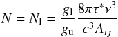 where gl and gu are the lower and upper state degeneracies, ν is the line frequency, and Aij is the Einstein A coefficient. These spectroscopic data are taken from the CDMS (Müller et al. 2005)2 and JPL (Pickett et al. 1998)3 catalogs; for OH+ and H2O+, we sum the contributions of the individual hyperfine components which are blended in our data. For a Gaussian profile, the velocity-integrated apparent optical depth is given by
 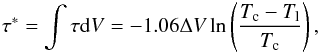 where the line and continuum antenna temperatures Tl and Tc and the FWHM line width ΔV are reported in Table 2. This expression assumes that the absorbing material covers the background continuum source homogeneously, and hence provides a lower limit to the actual line opacity. A patchy distribution with a higher opacity may be more realistic, as discussed by Weiß et al. (2010) for the case of M 82c.
To model the excitation of the emission components, we use the non-LTE radiative transfer program RADEX (Van der Tak et al. 2007)4 which includes collisional and radiative excitation, and treats optical depth effects with an escape probability formalism. For H2O we use state-of-the-art quantum-mechanically computed collision data with H2 from Daniel et al. (2011) as reported on the LAMDA database (Schöier et al. 2005)5. For OH+ we use collision rates with electrons from Van der Tak et al. (2013b) and use the rates with He from Gómez-Carrasco et al. (2014) to model inelastic collisions with H; collisions with H2 are mostly reactive in the case of OH+. For H2O+, detailed collisional calculations do not exist, so we approximate the collision rates of the radiatively allowed transitions as Q0 ∗ Sij, where Q0 is a characteristic downward rate coefficient and Sij is the normalized radiative line strength out of upper level i summed over all lower states, which enters the calculation of Aij from the microwave intensity. For the H2O+-H2 system, we adopt Q0 ~ 10-10 cm3 s-1 since H2O+ has a high dipole moment which should exhibit strong coupling to the H2 molecule.
Beam-averaged column densities and abundances.
We have run a grid of RADEX models covering kinetic temperatures from 10 to 100 K and H2 volume densities from 104 to 106 cm-3; for OH+, we assume n(H) = n(H2) and n(e)/n(H) = 10-4. These ranges should bracket the likely physical conditions in the nuclei of our sample galaxies (see Sect. 4). For all three species, we find Tex values from 3.4 K at low temperature and density to ≈9 K at high temperature and density. The optical depths of the lines scale linearly with the molecular column density up to N = 1014 cm-2, where τ = 0.4 is reached. We conclude from these calculations that under the likely conditions in the gas studied here, we may expect low excitation temperatures (5−10 K) for our studied species, which is indeed well below T10 as assumed above for the absorption components. A second conclusion is that for these lines, the optically thin assumption is only valid for column densities up to ~1014 cm-2.
As an alternative to collisions, radiative pumping may dominate the excitation of the emission components, as found for high-J lines of H2O in data from SPIRE (Yang et al. 2013), PACS (González-Alfonso et al. 2014), and HIFI (L. Liu et al., in prep.).For our 3 species, we model this case by adopting Tex = 100 K for all lines, which lowers our estimates of the total column density by factors of ≈15 relative to the values for Tex = 10 K. Further increasing Tex does not change the estimates much, as we approach the limit Tex≫T10.
3.3. Abundances
Table 3 lists our derived column densities, where we adopt Tex = 10 K for emission components, as found above as an average value between the cases of collisional and radiative excitation, and use the formula from Van der Tak et al. (2013b). The uncertainties on the column densities are factors of 5−10 for emission components, mainly through the uncertain Tex. The absorption column densities have small uncertainties, 10−15%, limited by calibration error, if the absorbers fill most of the HIFI beam, but the uncertainty is higher if the covering fraction is small and the absorption saturated. Uncertainties on column density ratios should be much smaller than for absolute column densities, because the various sources of error cancel out at least partially.
The column density values range over a factor of ~100 for the species that are detected in all sources: from 4 × 10¹² to 4.5 × 1014 cm-2 for H2O+, and from 1.8 × 10¹³ to 1.8 × 1015 cm-2 for H2O. The column density variation is smaller for OH+, which is only seen in three of our sources. Our H2O and H2O+ column densities for M 82c are 5−10× lower than those in Weiß et al. (2010) because we use the observed continuum instead of a model value. The column densities toward the M 82SW position are within 30% of those toward M 82c, while those toward M 82NE are ~2−4× higher, which follows the trend in the CO 1−0 emission map by Walter et al. (2002). In the cases where line emission is detected, the derived column densities are ~10−90% of the value estimated from the corresponding absorption feature, with an average value of 52%. The case of OH+ in NGC 253 follows this trend since the absorption feature is saturated so its column density is a lower limit. The fact that similar columns of gas (to a factor of 2) are probed in emission and absorption suggests that the nuclear region does not contribute much to the line emission, at least in the ground-state transitions.
Table 3 also presents column density ratios of H2O and OH+ over H2O+. The H2O/H2O+ ratios range from 1.4 to 5.6, which is at the low end of the distribution of H2O/H2O+ ratios for Galactic sources compiled by Wyrowski et al. (2010b). Studying lines of sight toward high-mass star-forming regions, these authors found H2O/H2O+ ratios of ~3 toward low-density gas (foreground clouds and outflow lobes) and higher ratios (~10) toward dense protostellar envelopes. Comparing our results with this Galactic study, our low observed H2O/H2O+ ratios suggest an origin of the emission and absorption features in diffuse gas clouds.
The right-hand column of Table 3 presents estimates of the H2O abundances toward our sources. These were obtained by dividing the N(H2O) values by estimates of N(H2) in similar-sized telescope beams. For NGC 4945, we adopt N(H2) = 1.0 × 1023 cm-2, based on 13CO and C18O observations at 230 GHz with the 15-m SEST telescope (Chou et al. 2007). For NGC 253, Weiß et al. (2008) estimate N(H2) = 1.5 × 1023 cm-2 based on APEX/LABOCA maps of 870 μm dust emission. For Arp 220, we use N(H2) = 1 × 1024 cm-2 as derived by Downes & Eckart (2007) for the extended disk/torus surrounding the western nucleus (cf. Aalto et al. 2009). For M 82c, we adopt N(H2) = 9 × 1022 cm-2 based on the discussion in Weiß et al. (2010). For Cen A, Israel et al. (2014) estimate N(H2) = 1.7 × 1022 cm-2 for the circumnuclear disk with a 20′′ diameter. The resulting abundances may be considered lower limits, as they compare the total amount of H2 to the fraction of gas in absorption (the foreground). However, the fact that we find similar column densities in emission and absorption suggests that this effect is small.
The H2O abundances in Table 3 range from 6.2 × 10⁻¹⁰ to 9.3 × 10⁻⁹, which is ~5–80× lower than typical values for Galactic diffuse clouds, where the H2O abundance is limited by photodissociation (Flagey et al. 2013). Our abundance values are in the normal range for cold dense Galactic gas clouds, where H2O is depleted on the surfaces of dust grains (Van Dishoeck et al. 2013), and somewhat below the usual values for warm dense gas (10-8–10-6: e.g., Emprechtinger et al. 2013). However, an origin of the H2O lines in dense clouds appears inconsistent with our observed H2O/H2O+ ratios, which are well below the value of ~10 for dense gas. One possibility may be that the H2O lines arise in dense clumps embedded in more diffuse gas where the OH+ and H2O+ lines originate, as suggested earlier to explain observed CO/CI ratios (e.g., Kramer et al. 2005). The similar shapes of the OH+ and H2O+ velocity profiles to those of both H2O and HI then indicate that the diffuse and dense gas phases are well mixed. We conclude that while the OH+ and H2O+ lines likely arise in diffuse gas clouds, the origin of the H2O lines is somewhat uncertain.
4. Discussion
To estimate the cosmic-ray ionization rates in our sample of galaxies from our H2O+ and OH+ observations, we assume steady-state ion-molecule chemistry (e.g., Hollenbach et al. 2012). Table 4 lists the relevant reactions and our adopted rates, which are taken from the UMIST database for astrochemistry (McElroy et al. 2013)6. In diffuse interstellar clouds, cosmic-ray ionization of H leads to H+, which charge transfers with O to form O+, which reacts with H2 to form OH+. The OH+ ion may recombine with a free electron (reaction 2) or react with H2 into H2O+ (reaction 1), which may itself recombine with an electron (reaction 4) or react with H2 into H3O+ (reaction 3), which recombines into H2O and other products.
As shown by Indriolo et al. (2012), the cosmic-ray ionization rate may be written in terms of observables as 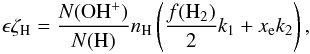 where the molecular hydrogen fraction f(H2), defined as
 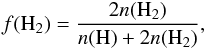 is related to the OH+/H2O+ ratio by
 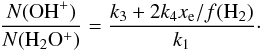 In these equations, ki is the rate of reaction i as listed in Table 4,and ϵ is the OH+ formation efficiency, which accounts for backward charge transfer from O+ to H and the neutralization of H+ on PAHs and dust grains (Neufeld et al. 2010). The only observational determination of this efficiency, based on OH+, H2O+ and H spectroscopy toward the W51 region (Indriolo et al. 2012), indicates ϵ ≈ 7%, which is in the range predicted by recent chemical models (Hollenbach et al. 2012). The reaction rates in Table 4 have been evaluated at an assumed typical temperature of T = 100 K, but our results are insensitive to this assumption as the reactions with H2 (k1 and k3) are independent of T and the recombination rates (k2 and k4) have a weak T-0.5 dependence (McElroy et al. 2013).
By the last equation, our observed OH+/H2O+ column density ratios of 1.6−3.1 (Table 3, Col. 6) indicate molecular fractions from f(H2) = 8% for the absorption component of NGC 253 to 20% for Arp 220.Our average OH+/H2O+ ratio of 2.5 corresponds to f(H2) = 11%, which is somewhat higher than the typical value of 4% for Galactic clouds (Indriolo et al. 2015). This result depends only on the column density ratio, so that any underestimates of the absolute column densities (e.g., due to filling factor assumptions) would cancel out. For the diffuse type of interstellar clouds where the OH+ and H2O+ lines thus likely originate, the electron abundance xe should equal the abundance of carbon since essentially all electrons come from photoionization of C. We adopt xe = 1.5 × 10⁻⁴ (Sofia et al. 2004) although values up to 2 × 10⁻⁴ may be possible (Sofia et al. 2011).
The final parameter needed to estimate the cosmic-ray ionization rate is the column density of atomic hydrogen. Although [HI] 21 cm observations exist for all our galaxies, high-resolution data in beams matching our HIFI observations only exist for M 82 (Yun et al. 1993) and Cen A (Van der Hulst et al. 1983). These data indicate N(H) values that are 3−5 times lower than the corresponding N(H2) numbers, suggesting that integrated over the line of sight, most gas is dense. On the other hand, the low f(H2) values derived above indicate that locally in the OH+- and H2O+-absorbing clouds, most gas is diffuse. The similarity of the OH+ and H2O+ line profiles to those of H2O as well as those of HI (Sect. 3.1) further indicates that the dense and diffuse gas phases are well mixed. Taken together, the data suggest a picture where the OH+-H2O+ absorbers are diffuse pockets or “bubbles” in a sea of dense gas.Assuming a typical gas density of nH = 35 cm-3 (Indriolo et al. 2015),the column densities in Table 3 indicate cosmic-ray ionization rates between 6 × 10-17 and 8 × 10-16 s-1, with an average value of 3.4 × 10⁻¹⁶ s-1. The uncertainty on these values is substantial (factors of 2−3), both through the absolute column densities (Table 3) and the model assumptions. For galaxies where OH+ or matched-beam HI data are unavailable, the uncertainty is even higher (factors of 3−5), as average OH+/H2O+ or H/H2 column density ratios must be assumed. These cases do not bias our results toward high or low ionization rates, so that our average value seems to be representative for our sample of sources.
Chemical network.
5. Conclusions
The cosmic-ray ionization rates derived in Sect. 4 are ~100× below estimates for molecular gas in AGN from excited-state H3O+ emission in the far-infrared (González-Alfonso et al. 2013), which themselves are in line with the high γ-ray fluxes, radio synchrotron luminosities, and supernova rates in such systems (e.g., Persic & Rephaeli 2012). Our ζH values are also ~10× below estimates for the Galactic center from H mid-infrared absorption (Goto et al. 2014), H3O+ submm emission (Van der Tak et al. 2008), and OH+ and H2O+ far-infrared absorption (Indriolo et al. 2015). They are, however, similar to values derived for the disk of our Galaxy from H absorption lines (Indriolo & McCall 2012), HCO+ submm emission (Van der Tak & van Dishoeck 2000), and OH+ and H2O+ absorption (Indriolo et al. 2015).
Together with the apparent low excitation state of the molecules (Sect. 3.2), these low inferred ζH values suggest that the low-J lines of OH+, H2O+, and H2O trace the extended gas in the disks of our galaxies, rather than the warm dense circumnuclear gas probed by their high-excitation lines. The gas probed by the low-J lines may either be physically distant from any nuclear activity, or it may be shielded from its radiation by large columns of dust, as also seen in the Spitzer mid-infrared spectra of obscured AGN (Lahuis et al. 2007). The observed (inverse) P Cygni profiles make the second option appear the most likely.
We conclude that the cosmic-ray ionization rate is not one constant that applies for a galaxy as a whole. Instead, ζH appears to vary by a factor of ~10 between the disk of a galaxy and its nucleus; variations of similar magnitude appear to exist between galaxies. These variations are in line with changes in chemical composition between the disks and the nuclei of galaxies (e.g., González-Alfonso et al. 2012) and also with the different ζH values found for the disk of our Galaxy and its nucleus (Van der Tak et al. 2006; Indriolo et al. 2015).
In the near future, ALMA and JWST will be instrumental to explore further differentiation between the various components of galaxies in terms of their physical and chemical conditions, including their ionization rates. In the longer term, the SPICA mission will extend the present work to systems at higher redshift, and characterize the interstellar media of galaxies out to the peak of cosmic star formation at z = 2.
Acknowledgments
The authors thank Russ Shipman (SRON) for help with data reduction, John Black (Onsala) and Fred Lahuis (SRON) for useful discussions, François Lique (Le Havre) for sending OH+-He collision data, and Paul van der Werf & Harold Linnartz (Leiden) for comments on the manuscript. This research has used the following databases: NED, SIMBAD, ADS, CDMS, JPL, and LAMDA. HIFI was designed and built by a consortium of institutes and university departments from across Europe, Canada and the US under the leadership of SRON Netherlands Institute for Space Research, Groningen, The Netherlands with major contributions from Germany, France and the US. Consortium members are: Canada: CSA, U.Waterloo; France: CESR, LAB, LERMA, IRAM; Germany: KOSMA, MPIfR, MPS; Ireland: NUI Maynooth; Italy: ASI, IFSI-INAF, Arcetri-INAF; Netherlands: SRON, TUD; Poland: CAMK, CBK; Spain: Observatorio Astronómico Nacional (IGN), Centro de Astrobiología (CSIC-INTA); Sweden: Chalmers University of Technology – MC2, RSS & GARD, Onsala Space Observatory, Swedish National Space Board, Stockholm University – Stockholm Observatory; Switzerland: ETH Zürich, FHNW; USA: Caltech, JPL, NHSC.
References
- Aalto, S., Spaans, M., Wiedner, M. C., & Hüttemeister, S. 2007, A&A, 464, 193 [NASA ADS] [CrossRef] [EDP Sciences] [Google Scholar]
- Aalto, S., Wilner, D., Spaans, M., et al. 2009, A&A, 493, 481 [NASA ADS] [CrossRef] [EDP Sciences] [Google Scholar]
- Aalto, S., Costagliola, F., van der Tak, F., & Meijerink, R. 2011, A&A, 527, A69 [NASA ADS] [CrossRef] [EDP Sciences] [Google Scholar]
- Benz, A. O., Bruderer, S., van Dishoeck, E. F., et al. 2010, A&A, 521, L35 [NASA ADS] [CrossRef] [EDP Sciences] [Google Scholar]
- Chou, R. C. Y., Peck, A. B., Lim, J., et al. 2007, ApJ, 670, 116 [NASA ADS] [CrossRef] [Google Scholar]
- Daniel, F., Dubernet, M.-L., & Grosjean, A. 2011, A&A, 536, A76 [NASA ADS] [CrossRef] [EDP Sciences] [Google Scholar]
- De Graauw, T., Helmich, F. P., Phillips, T. G., et al. 2010, A&A, 518, L6 [NASA ADS] [CrossRef] [EDP Sciences] [Google Scholar]
- Downes, D., & Eckart, A. 2007, A&A, 468, L57 [NASA ADS] [CrossRef] [EDP Sciences] [Google Scholar]
- Emprechtinger, M., Lis, D. C., Rolffs, R., et al. 2013, ApJ, 765, 61 [NASA ADS] [CrossRef] [Google Scholar]
- Flagey, N., Goldsmith, P. F., Lis, D. C., et al. 2013, ApJ, 762, 11 [NASA ADS] [CrossRef] [Google Scholar]
- Gómez-Carrasco, S., Godard, B., Lique, F., et al. 2014, ApJ, 794, 33 [NASA ADS] [CrossRef] [Google Scholar]
- González-Alfonso, E., Fischer, J., Graciá-Carpio, J., et al. 2012, A&A, 541, A4 [NASA ADS] [CrossRef] [EDP Sciences] [Google Scholar]
- González-Alfonso, E., Fischer, J., Bruderer, S., et al. 2013, A&A, 550, A25 [NASA ADS] [CrossRef] [EDP Sciences] [Google Scholar]
- González-Alfonso, E., Fischer, J., Aalto, S., & Falstad, N. 2014, A&A, 567, A91 [NASA ADS] [CrossRef] [EDP Sciences] [Google Scholar]
- Goto, M., Geballe, T. R., Indriolo, N., et al. 2014, ApJ, 786, 96 [NASA ADS] [CrossRef] [Google Scholar]
- Grenier, I. A., Black, J. H., & Strong, A. W. 2015, ARA&A, 53, 199 [NASA ADS] [CrossRef] [Google Scholar]
- Hollenbach, D., Kaufman, M. J., Neufeld, D., Wolfire, M., & Goicoechea, J. R. 2012, ApJ, 754, 105 [NASA ADS] [CrossRef] [Google Scholar]
- Indriolo, N., & McCall, B. J. 2012, ApJ, 745, 91 [NASA ADS] [CrossRef] [Google Scholar]
- Indriolo, N., Neufeld, D. A., Gerin, M., et al. 2012, ApJ, 758, 83 [NASA ADS] [CrossRef] [Google Scholar]
- Indriolo, N., Neufeld, D. A., Gerin, M., et al. 2015, ApJ, 800, 40 [NASA ADS] [CrossRef] [Google Scholar]
- Israel, F. P., Güsten, R., Meijerink, R., et al. 2014, A&A, 562, A96 [NASA ADS] [CrossRef] [EDP Sciences] [Google Scholar]
- Kennicutt, R. C., & Evans, N. J. 2012, ARA&A, 50, 531 [NASA ADS] [CrossRef] [Google Scholar]
- Koribalski, B., Whiteoak, J. B., & Houghton, S. 1995, PASA, 12, 20 [Google Scholar]
- Kramer, C., Mookerjea, B., Bayet, E., et al. 2005, A&A, 441, 961 [NASA ADS] [CrossRef] [EDP Sciences] [Google Scholar]
- Lahuis, F., Spoon, H. W. W., Tielens, A. G. G. M., et al. 2007, ApJ, 659, 296 [NASA ADS] [CrossRef] [Google Scholar]
- McElroy, D., Walsh, C., Markwick, A. J., et al. 2013, A&A, 550, A36 [NASA ADS] [CrossRef] [EDP Sciences] [Google Scholar]
- Monje, R. R., Lord, S., Falgarone, E., et al. 2014, ApJ, 785, 22 [NASA ADS] [CrossRef] [Google Scholar]
- Müller, H. S. P., Schlöder, F., Stutzki, J., & Winnewisser, G. 2005, J. Mol. Struct., 742, 215 [NASA ADS] [CrossRef] [Google Scholar]
- Neufeld, D. A., Goicoechea, J. R., Sonnentrucker, P., et al. 2010, A&A, 521, L10 [NASA ADS] [CrossRef] [EDP Sciences] [Google Scholar]
- Oka, T., Geballe, T. R., Goto, M., Usuda, T., & McCall, B. J. 2005, ApJ, 632, 882 [NASA ADS] [CrossRef] [Google Scholar]
- Ott, M., Whiteoak, J. B., Henkel, C., & Wielebinski, R. 2001, A&A, 372, 463 [NASA ADS] [CrossRef] [EDP Sciences] [Google Scholar]
- Ott, S. 2010, in Astronomical Data Analysis Software and Systems XIX, eds. Y. Mizumoto, K.-I. Morita, & M. Ohishi, ASP Conf. Ser., 434, 139 [Google Scholar]
- Papadopoulos, P. P. 2010, ApJ, 720, 226 [NASA ADS] [CrossRef] [Google Scholar]
- Persic, M., & Rephaeli, Y. 2012, J. Phys. Conf. Ser., 355, 012038 [NASA ADS] [CrossRef] [Google Scholar]
- Pickett, H. M., Poynter, R. L., Cohen, E. A., et al. 1998, J. Quant. Spectr. Rad. Transf., 60, 883 [NASA ADS] [CrossRef] [Google Scholar]
- Pilbratt, G. L., Riedinger, J. R., Passvogel, T., et al. 2010, A&A, 518, L1 [CrossRef] [EDP Sciences] [Google Scholar]
- Porras, A. J., Federman, S. R., Welty, D. E., & Ritchey, A. M. 2014, ApJ, 781, L8 [NASA ADS] [CrossRef] [Google Scholar]
- Roelfsema, P. R., Helmich, F. P., Teyssier, D., et al. 2012, A&A, 537, A17 [NASA ADS] [CrossRef] [EDP Sciences] [Google Scholar]
- Schilke, P., Lis, D. C., Bergin, E. A., Higgins, R., & Comito, C. 2013, J. Phys. Chem. A, 117, 9766 [CrossRef] [PubMed] [Google Scholar]
- Schöier, F. L., van der Tak, F. F. S., van Dishoeck, E. F., & Black, J. H. 2005, A&A, 432, 369 [NASA ADS] [CrossRef] [EDP Sciences] [Google Scholar]
- Sofia, U. J., Lauroesch, J. T., Meyer, D. M., & Cartledge, S. I. B. 2004, ApJ, 605, 272 [NASA ADS] [CrossRef] [Google Scholar]
- Sofia, U. J., Parvathi, V. S., Babu, B. R. S., & Murthy, J. 2011, AJ, 141, 22 [NASA ADS] [CrossRef] [EDP Sciences] [Google Scholar]
- Sturm, E., González-Alfonso, E., Veilleux, S., et al. 2011, ApJ, 733, L16 [NASA ADS] [CrossRef] [Google Scholar]
- Van der Hulst, J. M., Golisch, W. F., & Haschick, A. D. 1983, ApJ, 264, L37 [NASA ADS] [CrossRef] [Google Scholar]
- Van der Tak, F. F. S., & van Dishoeck, E. F. 2000, A&A, 358, L79 [NASA ADS] [Google Scholar]
- Van der Tak, F. F. S., Belloche, A., Schilke, P., et al. 2006, A&A, 454, L99 [NASA ADS] [CrossRef] [EDP Sciences] [Google Scholar]
- Van der Tak, F. F. S., Black, J. H., Schöier, F. L., Jansen, D. J., & van Dishoeck, E. F. 2007, A&A, 468, 627 [NASA ADS] [CrossRef] [EDP Sciences] [Google Scholar]
- Van der Tak, F. F. S., Aalto, S., & Meijerink, R. 2008, A&A, 477, L5 [NASA ADS] [CrossRef] [EDP Sciences] [Google Scholar]
- Van der Tak, F. F. S., Chavarría, L., Herpin, F., et al. 2013a, A&A, 554, A83 [NASA ADS] [CrossRef] [EDP Sciences] [Google Scholar]
- Van der Tak, F. F. S., Nagy, Z., Ossenkopf, V., et al. 2013b, A&A, 560, A95 [NASA ADS] [CrossRef] [EDP Sciences] [Google Scholar]
- Van Dishoeck, E. F., Herbst, E., & Neufeld, D. A. 2013, Chem. Rev., 113, 9043 [NASA ADS] [CrossRef] [PubMed] [Google Scholar]
- Walter, F., Weiss, A., & Scoville, N. 2002, ApJ, 580, L21 [NASA ADS] [CrossRef] [Google Scholar]
- Wang, M., Henkel, C., Chin, Y.-N., et al. 2004, A&A, 422, 883 [NASA ADS] [CrossRef] [EDP Sciences] [Google Scholar]
- Weiß, A., Kovács, A., Güsten, R., et al. 2008, A&A, 490, 77 [NASA ADS] [CrossRef] [EDP Sciences] [Google Scholar]
- Weiß, A., Requena-Torres, M. A., Güsten, R., et al. 2010, A&A, 521, L1 [NASA ADS] [CrossRef] [EDP Sciences] [Google Scholar]
- Wyrowski, F., Menten, K. M., Güsten, R., & Belloche, A. 2010a, A&A, 518, A26 [NASA ADS] [CrossRef] [EDP Sciences] [Google Scholar]
- Wyrowski, F., van der Tak, F., Herpin, F., et al. 2010b, A&A, 521, L34 [NASA ADS] [CrossRef] [EDP Sciences] [Google Scholar]
- Yang, C., Gao, Y., Omont, A., et al. 2013, ApJ, 771, L24 [NASA ADS] [CrossRef] [Google Scholar]
- Yun, M. S., Ho, P. T. P., & Lo, K. Y. 1993, ApJ, 411, L17 [NASA ADS] [CrossRef] [Google Scholar]
- Zhao, D., Galazutdinov, G. A., Linnartz, H., & Krełowski, J. 2015, ApJ, 805, L12 [NASA ADS] [CrossRef] [Google Scholar]
All Tables
All Figures
|
Fig. 1 Spectrum of the nucleus of NGC 4945 taken with Band 4b of Herschel-HIFI. Dotted lines indicate individual fit components and the solid line is the sum of these. The arrows indicate the systemic velocities for the H2O and H2O+ lines. The velocity scale refers to the H2O line, and is relative to a systemic velocity of V0 = 563 km s-1. |
| In the text | |
|
Fig. 2 As previous figure, for NGC 253, using V0 = 243 km s-1. |
| In the text | |
|
Fig. 3 As previous figure, for Arp 220, using V0 = 5434 km s-1. |
| In the text | |
|
Fig. 4 As previous figure, for M 82c, using V0 = 203 km s-1. |
| In the text | |
|
Fig. 5 As previous figure, for M 82NE, using V0 = 203 km s-1. |
| In the text | |
|
Fig. 6 As previous figure, for M 82SW, using V0 = 203 km s-1. |
| In the text | |
|
Fig. 7 As previous figure, for Cen A, V0 = 547 km s-1. |
| In the text | |
|
Fig. 8 Spectra of the OH+ 971 GHz line toward NGC 4945 (top), NGC 253 (middle), and Arp 220 (bottom). |
| In the text | |
Current usage metrics show cumulative count of Article Views (full-text article views including HTML views, PDF and ePub downloads, according to the available data) and Abstracts Views on Vision4Press platform.
Data correspond to usage on the plateform after 2015. The current usage metrics is available 48-96 hours after online publication and is updated daily on week days.
Initial download of the metrics may take a while.