| Issue |
A&A
Volume 592, August 2016
|
|
|---|---|---|
| Article Number | L8 | |
| Number of page(s) | 4 | |
| Section | Letters | |
| DOI | https://doi.org/10.1051/0004-6361/201628769 | |
| Published online | 08 August 2016 | |
O VI 1032 Å intensity and Doppler shift oscillations above a coronal hole: Magnetosonic waves or quasi-periodic upflows?
1 Istituto Nazionale di Astrofisica,
Osservatorio Astrofisico di Torino, Strada Osservatorio 20, 10025 Pino
Torinese, Italy
e-mail: mancuso@oato.inaf.it
2 Harvard-Smithsonian Center for
Astrophysics, 60 Garden Street, MS 50, Cambridge, MA
02138,
USA
3 Dipartimento di Fisica, Università
degli studi di Torino, Via P.
Giuria 1, 10125
Torino,
Italy
Received:
22
April
2016
Accepted:
18
July
2016
On 1996 December 19, the Ultraviolet Coronagraph Spectrometer (UVCS) on board the Solar and Heliospheric Observatory (SOHO) conducted a special high-cadence sit-and-stare observation in the O vi 1032 Å spectral line above a polar coronal hole at a heliocentric distance of 1.38 R⊙. The ~ 9-h dataset was analyzed by applying advanced spectral techniques to investigate the possible presence of propagating waves. Highly significant oscillations in O vi intensity (P = 19.5 min) and Doppler shift (P = 7.2 min) were detected over two different portions of the UVCS entrance slit. A cross-correlation analysis between the O vi intensity and Doppler shift fluctuations shows that the most powerful oscillations were in phase or anti-phase over the same portions of the slit, thus providing a possible signature of propagating magnetosonic waves. The episodic nature of the observed oscillations and the large amplitudes of the Doppler shift fluctuations detected in our observations, if not attributable to line-of-sight effects or inefficient damping, may indicate that the observed fluctuations were produced by quasi-periodic upflows.
Key words: Sun: corona / Sun: UV radiation / Sun: oscillations / magnetohydrodynamics (MHD)
© ESO, 2016
1. Introduction
Remote sensing observations obtained using imaging and spectroscopic techniques from instruments on board different spacecraft suggest that both Alfvén waves and slow magnetosonic waves are present in polar coronal holes (e.g., Banerjee et al. 2011). The observation of magnetohydrodynamic (MHD) waves in the solar corona provides valuable insights into unsolved problems in coronal physics since these waves may contribute to the heating of the solar corona and the acceleration of the fast component of the solar wind (see Nakariakov et al. 2016, for a recent review). Bright quasi-radial ray-like structures, the so-called coronal plumes, are usually seen in the off-limb part of polar coronal holes originating in photospheric unipolar magnetic flux concentrations. Being regions of lower Alfvén speed stretched along the radial magnetic field, coronal plumes represent natural waveguides for different MHD waves. The first clear detection of MHD waves in polar coronal holes was obtained by analyzing polarized brightness (pB) data from the white-light channel of the Ultraviolet Coronagraph Spectrometer (UVCS; Kohl et al. 1995) on board the Solar and Heliospheric Observatory (SOHO). The density fluctuations of period P ~ 9 min observed by Ofman et al. (1997) at the height of 1.9 R⊙ were attributed to the propagation of slow magnetosonic waves in polar plumes. A number of studies followed reporting such oscillations in plumes and interplumes by using spectroscopic data obtained with EUV instruments. Although most of the early detections of fluctuations in coronal holes were interpreted in terms of propagating slow magnetosonic waves, recent spectroscopic observations have challenged this interpretation by posing a more complex picture that implies recurrent jet-like mass motions. Quasi-periodic vertical upflows can in fact produce oscillatory perturbations in intensity as well as in Doppler velocity, line-widths, and red-blue asymmetries. A thorough discussion on the problematics of distinguishing between propagating waves and quasi-periodic upflows is given in the review by De Moortel & Nakariakov (2012). In this Letter, we present the spectral analysis of a special high-cadence observation in the O vi 1032 Å spectral line obtained on 1996 December 19 at a heliocentric distance of 1.38 R⊙ above a polar coronal hole and provide evidence for the presence of highly significant coronal oscillations in both intensity and Doppler shift. This detection was made possible by the availability of a new accurate calibration of the UVCS data and the application of advanced spectral analysis techniques. These observations have the potential to shed new light on the possible presence of large-amplitude magnetosonic waves in the middle corona.
2. Observations and data reduction
The observations analyzed in this work were obtained on 1996 December 19 with the UV spectral channel of the UVCS telescope that is optimized for the study of the O vi doublet 1031.91 Å and 1037.61 Å. The data were collected during a special high-cadence sit-and-stare observation, with the entrance slit centered over the north pole at a heliocentric distance of 1.38 R⊙ (see Fig. 1). The observations began at 19:10 UT and ended on the next day at 4:54 UT with a cadence of about 66 s for a total of 529 exposures. Owing to the limited telemetry rate available to UVCS, the spectral window for this observation was confined to a 4.76 Å band centered on the O vi 1032 Å line in order to achieve high spectral and spatial resolution and high image cadence. The 0.3 mm slit (corresponding to a spatial width of 84′′ or 1.08 Å) extended over about 66.5° in position angle from −896.0′′ to + 889.0′′ with data binned to 7′′ (1 px) along the 1785′′ slit length, thus providing 255 spatial bins. Spectral binning was 2 px, yielding a spectral resolution of 0.1983 Å with 24 bins in the dispersion direction. The latest UVCS Data Display and Analysis Software, Version 5.1 (DAS51) was used to remove image distortion and to calibrate the data in wavelength and intensity. A few hours before the beginning at 19:10 UT of the UVCS sit-and-stare observation, a wide (>180°) coronal mass ejections (CME) was reported in the online CME Catalog1 propagating on the west limb with an average speed of 142 km s-1 and an extrapolated onset at 15:33 UT. The eruption was probably related to a C 2.3 class flare detected by the GOES instrument on the same day above AR NOAA 8005 (located at coordinates S14 W09) with onset at 15:38 UT and peak at 16:10 UT. The first fifty exposures of the UVCS observations were excluded from the following analysis since the spectra were found to be still affected by the propagation of the CME described above.
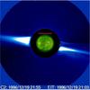 |
Fig. 1 Composite LASCO C2 and EIT Fe xii 195 Å image from 1996 December 19. The solid red line indicates the position of the UVCS slit at the time of the observation. |
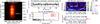 |
Fig. 2 a): O vi 1032 Å spectral line averaged over the whole observation. White dotted lines delineate the edges of the 182′′ portion of the UVCS slit (region A) analyzed here. b) Detrended O vi relative intensity variation over region A. c) LSP computed from the above time series. d) Wavelet power spectrum. The white grid indicates the region in which estimates of oscillation period become unreliable. e) Global wavelet power spectrum. Peaks above the 99% confidence level curve are statistically significant. f) Scale-average wavelet power in units of normalized variance. |
 |
Fig. 3 Same as Fig. 2 but for the detrended O vi Doppler shift variation time series integrated across a 259′′ region along the slit (region B). |
3. Analysis and results
Starting from 20:04 UT, a non-linear least-squares fit to a Gaussian plus a constant background was performed for all possible spatial binning intervals (>10 px to obtain a high signal-to-noise ratio) along the slit to yield the O vi 1032 Å Doppler shift and intensity at each exposure. Unfortunately, although the spectral resolution of this particular set of observations was high enough to determine Doppler shifts, the data were acquired with a slit width that was too large to allow us to disentangle the instrumental broadening from the intrinsic line width. To determine possible periodicities and ascertain their significance, we applied the Lomb-Scargle periodogram (LSP; Scargle 1982) technique, which allows reliable estimates of the level of significance of any detected periodic signal. The LSP was computed on the detrended time series of the two parameters (a second-order polynomial was subtracted prior to period search). A highly significant oscillation (P = 19.5 min) above the 99.99% confidence level (c.l.) (Fig. 2c) was detected in intensity across a 182′′ region from –336′′ to –154′′ along the slit (region A; Fig. 2a) with a relative rms amplitude of 9.6%. A highly significant oscillation (P = 7.2 min; >99.99% c.l.) was also detected in Doppler velocity across a 259′′ region from 63′′ to 322′′ along the slit (region B; Fig. 3a) with a rms amplitude of 11.8 km s-1. Stray light in UVCS observations at low heights could wash out the O vi signal in both intensity and velocity, thus causing a possible underestimation of the derived amplitudes. We verified that the N v 1242 Å line (including stray light) in synoptic observations taken on the next day at about the same height and position angle was at least 200 times fainter than the O vi line in the data we analyzed. Since the disk brightness of O vi is ~8 times larger than N v, the upper limit to the stray light is estimated as ~4%. Although the LSP technique is very successful in detecting sinusoidal periodic data, the observed fluctuations may somehow deviate from sinusoidal variation, thus leading to false detections. In fact, although wave fields are commonly described using the plane wave basis, wave-related motions or density enhancements can have a much more complex character. An alternative approach for time series analysis of non-stationary, noisy data that does not rely exclusively on sinusoidal bases is singular spectrum analysis (SSA; Broomhead & King 1986; Vautard et al. 1992), which decomposes a time series into a number of data-adaptive, non-sinusoidal components with simpler structures (see, e.g., Mancuso & Raymond 2015; Taricco et al. 2015). The SSA analysis confirmed the LSP results, revealing that the intensity time variation in region A is characterized by a component with a period of 19.5 min, which accounts for 10.6% of the total variance. A Monte Carlo test applied on the SSA spectrum demonstrated that this oscillation is significant at the 99.99% c.l. The SSA also confirmed the detection of the Doppler shift oscillation with period P = 7.2 min at the 99.9% c.l. (9.6% of total variance). The periods of the disturbances were further investigated using wavelet analysis (Torrence & Compo 1998). The wavelet methods allow the identification of periodic components in a time series and their variation in time by decomposing the series using scaled and translated versions of a wavelet basis function. The periodic signals detected in the Morlet wavelet spectra are visible in both cases as bright spots (the colored scale corresponds to the magnitude of the power) stretching along the time axis (Figs. 2d and 3d). Although several peaks are visible in the global wavelet spectrum (GWS) (Figs. 2e and 3e), which represents the average of the wavelet power over time at each oscillation period, the only fluctuations that have enough power (>99% c.l.) correspond to the ones already shown with the previous techniques. A plot of the average variance of the wavelet power of the detrended O vi relative intensity variation time series in a 3 min band around 19.5 min (Fig. 2f) shows that the periodic density fluctuations detected with this period exhibit a persistent behavior pattern during the observation with a coherence time of ≳ one hour (that is, about three to four oscillations). The Doppler shift fluctuations around 7 min (Fig. 3f) are, however, more episodic.
4. Discussion
The coronal O vi 1032 Å line is formed by both collisional excitation (followed by spontaneous radiative de-excitation) and resonant scattering of chromospheric radiation with the intensity of the collisional component scaling as  and the resonantly scattered component as ne. The O vi 1032 Å emission in this particular observation was due in about equal measure to resonant scattering and collisional excitation (see Noci et al. 1987 for details). Within the framework of the wave interpretation, the highly significant intensity oscillations (P = 19.5 min) detected in region A of the UVCS slit are compatible with the propagation of magnetosonic waves perturbing the density along the coronal structures over which they propagated. The rms amplitude (~10%) of the intensity variations detected in region A is in the lower range of the EUV brightness oscillations (P ~ 10−15 min) with relative amplitudes of 10−20% detected in plumes by DeForest & Gurman (1998) and interpreted as propagating slow magnetosonic waves by Ofman et al. (1999). In principle, the highly significant Doppler shift oscillations (P = 7.2 min) detected in region B could be alternatively attributed to transverse (or Alfvén) waves propagating substantially perpendicular to the line of sight (LOS); however, because they are incompressible, they would yield no periodic or correlated radiance signature. On the other hand, the signature of compressive waves may also be seen in Doppler velocity, as a result of plasma motions, when they have a significant component directed towards the observer. By applying the LSP to the intensity time series in region B, we find a dominant period of P = 7.4 min (below the 95% c.l.) with a rms amplitude of 8.5%, suggesting a common mechanism for the intensity and Doppler shift fluctuations detected in region B. Vice versa, by applying the LSP to the Doppler shift time series in region A, we find a dominant period of P = 14.0 min with a rms amplitude of 13.7 km s-1. This result (below the 95% c.l. and thus unreliable per se) does not match in periodicity the intensity oscillations observed in region A, maybe suggesting a different independent mechanism for their production (perhaps transverse or Alfvén waves?) as in Gupta et al. (2010) who detected accelerated propagating fluctuations in EUV intensity and Doppler shift with periods of 15−20 min in a coronal hole and interpreted them as likely due to Alfvénic or fast magnetoacoustic waves in the interplume region and slow magnetosonic waves in the plume region. We further note that the various possible interpretations are certainly limited by the unknown inclination angles that polar plumes present at higher heliocentric distances relative to the LOS. Polar plumes are actually seen to diverge super-radially and, during solar minimum conditions, they can be strongly inclined with respect to the plane of the sky, especially at higher heliocentric distances, because their roots can reach an extension down to 60° in solar latitude. The reason why the O vi Doppler shift oscillations were found to be dominant in region B or that the intensity oscillations in region A did not show a clear counterpart in Doppler shift could depend on the different inclination of the plume structures that support those waves with respect to the LOS: for nearly perpendicular plumes, we would preferentially detect intensity oscillations (as in region A); for highly tilted plumes, we would also observe Doppler shift oscillations (as in region B). This geometrical effect could tentatively explain why the amplitudes of the highly significant Doppler shifts detected in this work (~12 km s-1) are larger than those usually detected at lower heights (≲ 6 km s-1) (e.g., Gupta et al. 2012). Indeed, the amplitudes of the Doppler shift oscillations we detected in this particular set of observations seem quite large, even considering the expected decrease in amplitude at higher heliocentric distances due to dissipation mechanisms such as compressive viscosity and electron thermal conduction. Independently from their statistical significance over the 9-h observation, if the detected fluctuations were indeed episodic, as seen by the wavelet analysis, we expect at least to observe correlated or anti-correlated behavior over intervals of the time series that displayed maximum power in the wavelet spectrum. In particular, the phase at which an outward propagating magnetosonic wave would produce a blueshift of the line profile should coincide with a density (i.e., intensity) enhancement because of the in-phase behavior of velocity and density perturbations (e.g., Wang et al. 2009; Verwichte et al. 2010). A cross-correlation analysis between the O vi intensity and Doppler shift time series (Fig. 4) was thus performed over intervals of the time series that displayed maximum power in the wavelet spectrum for both regions A and B (a 5-point and 3-point moving average was applied, respectively, to the two time series to reduce the noise before cross-correlation). The cross-correlation function (CCF) as a function of time-lag revealed that the two oscillations were in phase over a time interval around 0 UT (Fig. 4) in region A and in anti-phase otherwise (the absolute value of the correlation at zero lag is always above the c.l.). In particular, if the two in-phase and anti-phase oscillations observed in region A came from the same coronal structure, this would imply propagation in one direction (upward or downward) at first (interval Δt1), but in the opposite direction later on (interval Δt2). Otherwise, if we assume that both oscillations were propagating along the same upward or downward direction, the two oscillations must have belonged to structures with different inclinations relative to the plane of sky. The wavelet analysis has indicated that some mechanism was driving the oscillations intermittently producing short bursts with coherence times of a few oscillations. McIntosh et al. (2010) analyzed high-cadence STEREO observations of brightness fluctuations in plumes and interpreted them in terms of quasi-periodically (P ~ 5−20 min) recurrent upflows with an apparent brightness enhancement of ~5% above that of the plumes they travel on. The large amplitude of the highly significant Doppler shift oscillations found in region B with respect to the values obtained at lower heights by EUV instruments, if not due to the enhanced inclination of the plume structures over which the waves propagate, might indicate that the damping mechanisms are actually not as effective as models predict or that the observed O vi fluctuations were not produced by magnetosonic waves but by quasi-periodic upflows. In fact, outflow velocities of ~50 km s-1 at 1.4 R⊙ (Gabriel et al. 2003; 2005) and inclinations of the plume structures of, e.g., 10−20°, would imply Doppler shifts of 9−17 km s-1, roughly corresponding to the span (trough to crest) of the periodic Doppler shifts observed in our time series. The key to discriminating between the two scenarios (waves versus flows) relies, however, on an accurate investigation of the temporal behavior of the observed line widths and line asymmetries (see, e.g., De Pontieu & McIntosh 2010) that unfortunately is not possible with the data analyzed in this work. Finally, in order to understand whether the two regions (A and B) in which we detected significant oscillations correspond to dense plume structures, we retrieved the white-light polarization brightness (pB) data taken by the MLSO Mk3 coronameter for the same day averaged over four hours starting from 17:42 UT (Fig. 5).
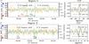 |
Fig. 4 Left panels: O vi 1032 Å relative intensity and Doppler shift variations over region A (top) and B (bottom). The time series have been denoised, respectively, with a 5-point and 3-point moving average. Vertical lines delineate the time interval over which the CCF (right panels) was calculated, roughly corresponding to the maximum power in the respective wavelet spectra. The red dotted lines are the c.l. |
The pB data were smoothed by using the IDL routine filter_image.pro that convolves all pixels in an image with a Gaussian kernel (an elliptical beam with FWHM = 5 × 20 px was used in this case). Clear plume structures are observed in both regions among the interplume material at about the same height as the UVCS entrance slit. However, the plumes are much thinner than the two portions of the UVCS slit corresponding to regions A and B so that the observed oscillations, if due to waves, were probably related to several plumes.
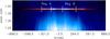 |
Fig. 5 Blue-scale image of a filtered average of white-light MLSO Mk3 observations taken on 1996 December 19. The average O vi 1032 Å line intensity distribution along the UVCS slit is superimposed. |
5. Conclusions
We analyzed a special high-cadence sit-and-stare UVCS observation in the O vi 1032 Å spectral line made on 1996 December 19 with the entrance slit placed at 1.38 R⊙ above a polar coronal hole. Spectral analysis of the ~9-h observation revealed two distinct regions along the UVCS slit with highly significant O vi intensity (P = 19.5 min) and Doppler shift (P = 7.2 min) oscillations and relative amplitudes of, respectively, ~10% and ~12 km s-1. A cross-correlation analysis between the O vi intensity and Doppler shift variations over intervals of the time series that displayed maximum power in the wavelet spectrum indicates that the most powerful fluctuations were in phase or anti-phase over the same portions of the slit, as expected in the case of propagating magnetosonic waves. The episodic nature of the observed oscillations and the large amplitudes of the Doppler shift fluctuations detected in our observations, if not attributable to LOS effects or inefficient damping, may be also interpreted in terms of quasi-periodic upflows. We note, however, that these two scenarios (waves versus upflows) are difficult to differentiate on the basis of the observations analyzed in this work and that both interpretations are limited by the unknown inclination angles that polar plumes present at higher heliocentric distances.
Acknowledgments
We are grateful to the anonymous referee for the suggestions that led to a substantial improvement of the manuscript. The UVCS is the result of a collaborative effort between NASA and ASI, with a Swiss participation. Mk3 data are courtesy of the MLSO, operated by the HAO, as part of the NCAR, supported by the National Science Foundation.
References
- Banerjee, D., Gupta, G. R., & Teriaca, L. 2011, Space Sci. Rev., 158, 267 [NASA ADS] [CrossRef] [Google Scholar]
- Broomhead, D. S., & King, G. P. 1986, Physica D: Nonlin. Phenom., 20, 217 [CrossRef] [Google Scholar]
- DeForest, C. E., & Gurman, J. B. 1998, ApJ, 501, L217 [NASA ADS] [CrossRef] [Google Scholar]
- De Moortel, I., & Nakariakov, V. M. 2012, Phil. Trans. Roy. Soc. London, 370, 3193 [Google Scholar]
- De Pontieu, B., & McIntosh, S. W. 2010, ApJ, 722, 1013 [NASA ADS] [CrossRef] [Google Scholar]
- Gabriel, A. H., Bely-Dubau, F., & Lemaire, P. 2003, ApJ, 589, 623 [NASA ADS] [CrossRef] [Google Scholar]
- Gabriel, A. H., Abbo, L., Bely-Dubau, F., et al. 2005, ApJ, 635, L185 [NASA ADS] [CrossRef] [Google Scholar]
- Gupta, G. R., Banerjee, D., Teriaca, et al. 2010, ApJ, 718, 11 [NASA ADS] [CrossRef] [Google Scholar]
- Gupta, G. R., Teriaca, L., Marsch, D., et al. 2012, A&A, 546, A93 [NASA ADS] [CrossRef] [EDP Sciences] [Google Scholar]
- Kohl, J. L., Esser, R., Gardner, L. D., et al. 1995, Sol. Phys., 162, 313 [NASA ADS] [CrossRef] [Google Scholar]
- Mancuso, S., & Raymond, J. C. 2015, A&A, 573, A33 [NASA ADS] [CrossRef] [EDP Sciences] [Google Scholar]
- McIntosh, S. W., Innes, D. E., de Pontieu, B., & Leamon, R. J. 2010, A&A, 510, L2 [NASA ADS] [CrossRef] [EDP Sciences] [Google Scholar]
- Nakariakov, V. M., Pilipenko, V., Heilig, B., et al. 2016, Space Sci. Rev., 200, 75 [NASA ADS] [CrossRef] [Google Scholar]
- Noci, G., Kohl, J. L., & Withbroe, G. L. 1987, ApJ, 315, 706 [NASA ADS] [CrossRef] [Google Scholar]
- Ofman, L., Romoli, M., Poletto, G., Noci, G., & Kohl, J. L. 1997, ApJ, 491, L111 [NASA ADS] [CrossRef] [Google Scholar]
- Ofman, L., Nakariakov, V. M., & DeForest, C. E. 1999, ApJ, 514, 441 [NASA ADS] [CrossRef] [Google Scholar]
- Scargle, J. D. 1982, ApJ, 263, 835 [NASA ADS] [CrossRef] [Google Scholar]
- Taricco, C., Mancuso, S., Ljungqvist, F. C., Alessio, S., & Ghil, M. 2015, Climate Dynamics, 45, 83 [Google Scholar]
- Torrence, C., & Compo, G. P. 1998, Bull. Amer. Meteor. Soc., 79, 61 [CrossRef] [Google Scholar]
- Vautard, R., Yiou, P., & Ghil, M. 1992, Physica D: Nonlin. Phenom., 58, 95 [Google Scholar]
- Verwichte, E., Marsh, M., Foullon, C., et al. 2010, ApJ, 724, L194 [NASA ADS] [CrossRef] [Google Scholar]
- Wang, T. J., Ofman, L., Davila, J. M., & Mariska, J. T. 2009, A&A, 503, L25 [NASA ADS] [CrossRef] [EDP Sciences] [Google Scholar]
All Figures
|
Fig. 1 Composite LASCO C2 and EIT Fe xii 195 Å image from 1996 December 19. The solid red line indicates the position of the UVCS slit at the time of the observation. |
| In the text | |
|
Fig. 2 a): O vi 1032 Å spectral line averaged over the whole observation. White dotted lines delineate the edges of the 182′′ portion of the UVCS slit (region A) analyzed here. b) Detrended O vi relative intensity variation over region A. c) LSP computed from the above time series. d) Wavelet power spectrum. The white grid indicates the region in which estimates of oscillation period become unreliable. e) Global wavelet power spectrum. Peaks above the 99% confidence level curve are statistically significant. f) Scale-average wavelet power in units of normalized variance. |
| In the text | |
|
Fig. 3 Same as Fig. 2 but for the detrended O vi Doppler shift variation time series integrated across a 259′′ region along the slit (region B). |
| In the text | |
|
Fig. 4 Left panels: O vi 1032 Å relative intensity and Doppler shift variations over region A (top) and B (bottom). The time series have been denoised, respectively, with a 5-point and 3-point moving average. Vertical lines delineate the time interval over which the CCF (right panels) was calculated, roughly corresponding to the maximum power in the respective wavelet spectra. The red dotted lines are the c.l. |
| In the text | |
|
Fig. 5 Blue-scale image of a filtered average of white-light MLSO Mk3 observations taken on 1996 December 19. The average O vi 1032 Å line intensity distribution along the UVCS slit is superimposed. |
| In the text | |
Current usage metrics show cumulative count of Article Views (full-text article views including HTML views, PDF and ePub downloads, according to the available data) and Abstracts Views on Vision4Press platform.
Data correspond to usage on the plateform after 2015. The current usage metrics is available 48-96 hours after online publication and is updated daily on week days.
Initial download of the metrics may take a while.