© ESO, 2016

1. Introduction

The Yarkovsky-O’Keefe-Radzievskii-Paddack (YORP) effect is the torque experienced by an asteroid owing to its asymmetric emission of incident light pressure radiation by its surface (Rubincam 2000; Bottke et al. 2006; Vokrouhlický et al. 2015). It is useful to divide the YORP torque into two components: normal YORP (NYORP) is created by light pressure forces that are normal to the large-scale surface of the asteroid, which do not cancel each other’s torques because of large-scale asymmetries in the asteroid’s shape (Rubincam 2000). Tangential YORP (TYORP) is created by light pressure forces tangential to the large-scale surface, which are non-zero because stones lying on the surface emit different amounts of infrared light eastward and westward (Golubov & Krugly 2012). Any asteroid is, to some extent, subject to both NYORP and TYORP, and the two effects are hard to disentangle from observations.

Of these two effects, TYORP has not been studied as completely, and is the main subject of this paper. It was first analyzed by Golubov & Krugly (2012) for one-dimensional stone walls standing on the surface of an asteroid. Later it was computed for spherical stones (Golubov et al. 2014) and for stones of more complicated realistic shapes (Ševeček et al. 2015).

An important limitation in all these works was the assumption of zero (or 180°) obliquity of the asteroid. This limitation raises the question of how applicable the TYORP effect is to real asteroids whose obliquity is not exactly zero. Also, since the NYORP effect causes an asteroid’s obliquity to migrate, this limitation also restricts the analysis of TYORP for predicting the rotational state evolution of an asteroid that is simultaneously acted on by NYORP and TYORP.

In this article we study TYORP dependence on obliquity. We use a physical model, similar to Golubov et al. (2014), and numeric methods, similar to Ševeček et al. (2015). Our physical model and simulation methods are explained in Sect. 2. The results of the simulations are presented and discussed in Sect. 3.

2. Methods

2.1. Physical model

We consider spherical boulders with thermal parameter Θ, radius R, and at latitude ψ from the equatorial plane. The stones are half-buried in regolith, and are situated far enough away from each other so that any mutual shadowing or self-illumination can be neglected. This model is similar to Golubov et al. (2014); assuming h = 0, a = ∞, see Table 1 therein.

By choosing to model spherical boulders we have east-west symmetry and do not have to deal with geometrical components of the torque that have to be “filtered out” by averaging over different orientations of a boulder (see Sect. 3.3 in Ševeček et al. 2015). The spherical shape is acceptable as Ševeček et al. (2015) show that the results between spherical and irregular boulders are not dramatically different.

The torque exerted by a boulder varies as the asteroid rotates, making it necessary to average the torque over the rotation period to determine the secular effect. However, for an asteroid with non-zero obliquity ϵ, the torque also varies during the revolution around the Sun. Because of this, it is also necessary to average the torque over the orbital period as well. We assume a zero eccentricity for the heliocentric orbit.

To obtain the torque exerted by the boulder, we first need to solve the three-dimensional heat diffusion equation in the boulder and its surroundings, $\mathrm{\nabla }\mathrm{·}\mathrm{\left(}\mathit{K}\mathrm{\nabla }\mathit{u}\mathrm{\right)}\mathrm{-}\mathit{\rho C}{\mathit{\partial }}_{\mathit{t}}\mathit{u}\mathrm{=}\mathrm{0.}$(1)Here u is the temperature, K is the thermal conductivity, C is the heat capacity, and ρ is the density. We consider generally different values of thermal conductivity for the boulder and the surrounding regolith. The boundary condition on the surface is $\mathit{K}{\mathit{\partial }}_{\mathit{n}}\mathit{u}\mathrm{+}\mathit{ϵ\sigma }{\mathit{u}}^{\mathrm{4}}\mathrm{=}\mathrm{(}\mathrm{1}\mathrm{-}\mathit{A}\mathrm{)}{\mathrm{\Phi }}_{\mathrm{\odot }}\mathit{\mu }{s}\mathrm{·}{n}\mathit{,}$(2)where ϵ is the infrared emissivity, σ is the Stefan-Boltzmann constant, A is the hemispherical albedo, Φ_⊙ is the solar constant (at the location of the asteroid), μ is the shadowing function, s is the vector towards the Sun, and n is the local outward normal.

To reduce the number of independent parameters, we perform non-dimensionalization similar to Ševeček et al. (2015). As a unit length we choose the diurnal thermal skin depth $\mathit{L}\mathrm{\equiv }\sqrt{\frac{\mathrm{2}\mathit{K}}{\mathit{\omega \rho C}}}$(3)and we adopt the following definition of the thermal parameter: $\mathrm{\Theta }\mathrm{\equiv }\frac{\sqrt{\mathit{K\omega \rho C}}}{\mathrm{4}\sqrt{\mathrm{2}}{\mathit{\pi }}^{\mathrm{-}\frac{\mathrm{3}}{\mathrm{4}}}\mathit{ϵ\sigma }{\mathit{u}}_{\mathit{\star }}^{\mathrm{3}}}\mathrm{·}$(4)Using these quantities, the TYORP torque exerted by the boulder has four independent parameters: the dimensionless radius R/L of the boulder, the thermal parameter Θ, the latitude ψ and the obliquity ϵ.

Since we assume non-zero obliquity ϵ and latitude ψ, the coordinates of the Sun in a local (topocentric) frame are 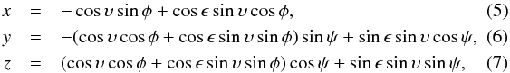$\begin{array}{ccc}\mathit{x}& \mathrm{=}& \mathrm{-}\cos \mathit{\upsilon }\sin \mathit{\phi }\mathrm{+}\cos \mathit{ϵ}\sin \mathit{\upsilon }\cos \mathit{\phi ,}\\ \mathit{y}& \mathrm{=}& \mathrm{-}\mathrm{(}\cos \mathit{\upsilon }\cos \mathit{\phi }\mathrm{+}\cos \mathit{ϵ}\sin \mathit{\upsilon }\sin \mathit{\phi }\mathrm{)}\sin \mathit{\psi }\mathrm{+}\sin \mathit{ϵ}\sin \mathit{\upsilon }\cos \mathit{\psi ,}\\ \mathit{z}& \mathrm{=}& \mathrm{(}\cos \mathit{\upsilon }\cos \mathit{\phi }\mathrm{+}\cos \mathit{ϵ}\sin \mathit{\upsilon }\sin \mathit{\phi }\mathrm{)}\cos \mathit{\psi }\mathrm{+}\sin \mathit{ϵ}\sin \mathit{\upsilon }\sin \mathit{\psi ,}\end{array}$where υ is the angle between the point of the equinox and the direction towards the Sun. (See Appendix A for a detailed derivation.) In these coordinates, the outward normal is n = (0,0,1), and the local meridian is aligned with y-axis.

2.2. Numeric methods

We use a numeric code similar to the one used by Ševeček et al. (2015). The heat diffusion equation is solved using the finite element discretization in space. The temperature is approximated by a linear combination of prescribed basis functions: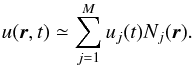$\mathit{u}\mathrm{\left(}{r}\mathit{,t}\mathrm{\right)}\mathrm{\simeq }\sum _{\mathit{j}\mathrm{=}\mathrm{1}}^{\mathit{M}}{\mathit{u}}_{\mathit{j}}\mathrm{\left(}\mathit{t}\mathrm{\right)}{\mathit{N}}_{\mathit{j}}\mathrm{\left(}{r}\mathrm{\right)}\mathit{.}$(8)As for the temporal derivative, we use an implicit Euler scheme with constant time-step. We derive a weak formulation of the problem (see Sect. 2.2 of Ševeček et al. 2015) and we solve the resulting system of linear algebraic equations using the FreeFem++ code (Hecht 2012). The computational domain is prepared from a simple geometry (a spherical boulder in a regolith block) using the tetgen code (Si 2006).

Once we obtain the temperature distribution, we express the magnitude of the torque using the day-averaged dimensionless pressure ⟨ Π ⟩: 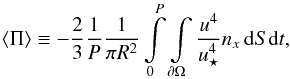$\mathrm{⟨}\mathrm{\Pi }\mathrm{⟩}\mathrm{\equiv }\mathrm{-}\frac{\mathrm{2}}{\mathrm{3}}\frac{\mathrm{1}}{\mathit{P}}\frac{\mathrm{1}}{\mathit{\pi }{\mathit{R}}^{\mathrm{2}}}\underset{\mathrm{0}}{\overset{\mathit{P}}{\mathrm{\int }}}\underset{}{{\mathrm{\int }}^{\mathit{\partial }\mathrm{\Omega }}}\frac{{\mathit{u}}^{\mathrm{4}}}{{\mathit{u}}_{\mathit{\star }}^{\mathrm{4}}}{\mathit{n}}_{\mathit{x}}\hspace{0.17em}\mathrm{d}\mathit{S}\mathrm{d}\mathit{t,}$(9)where P is the rotational period, R is the radius of the spherical boulder, u is the temperature at given point on the surface, ${\mathit{u}}_{\mathit{\star }}\mathrm{\equiv }\mathrm{\left[}\mathrm{\right(}\mathrm{1}\mathrm{-}\mathit{A}\mathrm{)}{\mathrm{\Phi }}_{\mathrm{\odot }}\mathit{/}\mathrm{(}\mathit{\sigma ϵ}\mathrm{)}{\mathrm{]}}^{\frac{\mathrm{1}}{\mathrm{4}}}$ is the subsolar temperature, and n_x is the x-component of the (outward) normal. The negative sign expresses that the pressure acts against the normal, while the coefficient 2/3 comes from integrating over all possible directions of the emitted light, assuming Lambert’s emission indicatrix.

Lastly, we need to account for variations of the torque during its revolution around the Sun. We thus define the year-averaged dimensionless pressure ⟨ ⟨ Π ⟩ ⟩ (or simply the mean dimensionless pressure) 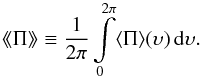$\mathrm{⟨}\mathrm{⟨}\mathrm{\Pi }\mathrm{⟩}\mathrm{⟩}\mathrm{\equiv }\frac{\mathrm{1}}{\mathrm{2}\mathit{\pi }}\underset{\mathrm{0}}{\overset{\mathrm{2}\mathit{\pi }}{\mathrm{\int }}}\mathrm{⟨}\mathrm{\Pi }\mathrm{⟩}\mathrm{\left(}\mathit{\upsilon }\mathrm{\right)}\hspace{0.17em}\mathrm{d}\mathit{\upsilon }\mathit{.}$(10)We note that we assume zero eccentricity and thus can integrate over the angle υ rather than the time. In practice, we evaluate ⟨ Π ⟩ at a finite number of points around the orbit and average these values to estimate the integral.

For our purposes, the mean dimensionless pressure ⟨ ⟨ Π ⟩ ⟩ is the final result. Previous works (Golubov & Krugly 2012; Golubov et al. 2014; Ševeček et al. 2015) discussed the total torque boulders exert on an asteroid and the corresponding change of the angular frequency; in this paper, however, we mainly focus on the dependence of the torque on different parameters rather than on its absolute magnitude, and thus ⟨ ⟨ Π ⟩ ⟩ is a useful quantity for this purpose. The parametric space is quite extended and cannot be studied thoroughly with available computational resources. We thus perform sections through parametric space by varying one parameter and keeping all other parameters constant at reasonable, physically relevant values.

To reach a stationary solution we need to evolve the system for several rotational periods. For low values of ψ and ϵ, the convergence is fast, and only 4−5 periods are required. At high latitudes and obliquities, however, the analytical solution is not a good approximation and up to 50 periods are needed to achieve the same accuracy. Runs requiring the most periods are the ones where the boulder is in the polar night and the Sun does not appear above the horizon during the rotational period at all. However, it is obvious that the pressure ⟨ Π ⟩ will be zero in these cases. Therefore, to save computation time, the boulder is assumed to be in polar night and the run is skipped altogether, if the following condition is met: $\tan \mathit{\psi }\sin \mathit{\upsilon }\sin \mathit{ϵ}\mathrm{\le }\mathrm{-}\sqrt{{\cos }^{\mathrm{2}}\mathit{\upsilon }\mathrm{+}{\cos }^{\mathrm{2}}\mathit{ϵ}{\sin }^{\mathrm{2}}\mathit{\upsilon }}\mathit{.}$(11)We confirmed on a test run that the code will return a negligible pressure of ⟨ Π ⟩ ≃ 10^-7 if the condition (11) is met, even though it takes about 300 periods.

3. Results

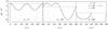Fig. 1 Variations of the day-averaged dimensionless pressure ⟨ Π ⟩ during the revolution around the Sun. Various values of latitude ψ and obliquity ϵ are plotted.

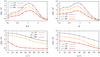Fig. 2 TYORP as a function of relevant parameters. The upper two panels show ⟨ ⟨ Π ⟩ ⟩ for Θ = 1 and different R/L (upper left panel) or R/L = 1 and different Θ (upper right panel), for latitude ψ = 0° in all cases, and for three different values of obliquity ϵ. The lower two panels show ⟨ ⟨ Π ⟩ ⟩ for different values of ϵ and ψ, while both Θ and R/L are set to 1.

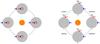Fig. 3 Illustration of TYORP dependence on obliquity ϵ and latitude ψ. Two asteroids are shown, with ϵ ≈ 0° and ϵ ≈ 90°, and two boulders on their surface, with ψ ≈ 0° and ψ ≈ 90°.

Results of our simulations are plotted in Figs. 1, 2, and 4.

Figure 1 illustrates how the overall TYORP torque ⟨ ⟨ Π ⟩ ⟩ is accumulated over time via contributions from different seasons. The season-unaveraged torque ⟨ Π ⟩ is plotted versus υ, the angle the asteroid has passed from the equinox. Three different values of latitude ψ are shown in different panels, and two different values of obliquity ϵ are shown with different lines. For ϵ = 0° the torque ⟨ Π ⟩ is constant as function of υ, but with increasing obliquity the seasonal distribution of ⟨ Π ⟩ gets more uneven. For ψ = 0° equinoxes produce larger contributions than solstices, which is reasonable as an illumination from the East and the West is the most important for TYORP, and this is exactly the type of illumination that is more prominent during equinoxes than during solstices, when more illumination comes from the South (winter solstice) or from above (summer solstice). Everywhere but the equator winter solstices give a smaller contribution than summer solstices. Naturally, ⟨ Π ⟩ is zero during polar nights.

Figure 2 is the central result of this article. It illustrates how the torque ⟨ ⟨ Π ⟩ ⟩ depends on the relevant physical parameters: thermal parameter Θ, non-dimensional radius R/L, obliquity ϵ, and latitude ψ. In each panel only two parameters vary (one is colour-coded, and the other is given on the horizontal axis), while the others are set to two of the following values: Θ = 1, R/L = 1, ψ = 0°. We can imagine ⟨ ⟨ Π ⟩ ⟩ plotted above a four-dimensional parameter space, and Fig. 2 presenting some sections of this space. We only plot obliquities between 0 and 90°, however all of the results should be symmetric about 90°, with results for obliquities of 0 and 180° being the same.

From the upper two panels of Fig. 2, we see that R/L and Θ are separable from ϵ, so that changes in ϵ mostly cause a rescaling of the plot with the same coefficient for all R/L and Θ. Parameters ϵ and ψ are clearly not separable, and a change of ψ causes larger relative changes in TYORP at high obliquities than at low obliquities.

Many features of the dependence of TYORP pressure ⟨ ⟨ Π ⟩ ⟩ on obliquity ϵ and latitude ψ can be understood intuitively from Fig. 3. If an asteroid has zero obliquity, as in the left-hand panel of Fig. 3, then boulders A with ψ ≈ 0° and B with ψ ≈ 90° appear in similar conditions. Although at noon the former is illuminated from above while the latter from the South, in the morning and in the evening illumination conditions are exactly equivalent. Thus it is sensible that the difference between the cases ψ ≈ 0° and ψ ≈ 90° are only about twofold. A larger TYORP effect for ψ ≈ 0° can be attributed to it having a projected area up to two times larger, thus absorbing and emitting more light.

This contrasts with the result by Golubov et al. (2014), who obtained ⟨ ⟨ Π ⟩ ⟩ = 0 when ψ = 90°, which happened as a result of the regular arrangement of stones on the surface they considered, and thus accounted for their mutual shadowing. Here we disregard shadowing and consider only isolated stones. Close to the pole, shadowing is particularly important so that only the tops of spheres are illuminated, creating a negligible TYORP. This puts limitations on the applicability of the model used in this article, but these limitations are of lesser importance as polar regions have a relatively small area, low illumination levels and, in general, smaller lever arms, all of which minimizes their contribution to the total TYORP effect on an asteroid.

We now consider an asteroid with obliquity ϵ = 90°, as in the right-hand panel of Fig. 3. At spring and vernal equinox the boulder A lying at the equator creates the same TYORP as in the previous case with ϵ = 0°, while at solstices it is continuously illuminated from one side (either North or South) and creates no TYORP. During a year different intermediates between these two regimes occur, and the year average should be about one half of the maximal YORP for ϵ = 0°, in accordance with Fig. 2. Stone B, lying close to the north pole, is shadowed during polar night, in autumn and in winter. Shortly after spring equinox, and shortly before vernal equinox, the stone creates the same TYORP as a stone in a polar region of an asteroid with ϵ = 0°, while around summer solstice the stone is perpetually illuminated from above, and creates no TYORP. The mean of about a half of the maximum TYORP for only half a year means the average TYORP for stone B should be about four times smaller than TYORP for a stone in the same position at an asteroid with ϵ = 0°.

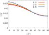Fig. 4 Non-dimensional surface-integrated TYORP torque as a function of obliquity. Different colors correspond to different axis ratios of ellipsoidal asteroids. The grey line corresponds to the formula 0.012(1 + cos2ϵ), which approximates TYORP well for a sphere.

To obtain the overall torque T_z experienced by an asteroid, we need to integrate TYORP over its surface. It is convenient to introduce the non-dimensional torque τ_z by dividing T_z over (1−A)Φ_⊙r³/c, where c is the speed of light, and r is the equivalent radius of the asteroid (Golubov & Krugly 2012). The overall torque also depends on the number of boulders on the surface. Neglecting mutual shadowing of the boulders, τ_z is proportional to their density on the surface of the asteroid n, or to the fraction of the surface area occupied by the boulders, f = πR²n. We compute τ_z/f for ellipsoidal asteroids as described in Appendix B, and plot the results in Fig. 4. We find that the TYORP effect for three asteroids with different shapes is almost the same. The approximate independence of τ_z was predicted using a simplified analytical model in Appendix B of Golubov et al. (2014). For ϵ = 0°, the overall TYORP is nearly twice as big as for ϵ = 90°. This is in a good agreement with the lower two panels in Fig. 2, where roughly the same two-fold difference between ϵ = 0° and ϵ = 90° is present at low latitudes, and it is the low latitudes that contribute the most to τ_z owing to their larger area, larger lever arm, and larger ⟨ ⟨ Π ⟩ ⟩. A simple analytic dependence on latitude with τ_z proportional to 1 + cos²ϵ gives a good fit for a spherical asteroid, and also a reasonable estimate for ellipsoidal asteroids (grey line in Fig. 4). Finally, we note that τ_z/f is nearly nine times larger than ⟨ ⟨ Π ⟩ ⟩ at the equator, and also agrees with Appendix B of Golubov et al. (2014), which predicted the factor between τ_z/f and ⟨ ⟨ Π ⟩ ⟩ to be about nine.

4. Conclusions

We find the TYORP effect to operate for non-zero obliquities, making it a truly general effect. At high obliquities, TYORP only gets a factor of a few smaller. In all the cases tested, TYORP remains positive (see Fig. 2), and even in all seasons the day-averaged contribution to TYORP is also positive in all our simulations (see Fig. 1). The numerical value of TYORP for different latitudes and obliquities has a clear physical explanation (see Fig. 3 and its discussion in the text). The size of boulders and thermal parameters look to be separable from the latitude and obliquity, so that their alteration only causes a rescaling of the plots as a whole. The surface-integrated TYORP torque for an ellipsoidal asteroid at high obliquities is about two times less than for low obliquities, with the law τ_z ∝ 1 + cos²ϵ providing a crude estimate (Fig. 4). Its value and its weak dependence on the shape of the asteroid are in good agreement with

the rough analytic estimates by Golubov et al. (2014). The development of these simple models for the TYORP effect enable it to be generally incorporated into more detailed evolutionary models of asteroid rotation when subject to solar illumination effects.

Acknowledgments

O.G. and D.J.S. acknowledge support from NASA grant NNX14AL16G from the Near-Earth Object Observation Program and from grants from NASA’s SSERVI Institute.

References

Appendix A: Sun coordinates

Figure A.1 shows different coordinate systems. Sun in a reference frame co-moving with the asteroid has coordinates $\begin{array}{ccc}\mathit{x}& \mathrm{=}& \cos \mathit{\upsilon ,}\\ \mathit{y}& \mathrm{=}& \cos \mathit{ϵ}\sin \mathit{\upsilon ,}\\ \mathit{z}& \mathrm{=}& \end{array}$where ϵ is the obliquity and υ is the angle between the point of the equinox and the direction towards the Sun. In a co-rotating frame, we have $\begin{array}{ccc}{\mathit{x}}^{\mathrm{\prime }}& \mathrm{=}& \cos \mathit{\upsilon }\cos \mathit{\phi }\mathrm{+}\cos \mathit{ϵ}\sin \mathit{\upsilon }\sin \mathit{\phi ,}\\ {\mathit{y}}^{\mathrm{\prime }}& \mathrm{=}& \mathrm{-}\cos \mathit{\upsilon }\sin \mathit{\phi }\mathrm{+}\cos \mathit{ϵ}\sin \mathit{\upsilon }\cos \mathit{\phi ,}\\ {\mathit{z}}^{\mathrm{\prime }}& \mathrm{=}& \end{array}$where φ = ωt, ω being the rotational frequency.

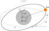Fig. A.1 Different coordinate systems used in the article and angles between their axes.

Finally, we get the Sun coordinates in a local coordinate system of a boulder by rotating around the y′ axis by the latitude ψ: $\begin{array}{ccc}{\mathit{x}}^{\mathrm{\prime \prime }}& \mathrm{=}& \mathrm{(}\cos \mathit{\upsilon }\cos \mathit{\phi }\mathrm{+}\cos \mathit{ϵ}\sin \mathit{\upsilon }\sin \mathit{\phi }\mathrm{)}\cos \mathit{\psi }\mathrm{+}\sin \mathit{ϵ}\sin \mathit{\upsilon }\sin \mathit{\psi }\\ {\mathit{y}}^{\mathrm{\prime \prime }}& \mathrm{=}& \mathrm{-}\cos \mathit{\upsilon }\sin \mathit{\phi }\mathrm{+}\cos \mathit{ϵ}\sin \mathit{\upsilon }\cos \mathit{\phi }\\ {\mathit{z}}^{\mathrm{\prime \prime }}& \mathrm{=}& \mathrm{-}\mathrm{(}\cos \mathit{\upsilon }\cos \mathit{\phi }\mathrm{+}\cos \mathit{ϵ}\sin \mathit{\upsilon }\sin \mathit{\phi }\mathrm{)}\sin \mathit{\psi }\mathrm{+}\sin \mathit{ϵ}\sin \mathit{\upsilon }\cos \mathit{\psi }\end{array}$

In this local coordinate system, x′′ axis is a local (outward) normal, z′′ has a direction of a local meridian and y′′ completes a right-handed orthonormal system. Lastly, we simply rename axes so that the z is now the local normal, for convenience.

Appendix B: Integration of TYORP over the surface

Let the asteroid be triaxial ellipsoid with axes a ≥ b ≥ c. We parameterize radius vector belonging to its surface as ${r}\mathrm{=}\mathrm{\left(}\mathit{a}\sin \mathit{\theta }\cos \mathit{\alpha ,b}\sin \mathit{\theta }\sin \mathit{\alpha ,c}\cos \mathit{\theta }\mathrm{\right)}\mathit{,}$(B.1)where the parameters θ and α are constrained to the ranges 0 ≤ θ ≤ π and 0 ≤ α ≤ 2π. Then we take a small surface element, corresponding to small changes of the parameters, Δθ and Δα. Two edges of this area are found via partial derivatives of r over θ and α, and their vector product gives the vector surface area ${\Delta }{S}\mathrm{=}\mathrm{\left(}\mathit{bc}\sin \mathit{\theta }\cos \mathit{\alpha ,ac}\sin \mathit{\theta }\sin \mathit{\alpha ,ab}\cos \mathit{\theta }\mathrm{\right)}\sin \mathit{\theta }\hspace{0.17em}\mathrm{\Delta }\mathit{\theta }\hspace{0.17em}\mathrm{\Delta }\mathit{\alpha }\mathit{.}$(B.2)We find the surface area from the length of this vector, and the latitude ψ from its orientation. (The latter is necessary to compute ⟨ ⟨ Π ⟩ ⟩.)

To find the lever arm of the TYORP force, we project r and ΔS over the equatorial plane, construct a line in this plane crossing through the projection of r and perpendicular to the projection of ΔS, and find the distance from the origin to this line. Thus we get the lever arm $\mathit{L}\mathrm{=}\frac{\mathit{ab}\sin \mathit{\theta }}{\sqrt{{\mathit{a}}^{\mathrm{2}}{\sin }^{\mathrm{2}}\mathit{\alpha }\mathrm{+}{\mathit{b}}^{\mathrm{2}}{\cos }^{\mathrm{2}}\mathit{\alpha }}}\mathrm{·}$(B.3)Finally, the TYORP torque is obtained by numerically adding up the torques created by all surface elements, ${\mathit{T}}_{\mathit{z}}\mathrm{=}\frac{\mathrm{(}\mathrm{1}\mathrm{-}\mathit{A}\mathrm{)}{\mathrm{\Phi }}_{\mathrm{\odot }}\mathit{f}}{\mathit{C}}\begin{array}{c}\sum \end{array}\mathrm{⟨}\mathrm{⟨}\mathrm{\Pi }\mathrm{⟩}\mathrm{⟩}\hspace{0.17em}\mathit{L}\hspace{0.17em}\mathrm{\Delta }\mathit{S,}$(B.4)where C is the speed of light, and f is the fraction of the surface occupied by the stones.

Values of φ are different for different facets, and ⟨ ⟨ Π ⟩ ⟩ depends on them. As we have only pre-computed ⟨ ⟨ Π ⟩ ⟩ for a small set of values of φ, we interpolate between the points using Lagrange polynomials. This is intentionally constructed to be symmetric with respect to the equatorial plane, which makes the obtained dependence more physical and the final result more accurate.

The final TYORP torque is non-dimensionalized as ${\mathit{\tau }}_{\mathit{z}}\mathrm{=}\frac{{\mathit{T}}_{\mathit{z}}\mathit{C}}{\mathrm{(}\mathrm{1}\mathrm{-}\mathit{A}\mathrm{)}{\mathrm{\Phi }}_{\mathrm{\odot }}{\mathit{r}}^{\mathrm{3}}}\mathrm{=}\frac{\mathit{f}}{\mathit{abc}}\begin{array}{c}\sum \end{array}\mathrm{⟨}\mathrm{⟨}\mathrm{\Pi }\mathrm{⟩}\mathrm{⟩}\hspace{0.17em}\mathit{L}\hspace{0.17em}\mathrm{\Delta }\mathit{S}\mathit{.}$(B.5)

All Figures

	Fig. 1 Variations of the day-averaged dimensionless pressure ⟨ Π ⟩ during the revolution around the Sun. Various values of latitude ψ and obliquity ϵ are plotted.
In the text

	Fig. 2 TYORP as a function of relevant parameters. The upper two panels show ⟨ ⟨ Π ⟩ ⟩ for Θ = 1 and different R/L (upper left panel) or R/L = 1 and different Θ (upper right panel), for latitude ψ = 0° in all cases, and for three different values of obliquity ϵ. The lower two panels show ⟨ ⟨ Π ⟩ ⟩ for different values of ϵ and ψ, while both Θ and R/L are set to 1.
In the text

	Fig. 3 Illustration of TYORP dependence on obliquity ϵ and latitude ψ. Two asteroids are shown, with ϵ ≈ 0° and ϵ ≈ 90°, and two boulders on their surface, with ψ ≈ 0° and ψ ≈ 90°.
In the text

	Fig. 4 Non-dimensional surface-integrated TYORP torque as a function of obliquity. Different colors correspond to different axis ratios of ellipsoidal asteroids. The grey line corresponds to the formula 0.012(1 + cos2ϵ), which approximates TYORP well for a sphere.
In the text

	Fig. A.1 Different coordinate systems used in the article and angles between their axes.
In the text

References

- Bottke, W. F., Vokrouhlický, D., Rubincam, D. P., & Nesvorný, D. 2006, AREPS, 34, 157 [NASA ADS] [Google Scholar]
- Golubov, O., & Krugly, Yu. N. 2012, ApJ, 752, L11 [NASA ADS] [CrossRef] [Google Scholar]
- Golubov, O., Scheeres, D. J., & Krugly, Yu. N. 2014, ApJ, 794, 22 [NASA ADS] [CrossRef] [Google Scholar]
- Hecht, F. 2012, J. Num. Math., 20, 251 [Google Scholar]
- Rubincam, D. P. 2000, Icarus 148, 2 [Google Scholar]
- Ševeček, P., Brož, M., Čapek, D., & Ďurech, J. 2015,MNRAS, 450, 2104 [Google Scholar]
- Si, H. 2006. TetGen – A Quality Tetrahedral Mesh Generator and Three-Dimensional Delaunay Triangulator, http://tetgen.berlios.de/ [Google Scholar]
- Vokrouhlický, D., Bottke, W. F., Chesley, S. R., Scheeres, D. J., & Statler, T. S. 2015, in Asteroids IV, eds. P. Michel, F. E. DeMeo, & W. F. Bottke (Tucson: University of Arizona Press), 509 [Google Scholar]