© ESO, 2016

1. Introduction

Weak gravitational lensing based on shear measurements is challenging because an unbiased estimate of the shear must be obtained from the observed images of faint distant galaxies (see, e.g., Heymans et al. 2006; Massey et al. 2007; Mandelbaum et al. 2015). Biases in shear estimates are commonly parametrized through $\mathit{\gamma ̂}\mathrm{=}\mathrm{(}\mathrm{1}\mathrm{+}\mathit{m}\mathrm{)}\mathit{\gamma }\mathrm{+}\mathit{c,}$(1)where is the expectation value of the shear estimate, γ is the true shear – a two-component quantity, conveniently written as a complex number – and m and c are the multiplicative and additive biases, respectively. The additive bias itself is a complex quantity and thus has a phase (or an orientation). As such, it defines a direction on the sky. The presence of an additive bias can thus be detected by correlating the estimated shear with other quantities that define directions, such as the phase of the point-spread function (PSF) for which any shape measurement must be corrected, signaling an incomplete PSF-correction, or the pixel grid of the detector. For the rest of the letter, we ignore the additive bias parameter.

In contrast to c, a multiplicative bias cannot be easily identified in the data themselves. Such a bias is expected to arise from the smearing correction of the PSF, pixelization, pixel noise (“noise bias”; e.g., Melchior & Viola 2012; Bartelmann et al. 2012), and, depending on the method used for shear estimates, insufficient knowledge of the distribution of intrinsic brightness profiles of sources (“underfitting bias”, or “model bias”, e.g., Voigt & Bridle 2010; Bernstein 2010; Miller et al. 2013; Bernstein & Armstrong 2014; Schneider et al. 2015, and references therein).

An absolute determination of m from the data therefore appears extremely challenging. Possible methods for this include the use of magnification information (Rozo & Schmidt 2010), or the calibration of shear as measured from faint galaxy images with the shear obtained from the lensed cosmic microwave background (Das et al. 2013). If the multiplicative bias depends on galaxy properties, such as color or size, then a relative bias may be detected in the data by splitting the galaxy sample and comparing the results.

In this letter, we propose a new method for detecting a redshift-dependent multiplicative bias, which we call generalized shear-ratio test (GSRT). It is a purely geometrical method, based on a relation between distances in (statistically) isotropic universes, which we derive in Sect.3. In contrast to the classical shear-ratio test (see Sect.2), which yields a geometrical probe of the cosmological model assuming no multiplicative bias, the GSRT is independent of the cosmological model and even independent of the validity of Einstein’s field equation, but capable of detecting the redshift-dependent bias m, as we describe in Sect.4. Furthermore, we derive a relation between shear ratios that is even independent of a multiplicative bias, but only depends on the redshifts of lens and source populations. As such, this relation offers the opportunity of studying the accuracy of photometric redshifts in cosmological weak-lensing surveys.

2. Classical shear-ratio test

Any observable weak-lensing quantity that is linear in the shear depends linearly on the surface mass density Σ of the lens (see, e.g., Bartelmann & Schneider 2001; Kilbinger 2015). For a lens (or a population of lenses) at redshift z₁ and a source population at redshift z₂, such a shear quantity S can be expressed as $\mathit{S}\mathrm{=}\mathit{G}\frac{\mathit{D}\mathrm{\left(}{\mathit{z}}_{\mathrm{1}}\mathit{,}{\mathit{z}}_{\mathrm{2}}\mathrm{\right)}}{\mathit{D}\mathrm{\left(}{\mathit{z}}_{\mathrm{2}}\mathrm{\right)}}\mathrm{\equiv }\mathit{G}\hspace{0.17em}\mathit{\beta }\mathrm{\left(}{\mathit{z}}_{\mathrm{1}}\mathit{,}{\mathit{z}}_{\mathrm{2}}\mathrm{\right)}\mathit{,}$(2)where D(z₁,z₂) is the angular-diameter distance of the sources at z₂ as seen from an observer at z₁, and D(z₂) ≡ D(0,z₂) is the angular-diameter distance of the sources from us. The lensing quantity G is linear in the scaled dimensionless surface mass density ${\mathit{\kappa }}_{\mathrm{sc}}\mathrm{=}\frac{\mathrm{4}\mathit{\pi G}}{{\mathit{c}}^{\mathrm{2}}}\hspace{0.17em}\mathit{D}\mathrm{\left(}{\mathit{z}}_{\mathrm{1}}\mathrm{\right)}\hspace{0.17em}\mathrm{\Sigma }\mathit{,}$(3)and depends solely on the properties and distance of the lens (population), but is independent of the source redshift. In Eq.(2), we have defined the distance ratio β, which for a given lens characterizes the lensing strength as a function of source redshift.

The true image ellipticity ϵ of a background galaxy is an unbiased estimate of the reduced shear γ/ (1−κ) (Seitz & Schneider 1997), where κ = κ_scβ(z₁,z₂) is the convergence of the lens at z₁ for a source population at redshift z₂. Assuming that the convergence is much smaller than unity, we neglect the difference between shear and reduced shear; indeed, the lensing quantity G may be chosen such that it avoids shear measurements in close neighborhood of lenses, which not only reduces the difference between γ and g, but also avoids potential difficulties with photometry of closely spaced objects (in this case, lens and source).

Then, an estimate of S is obtained as a linear combination of image ellipticities ϵ, whose expectation value is $\mathrm{\Gamma }\mathrm{\left(}{\mathit{z}}_{\mathrm{1}}\mathit{,}{\mathit{z}}_{\mathrm{2}}\mathrm{\right)}\mathrm{=}\mathit{G}\mathrm{\left(}{\mathit{z}}_{\mathrm{1}}\mathrm{\right)}\hspace{0.17em}\mathit{\beta }\mathrm{\left(}{\mathit{z}}_{\mathrm{1}}\mathit{,}{\mathit{z}}_{\mathrm{2}}\mathrm{\right)}\hspace{0.17em}\mathit{M}\mathrm{\left(}{\mathit{z}}_{\mathrm{2}}\mathrm{\right)}\mathit{,}$(4)where M = (1 + m), with m being the aforementioned multiplicative bias in shear measurements. For example, Γ(z₁,z₂) could be a weighted integral over separation of the tangential shear in galaxy-galaxy lensing for lenses at z₁, measured for sources at z₂, where the weight can be chosen such as to optimize the signal-to-noise ratio of the measurement (e.g., Bartelmann & Schneider 2001).

Hence, the observable signal Γ depends (i) on the properties of the lens described by G; (ii) on the cosmological model through the distance ratio β; and (iii) on the multiplicative bias in shear measurements. Furthermore; it also depends (iv) on the reliability of the estimates of (photometric) redshifts.

The classical shear-ratio test (Jain & Taylor 2003; Taylor et al. 2007; Kitching et al. 2016) considers a lens (population) at redshift z₁, and two source populations at redshifts z₂ and z₃. The ratio of their lensing signals, $\mathit{R}\mathrm{\left(}{\mathit{z}}_{\mathrm{1}}\mathrm{;}{\mathit{z}}_{\mathrm{2}}\mathit{,}{\mathit{z}}_{\mathrm{3}}\mathrm{\right)}\mathrm{\equiv }\frac{\mathrm{\Gamma }\mathrm{\left(}{\mathit{z}}_{\mathrm{1}}\mathit{,}{\mathit{z}}_{\mathrm{3}}\mathrm{\right)}}{\mathrm{\Gamma }\mathrm{\left(}{\mathit{z}}_{\mathrm{1}}\mathit{,}{\mathit{z}}_{\mathrm{2}}\mathrm{\right)}}\mathrm{=}\frac{\mathit{\beta }\mathrm{\left(}{\mathit{z}}_{\mathrm{1}}\mathit{,}{\mathit{z}}_{\mathrm{3}}\mathrm{\right)}}{\mathit{\beta }\mathrm{\left(}{\mathit{z}}_{\mathrm{1}}\mathit{,}{\mathit{z}}_{\mathrm{2}}\mathrm{\right)}}\hspace{0.17em}\frac{\mathit{M}\mathrm{\left(}{\mathit{z}}_{\mathrm{3}}\mathrm{\right)}}{\mathit{M}\mathrm{\left(}{\mathit{z}}_{\mathrm{2}}\mathrm{\right)}}\mathrm{\equiv }\mathit{B}\mathrm{\left(}{\mathit{z}}_{\mathrm{1}}\mathrm{;}{\mathit{z}}_{\mathrm{2}}\mathit{,}{\mathit{z}}_{\mathrm{3}}\mathrm{\right)}\hspace{0.17em}\frac{\mathit{M}\mathrm{\left(}{\mathit{z}}_{\mathrm{3}}\mathrm{\right)}}{\mathit{M}\mathrm{\left(}{\mathit{z}}_{\mathrm{2}}\mathrm{\right)}}\mathit{,}$(5)eliminates the dependence on the lens properties. Owing to its dependence on the distance ratio B, the shear ratio R was proposed as a probe for cosmological parameters. However, the sensitivity of B on the equation-of-state parameter w of dark energy, for example, turns out to be rather weak, so that highly accurate measurements of R are needed to turn this into a competitive cosmological probe. Furthermore, unbiased estimates of shear and redshifts that enter the shear ratio test provide a great challenge for precision weak-lensing experiments. It is therefore of great interest to find observational probes for a potential multiplicative bias in shear measurements and a bias of photometric redshifts that is insensitive to assumptions about the cosmological parameters.

In the next section, we derive relations between cosmological distances that are independent of cosmological parameters and allow us to construct combinations of R that no longer carry a dependence on cosmology.

3. Distance relation in isotropic universes

The two-dimensional separation vector ξ between two infinitesimally close light rays follows the geodesic deviation equation $\frac{{\mathrm{d}}^{\mathrm{2}}{\xi }}{\mathrm{d}{\mathit{\lambda }}^{\mathrm{2}}}\mathrm{=}\mathrm{𝒯}\mathrm{\left(}\mathit{\lambda }\mathrm{\right)}\hspace{0.17em}{\xi }\mathrm{\left(}\mathit{\lambda }\mathrm{\right)}\mathit{,}$(6)where λ is the affine parameter along the light rays, and is the optical tidal matrix, which is determined by the Ricci and Weyl tensors of the spacetime metric (see, e.g., Chap.3 of Schneider et al. 1992; Seitz et al. 1994). In an isotropic universe, the tidal part of vanishes, so that , where ℐ is the two-dimensional unit matrix and T(λ) is a scalar function, proportional to the local density.

If the two light rays intersect at a vertex at λ_i under an angle θ, we can write ξ(λ) = D_i(λ)θ, where D_i satisfies the differential equation 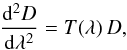$\frac{{\mathrm{d}}^{\mathrm{2}}\mathit{D}}{\mathrm{d}{\mathit{\lambda }}^{\mathrm{2}}}\mathrm{=}\mathit{T}\mathrm{\left(}\mathit{\lambda }\mathrm{\right)}\hspace{0.17em}\mathit{D,}$(7)with initial conditions D_i(λ_i) = 0, (dD_i/ dλ)(λ_i) = Ḋ_i, where the latter value depends on the choice of the affine parameter. By definition, D_i(λ) is the angular-diameter distance of a source at λ, seen from an observer at λ_i<λ.

The second-order differential Eq. (7) has two independent solutions; we chose them to be D_i(λ) and D_j(λ), that is, the angular-diameter distances as measured from observers located at λ_i and λ_j ≠ λ_i, respectively. A third solution, D_k(λ), must necessarily be a linear combination of the other two. If we write it in the form

${\mathit{D}}_{\mathit{k}}\mathrm{\left(}\mathit{\lambda }\mathrm{\right)}\mathrm{=}\mathit{C}\mathrm{\left[}{\mathit{D}}_{\mathit{j}}\mathrm{\right(}\mathit{\lambda }\mathrm{\left)}{\mathit{D}}_{\mathit{i}}\mathrm{\right(}{\mathit{\lambda }}_{\mathit{k}}\mathrm{)}\mathrm{-}{\mathit{D}}_{\mathit{j}}\mathrm{(}{\mathit{\lambda }}_{\mathit{k}}\mathrm{\left)}{\mathit{D}}_{\mathit{i}}\mathrm{\right(}\mathit{\lambda }{\mathrm{\left)}}^{\mathrm{\right]}}\mathit{,}$where C is a constant, then we see that the first initial condition is satisfied, D_k(λ_k) = 0. For the second initial condition, we have 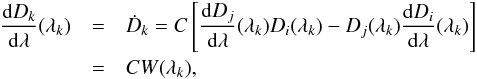$\begin{array}{ccc}\frac{\mathrm{d}{\mathit{D}}_{\mathit{k}}}{\mathrm{d}\mathit{\lambda }}\mathrm{\left(}{\mathit{\lambda }}_{\mathit{k}}\mathrm{\right)}& \mathrm{=}& \mathit{Ḋ}\mathit{k}\mathrm{=}\mathit{C}\left[\frac{\mathrm{d}{\mathit{D}}_{\mathit{j}}}{\mathrm{d}\mathit{\lambda }}\mathrm{\left(}{\mathit{\lambda }}_{\mathit{k}}\mathrm{\right)}{\mathit{D}}_{\mathit{i}}\mathrm{\left(}{\mathit{\lambda }}_{\mathit{k}}\mathrm{\right)}\mathrm{-}{\mathit{D}}_{\mathit{j}}\mathrm{\left(}{\mathit{\lambda }}_{\mathit{k}}\mathrm{\right)}\frac{\mathrm{d}{\mathit{D}}_{\mathit{i}}}{\mathrm{d}\mathit{\lambda }}\mathrm{\left(}{\mathit{\lambda }}_{\mathit{k}}\mathrm{\right)}\right]\\ & \mathrm{=}& \end{array}$(8)where W(λ) is the Wronskian

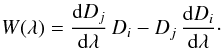$\mathit{W}\mathrm{\left(}\mathit{\lambda }\mathrm{\right)}\mathrm{=}\frac{\mathrm{d}{\mathit{D}}_{\mathit{j}}}{\mathrm{d}\mathit{\lambda }}\hspace{0.17em}{\mathit{D}}_{\mathit{i}}\mathrm{-}{\mathit{D}}_{\mathit{j}}\hspace{0.17em}\frac{\mathrm{d}{\mathit{D}}_{\mathit{i}}}{\mathrm{d}\mathit{\lambda }}\mathrm{·}$From Eq.(7), we directly see that dW/ dλ = 0, i.e., W(λ) is constant. We can calculate this constant considering W at λ_j, which yields

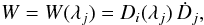$\mathit{W}\mathrm{=}\mathit{W}\mathrm{\left(}{\mathit{\lambda }}_{\mathit{j}}\mathrm{\right)}\mathrm{=}{\mathit{D}}_{\mathit{i}}\mathrm{\left(}{\mathit{\lambda }}_{\mathit{j}}\mathrm{\right)}\hspace{0.17em}\mathit{Ḋ}\mathit{j}\mathit{,}$yielding 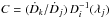$\mathit{C}\mathrm{=}\mathrm{(}\mathit{Ḋ}{}_{\mathit{k}}\mathit{/}\mathit{Ḋ}{}_{\mathit{j}}\mathrm{)}\hspace{0.17em}{\mathit{D}}_{\mathit{i}}^{-1}\mathrm{\left(}{\mathit{\lambda }}_{\mathit{j}}\mathrm{\right)}$. Therefore, 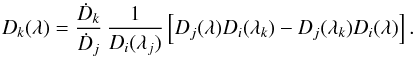${\mathit{D}}_{\mathit{k}}\mathrm{\left(}\mathit{\lambda }\mathrm{\right)}\mathrm{=}\frac{\mathit{Ḋ}\mathit{k}}{\mathit{Ḋ}\mathit{j}}\hspace{0.17em}\frac{\mathrm{1}}{{\mathit{D}}_{\mathit{i}}\mathrm{\left(}{\mathit{\lambda }}_{\mathit{j}}\mathrm{\right)}}\mathrm{\left[}{\mathit{D}}_{\mathit{j}}\mathrm{\right(}\mathit{\lambda }\mathrm{\left)}{\mathit{D}}_{\mathit{i}}\mathrm{\right(}{\mathit{\lambda }}_{\mathit{k}}\mathrm{)}\mathrm{-}{\mathit{D}}_{\mathit{j}}\mathrm{(}{\mathit{\lambda }}_{\mathit{k}}\mathrm{\left)}{\mathit{D}}_{\mathit{i}}\mathrm{\right(}\mathit{\lambda }{\mathrm{\left)}}^{\mathrm{\right]}}\mathit{.}$(9)Thus, we have expressed the angular-diameter distance as seen from an observer at affine parameter λ_k by the corresponding expression for the angular-diameter distance for observers at λ_i and λ_j. The resulting expression contains the initial conditions at λ_j and λ_k. If we now specialize Eq.(9) to the case of λ_i = 0, with the corresponding angular-diameter distance denoted as D(λ), we obtain 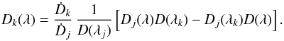${\mathit{D}}_{\mathit{k}}\mathrm{\left(}\mathit{\lambda }\mathrm{\right)}\mathrm{=}\frac{\mathit{Ḋ}\mathit{k}}{\mathit{Ḋ}\mathit{j}}\hspace{0.17em}\frac{\mathrm{1}}{\mathit{D}\mathrm{\left(}{\mathit{\lambda }}_{\mathit{j}}\mathrm{\right)}}\mathrm{\left[}{\mathit{D}}_{\mathit{j}}\mathrm{\right(}\mathit{\lambda }\mathrm{\left)}\mathit{D}\mathrm{\right(}{\mathit{\lambda }}_{\mathit{k}}\mathrm{)}\mathrm{-}{\mathit{D}}_{\mathit{j}}\mathrm{(}{\mathit{\lambda }}_{\mathit{k}}\mathrm{\left)}\mathit{D}\mathrm{\right(}\mathit{\lambda }{\mathrm{\left)}}^{\mathrm{\right]}}\mathit{.}$(10)Combining Eqs.(9) and (10), we then find 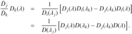$\begin{array}{ccc}\frac{\mathit{Ḋ}\mathit{j}}{\mathit{Ḋ}\mathit{k}}\hspace{0.17em}{\mathit{D}}_{\mathit{k}}\mathrm{\left(}\mathit{\lambda }\mathrm{\right)}& \mathrm{=}& \frac{\mathrm{1}}{{\mathit{D}}_{\mathit{i}}\mathrm{\left(}{\mathit{\lambda }}_{\mathit{j}}\mathrm{\right)}}\mathrm{[}{\mathit{D}}_{\mathit{j}}\mathrm{\left(}\mathit{\lambda }\mathrm{\right)}{\mathit{D}}_{\mathit{i}}\mathrm{\left(}{\mathit{\lambda }}_{\mathit{k}}\mathrm{\right)}\mathrm{-}{\mathit{D}}_{\mathit{j}}\mathrm{\left(}{\mathit{\lambda }}_{\mathit{k}}\mathrm{\right)}{\mathit{D}}_{\mathit{i}}\mathrm{(}\mathit{\lambda }{\mathrm{)}}^{\mathrm{]}}\\ & \mathrm{=}& \end{array}$(11)The final equality no longer contains the initial conditions. It is valid for any spacetime that is isotropic around the observer through which the radial light bundle passes. Furthermore, this equation does not refer to the Einstein field equation and is therefore independent of the validity of General Relativity, as long a spacetime is characterized by a metric. A more graphical derivation of the result (11) is given in Schneider (2016).

If, in addition to isotropy, we assume a spatially homogeneous spacetime, which can then be expressed in the form of the Robertson–Walker metric, the initial conditions are Ḋ_i = (1 + z_i), where z_i is the redshift with which sources at λ_i are seen by the observer at λ = 0 (or redshift zero). For this, we chose a parametrization of the affine parameter such that it locally coincides with the comoving distance as seen from the observer. In what follows, we assume that the isotropic universe is such that an invertible relation between affine parameter and redshift exists, so that redshift can be used to label the relative order of objects (in the sense that an object at z₂ lies behind one at z₁<z₂). This excludes bouncing models, for example, for which z(λ) is not a monotonic function.

We now identify D_i(λ_j) as the distance D(z_i,z_j), and D(λ_j) as D(z_j), that is, the quantities occurring in the distance ratio β (see Eq.(2)). Setting λ = λ_l in Eq.(11) and dividing the resulting expression by D_kD_l, we obtain with the definition (2) that 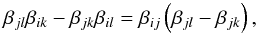${\mathit{\beta }}_{\mathit{jl}}{\mathit{\beta }}_{\mathit{ik}}\mathrm{-}{\mathit{\beta }}_{\mathit{jk}}{\mathit{\beta }}_{\mathit{il}}\mathrm{=}{\mathit{\beta }}_{\mathit{ij}}\mathrm{(}{\mathit{\beta }}_{\mathit{jl}}\mathrm{-}{\mathit{\beta }}_{\mathit{jk}}\mathrm{)}\mathit{,}$(12)an expression between distance ratios β_ij ≡ β(z_i,z_j). This can be manipulated, by division through β_ijβ_jk, to contain just ratios of βs with the first index being the same – or if we set 0 ≤ z_i<z_j<z_k,z_l, with the lower redshift being the same. Hence, the resulting expression only contains the ratios B that were defined in Eq.(5), 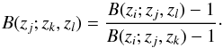$\mathit{B}\mathrm{\left(}{\mathit{z}}_{\mathit{j}}\mathrm{;}{\mathit{z}}_{\mathit{k}}\mathit{,}{\mathit{z}}_{\mathit{l}}\mathrm{\right)}\mathrm{=}\frac{\mathit{B}\mathrm{\left(}{\mathit{z}}_{\mathit{i}}\mathrm{;}{\mathit{z}}_{\mathit{j}}\mathit{,}{\mathit{z}}_{\mathit{l}}\mathrm{\right)}\mathrm{-}\mathrm{1}}{\mathit{B}\mathrm{\left(}{\mathit{z}}_{\mathit{i}}\mathrm{;}{\mathit{z}}_{\mathit{j}}\mathit{,}{\mathit{z}}_{\mathit{k}}\mathrm{\right)}\mathrm{-}\mathrm{1}}\mathrm{·}$(13)Of course, the relation (12) or (13) must hold in a Robertson–Walker metric. The proof of this is outlined in the Appendix.

4. Generalized shear ratio tests

The relation between distances, as derived in the previous section, can now be used to obtain ratios between shear observables Γ. According to Eq.(5), shear ratios depend on the ratios of multiplicative bias factors, hence they cannot be used to determine the absolute multiplicative bias, but only their relative values.

Consider now two populations of lenses at redshifts z₁ and z₂, and sources at redshifts z₂, z₃ and z₄. Combining Eq.(5) with Eq.(13), setting (i,j,k,l) = (1,2,3,4), we find that 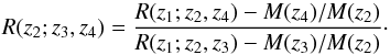$\mathit{R}\mathrm{\left(}{\mathit{z}}_{\mathrm{2}}\mathrm{;}{\mathit{z}}_{\mathrm{3}}\mathit{,}{\mathit{z}}_{\mathrm{4}}\mathrm{\right)}\mathrm{=}\frac{\mathit{R}\mathrm{\left(}{\mathit{z}}_{\mathrm{1}}\mathrm{;}{\mathit{z}}_{\mathrm{2}}\mathit{,}{\mathit{z}}_{\mathrm{4}}\mathrm{\right)}\mathrm{-}\mathit{M}\mathrm{\left(}{\mathit{z}}_{\mathrm{4}}\mathrm{\right)}\mathit{/}\mathit{M}\mathrm{\left(}{\mathit{z}}_{\mathrm{2}}\mathrm{\right)}}{\mathit{R}\mathrm{\left(}{\mathit{z}}_{\mathrm{1}}\mathrm{;}{\mathit{z}}_{\mathrm{2}}\mathit{,}{\mathit{z}}_{\mathrm{3}}\mathrm{\right)}\mathrm{-}\mathit{M}\mathrm{\left(}{\mathit{z}}_{\mathrm{3}}\mathrm{\right)}\mathit{/}\mathit{M}\mathrm{\left(}{\mathit{z}}_{\mathrm{2}}\mathrm{\right)}}\mathrm{·}$(14)This relation between ratios of shear observables is independent of the cosmological model and the validity of the field equation of General Relativity, and contains only ratios of the multiplicative bias at the three source redshifts. Hence we have found a cosmology-independent shear ratio test. The special form of Eq.(14) has been chosen by assuming that the sources at the nearest redshift (here z₂) can be measured most reliably, since these sources probably will on average be larger than those at higher redshift. Thus, we normalize the multiplicative bias by that for sources at z₂.

The redshift dependence may not be the primary dependence of the multiplicative bias; it might instead be suspected that it depends on image size, signal-to-noise ratio, galaxy color, etc. These dependencies can be studied by splitting the source sample. A test based on Eq.(14) may serve as an additional or complementary sanity check.

Furthermore, we can consider three lens populations at redshift z₁, z₂, and z₃, and three source populations at z₃, z₄, and z₅. Replacing (1,2,3,4) → (1,3,4,5) in Eq.(14), we find with Eq.(5) that $\mathit{R}\mathrm{\left(}{\mathit{z}}_{\mathrm{3}}\mathrm{;}{\mathit{z}}_{\mathrm{4}}\mathit{,}{\mathit{z}}_{\mathrm{5}}\mathrm{\right)}\left[\mathit{R}\mathrm{\left(}{\mathit{z}}_{\mathrm{1}}\mathrm{;}{\mathit{z}}_{\mathrm{3}}\mathit{,}{\mathit{z}}_{\mathrm{4}}\mathrm{\right)}\mathrm{-}\frac{\mathit{M}\mathrm{\left(}{\mathit{z}}_{\mathrm{4}}\mathrm{\right)}}{\mathit{M}\mathrm{\left(}{\mathit{z}}_{\mathrm{3}}\mathrm{\right)}}\right]\mathrm{=}\mathit{R}\mathrm{\left(}{\mathit{z}}_{\mathrm{1}}\mathrm{;}{\mathit{z}}_{\mathrm{3}}\mathit{,}{\mathit{z}}_{\mathrm{5}}\mathrm{\right)}\mathrm{-}\frac{\mathit{M}\mathrm{\left(}{\mathit{z}}_{\mathrm{5}}\mathrm{\right)}}{\mathit{M}\mathrm{\left(}{\mathit{z}}_{\mathrm{3}}\mathrm{\right)}}\mathrm{·}$(15)On the other hand, by replacing (1,2,3,4) → (2,3,4,5), we obtain 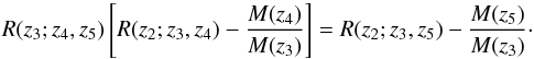$\mathit{R}\mathrm{\left(}{\mathit{z}}_{\mathrm{3}}\mathrm{;}{\mathit{z}}_{\mathrm{4}}\mathit{,}{\mathit{z}}_{\mathrm{5}}\mathrm{\right)}\left[\mathit{R}\mathrm{\left(}{\mathit{z}}_{\mathrm{2}}\mathrm{;}{\mathit{z}}_{\mathrm{3}}\mathit{,}{\mathit{z}}_{\mathrm{4}}\mathrm{\right)}\mathrm{-}\frac{\mathit{M}\mathrm{\left(}{\mathit{z}}_{\mathrm{4}}\mathrm{\right)}}{\mathit{M}\mathrm{\left(}{\mathit{z}}_{\mathrm{3}}\mathrm{\right)}}\right]\mathrm{=}\mathit{R}\mathrm{\left(}{\mathit{z}}_{\mathrm{2}}\mathrm{;}{\mathit{z}}_{\mathrm{3}}\mathit{,}{\mathit{z}}_{\mathrm{5}}\mathrm{\right)}\mathrm{-}\frac{\mathit{M}\mathrm{\left(}{\mathit{z}}_{\mathrm{5}}\mathrm{\right)}}{\mathit{M}\mathrm{\left(}{\mathit{z}}_{\mathrm{3}}\mathrm{\right)}}\mathrm{·}$(16)Subtracting Eq.(16) from Eq.(15), the ratios of the multiplicative bias factors cancel out, and we are left with 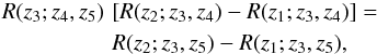$\begin{array}{ccc}\mathit{R}\mathrm{\left(}{\mathit{z}}_{\mathrm{3}}\mathrm{;}{\mathit{z}}_{\mathrm{4}}\mathit{,}{\mathit{z}}_{\mathrm{5}}\mathrm{\right)}& & \left[\mathit{R}\mathrm{\left(}{\mathit{z}}_{\mathrm{2}}\mathrm{;}{\mathit{z}}_{\mathrm{3}}\mathit{,}{\mathit{z}}_{\mathrm{4}}\mathrm{\right)}\mathrm{-}\mathit{R}\mathrm{\left(}{\mathit{z}}_{\mathrm{1}}\mathrm{;}{\mathit{z}}_{\mathrm{3}}\mathit{,}{\mathit{z}}_{\mathrm{4}}\mathrm{\right)}\right]\mathrm{=}\\ & & \end{array}$(17)a relation that just contains the observable shear ratios! Hence, this relation between observables must be obeyed; its violation would indicate a problem with the redshift estimates of the sources and/or lenses. Whereas Eq.(14) probes a combination of the multiplication bias and redshift estimates, Eq.(17) solely probes the latter; in this way, these two effects can be separated.

Curiously, these relations are insensitive to obtaining correct redshifts. For example, Eq.(14) is valid for all z_i, 1 ≤ i ≤ 4. If the sources have a redshift z₄, but in reality are located at redshift ${\mathit{z}}_{\mathrm{4}}^{\mathrm{\prime }}\ne {\mathit{z}}_{\mathrm{4}}$, then the relation (14) still remains true. What is important, however, is that the lens redshift z₂, occurring on the left-hand side, is the same as the source redshift z₂ appearing on the right. We will study in a future work how errors in the mean, the dispersion about the mean, and catastrophic outliers in photometric redshift estimates affect these GSRTs.

5. Discussion

We have derived two relations between measured shear ratios that are independent of the cosmological model, following from two newly derived relations between distances in isotropic spacetimes. The first of these GSRTs, Eq.(14), relates shear ratios to ratios of the multiplicative bias. Hence, if

${\mathrm{ℛ}}_{\mathrm{1234}}\mathrm{\equiv }\mathit{R}\mathrm{\left(}{\mathit{z}}_{\mathrm{2}}\mathrm{;}{\mathit{z}}_{\mathrm{3}}\mathit{,}{\mathit{z}}_{\mathrm{4}}\mathrm{\right)}\left[\mathit{R}\mathrm{\left(}{\mathit{z}}_{\mathrm{1}}\mathrm{;}{\mathit{z}}_{\mathrm{2}}\mathit{,}{\mathit{z}}_{\mathrm{3}}\mathrm{\right)}\mathrm{-}\mathrm{1}\right]\mathrm{-}\mathit{R}\mathrm{\left(}{\mathit{z}}_{\mathrm{1}}\mathrm{;}{\mathit{z}}_{\mathrm{2}}\mathit{,}{\mathit{z}}_{\mathrm{4}}\mathrm{\right)}\mathrm{+}\mathrm{1}$deviates from zero, a redshift-dependent multiplicative bias is a likely origin. Another possible reason for ℛ₁₂₃₄ ≠ 0 could be found in problems with redshift estimates of the source galaxies. The latter is probed by the relation (17), which is independent of the multiplicative bias.

To turn the GSRT into a diagnostic tool for future weak-lensing applications, several aspects need to be studied before. First, the sensitivity for measuring statistically significant deviations of ℛ₁₂₃₄ from zero depends on the number of lenses and sources available for this test, that is, on the sky area of the weak-lensing survey and its depth. It may be conceivable that the lens population is selected based on spectroscopic redshifts. For example, the SDSS has obtained far more than one million spectroscopic galaxy redshifts (Alam et al. 2015), and the upcoming experiments 4MOST (de Jong et al. 2014) and DESI (Flaugher & Bebek 2014) will increase this number by more than an order of magnitude. Alternatively, or in combination, the lens population can be chosen as galaxy clusters, where the upcoming eROSITA X-ray survey mission is expected to detect some 10⁵ clusters (e.g., Pillepich et al. 2012). In a forthcoming paper (Kotula et al., in prep.) we will present a first study of the sensitivity of the GSRT ℛ₁₂₃₄ to variations of M with redshift, including uncertainties in the galaxy redshift distribution that are due to photometric redshifts.

Second, a practical application of the GSRT requires binning of the lens and source samples into redshift bins. Optimal strategies for this binning need to be developed. The estimators will also be affected by the dispersion of the photometric redshift estimates, which needs to be accounted for.

Third, we have assumed an isotropic universe. Our universe is clearly not isotropic on small scales, and hence the Weyl part of the optical tidal matrix in (6) does not vanish. However, the difference between the mean distances in a locally inhomogeneous universe and the distances in the corresponding smooth universe is extremely small (see Schneider et al. 1992, and references therein, as well as the recent detailed discussion by Kaiser & Peacock 2016).

Acknowledgments

I would like to thank Stefan Hilbert, Hendrik Hildebrandt, Jeffrey Kotula, Patrick Simon, and Sandra Unruh for discussions and/or comments on the manuscript. This work was supported by the Transregional Collaborative Research Center TR33 “The Dark Universe” of the German Deutsche Forschungsgemeinschaft, DFG.

References

Appendix A: Validity of Eq.(12) in a Robertson–Walker metric

In this appendix we outline the proof that Eq.(12) holds in a Robertson–Walker metric. This can be shown using the following steps: (i) For the distance ratios β, we can either use the angular-diameter distances, or the comoving angular-diameter distances. Hence,

$\mathit{\beta }\mathrm{\left(}{\mathit{z}}_{\mathit{i}}\mathit{,}{\mathit{z}}_{\mathit{j}}\mathrm{\right)}\mathrm{=}\frac{\mathrm{sn}\mathrm{(}\sqrt{\mathrm{\left|}\mathit{K}\mathrm{\right|}}\hspace{0.17em}\mathrm{[}{\mathit{\chi }}_{\mathit{j}}\mathrm{-}{\mathit{\chi }}_{\mathit{i}}{\mathrm{\left]}}^{\mathrm{\right)}}}{\mathrm{sn}\mathrm{(}\sqrt{\mathrm{\left|}\mathit{K}\mathrm{\right|}}\hspace{0.17em}{\mathit{\chi }}_{\mathit{j}}\mathrm{)}}\mathrm{=}\frac{\mathrm{sn}\mathrm{(}{\mathit{x}}_{\mathit{j}}\mathrm{-}{\mathit{x}}_{\mathit{i}}\mathrm{)}}{\mathrm{sn}\mathrm{\left(}{\mathit{x}}_{\mathit{j}}\mathrm{\right)}}\mathit{,}$where the function sn(x) is either the sine or the hyperbolic sine, depending on the sign of the curvature parameter K, and in the limiting case of K = 0, it is the identity. Furthermore, χ_j is the comoving distance to redshift z_j, and we defined ${\mathit{x}}_{\mathit{j}}\mathrm{=}\sqrt{\mathrm{\left|}\mathit{K}\mathrm{\right|}}{\mathit{\chi }}_{\mathit{j}}$. (ii) Using the above expression, we can write Eq.(12) after multiplication by sn(x_k) sn(x_l) as 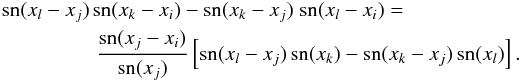$\begin{array}{ccc}\mathrm{sn}\mathrm{(}{\mathit{x}}_{\mathit{l}}\mathrm{-}{\mathit{x}}_{\mathit{j}}\mathrm{)}& & \mathrm{sn}\mathrm{(}{\mathit{x}}_{\mathit{k}}\mathrm{-}{\mathit{x}}_{\mathit{i}}\mathrm{)}\mathrm{-}\mathrm{sn}\mathrm{(}{\mathit{x}}_{\mathit{k}}\mathrm{-}{\mathit{x}}_{\mathit{j}}\mathrm{)}\mathrm{sn}\mathrm{(}{\mathit{x}}_{\mathit{l}}\mathrm{-}{\mathit{x}}_{\mathit{i}}\mathrm{)}\mathrm{=}\\ & & \frac{\mathrm{sn}\mathrm{(}{\mathit{x}}_{\mathit{j}}\mathrm{-}{\mathit{x}}_{\mathit{i}}\mathrm{)}}{\mathrm{sn}\mathrm{\left(}{\mathit{x}}_{\mathit{j}}\mathrm{\right)}}\mathrm{[}\mathrm{sn}\mathrm{(}{\mathit{x}}_{\mathit{l}}\mathrm{-}{\mathit{x}}_{\mathit{j}}\mathrm{)}\hspace{0.17em}\mathrm{sn}\mathrm{\left(}{\mathit{x}}_{\mathit{k}}\mathrm{\right)}\mathrm{-}\mathrm{sn}\mathrm{(}{\mathit{x}}_{\mathit{k}}\mathrm{-}{\mathit{x}}_{\mathit{j}}\mathrm{)}\hspace{0.17em}\mathrm{sn}\mathrm{(}{\mathit{x}}_{\mathit{l}}{\mathrm{)}}^{\mathrm{]}}\mathit{.}\end{array}$(iii) Next we make use of the addition theorem, sn(a−b) = sn(a) cn(b)−cn(a) sn(b), where cn(x) is either cos(x), cosh(x), or ≡ 1, depending on K. After applying the addition theorem to the foregoing equation, a term-by-term comparison of both sides shows its validity.

References

- Alam, S., Albareti, F. D., Allen de Prieto, C., et al. 2015, ApJS, 219, 12 [NASA ADS] [CrossRef] [Google Scholar]
- Bartelmann, M., & Schneider, P. 2001, Phys. Rep., 340, 291 [NASA ADS] [CrossRef] [Google Scholar]
- Bartelmann, M., Viola, M., Melchior, P., & Schäfer, B. M. 2012, A&A, 547, A98 [NASA ADS] [CrossRef] [EDP Sciences] [Google Scholar]
- Bernstein, G. M. 2010, MNRAS, 406, 2793 [NASA ADS] [CrossRef] [Google Scholar]
- Bernstein, G. M., & Armstrong, R. 2014, MNRAS, 438, 1880 [NASA ADS] [CrossRef] [Google Scholar]
- Das, S., Errard, J., & Spergel, D. 2013, ArXiv e-prints [arXiv:1311.2338] [Google Scholar]
- de Jong, R. S., Barden, S., Bellido-Tirado, O., et al. 2014, in Ground-based and Airborne Instrumentation for Astronomy V, Proc. SPIE, 9147, 91470M [Google Scholar]
- Flaugher, B., & Bebek, C. 2014, in Ground-based and Airborne Instrumentation for Astronomy V, Proc. SPIE, 9147, 91470S [NASA ADS] [CrossRef] [Google Scholar]
- Heymans, C., Van Waerbeke, L., Bacon, D., et al. 2006, MNRAS, 368, 1323 [NASA ADS] [CrossRef] [Google Scholar]
- Jain, B., & Taylor, A. 2003, Phys. Rev. Lett., 91, 141302 [NASA ADS] [CrossRef] [PubMed] [Google Scholar]
- Kaiser, N., & Peacock, J. A. 2016, MNRAS, 455, 4518 [NASA ADS] [CrossRef] [Google Scholar]
- Kilbinger, M. 2015, Rep. Progr. Phys., 78, 086901 [NASA ADS] [CrossRef] [Google Scholar]
- Kitching, T. D., Viola, M., Hildebrandt, H., et al. 2016, MNRAS, submitted [arXiv:1512.03627] [Google Scholar]
- Mandelbaum, R., Rowe, B., Armstrong, R., et al. 2015, MNRAS, 450, 2963 [NASA ADS] [CrossRef] [Google Scholar]
- Massey, R., Heymans, C., Bergé, J., et al. 2007, MNRAS, 376, 13 [NASA ADS] [CrossRef] [Google Scholar]
- Melchior, P., & Viola, M. 2012, MNRAS, 424, 2757 [NASA ADS] [CrossRef] [Google Scholar]
- Miller, L., Heymans, C., Kitching, T. D., et al. 2013, MNRAS, 429, 2858 [Google Scholar]
- Pillepich, A., Porciani, C., & Reiprich, T. H. 2012, MNRAS, 422, 44 [NASA ADS] [CrossRef] [Google Scholar]
- Rozo, E., & Schmidt, F. 2010, ArXiv e-prints [arXiv:1009.5735] [Google Scholar]
- Schneider, M. D., Hogg, D. W., Marshall, P. J., et al. 2015, ApJ, 807, 87 [NASA ADS] [CrossRef] [Google Scholar]
- Schneider, P. 2016, A&A, submitted [arXiv:1409.0015] [Google Scholar]
- Schneider, P., Ehlers, J., & Falco, E. E. 1992, Gravitational Lenses, (New York: Springer-Verlag Heidelberg), 112 [Google Scholar]
- Seitz, C., & Schneider, P. 1997, A&A, 318, 687 [NASA ADS] [Google Scholar]
- Seitz, S., Schneider, P., & Ehlers, J. 1994, Class. Quant. Grav., 11, 2345 [Google Scholar]
- Taylor, A. N., Kitching, T. D., Bacon, D. J., & Heavens, A. F. 2007, MNRAS, 374, 1377 [NASA ADS] [CrossRef] [Google Scholar]
- Voigt, L. M., & Bridle, S. L. 2010, MNRAS, 404, 458 [NASA ADS] [Google Scholar]