| Issue |
A&A
Volume 592, August 2016
|
|
|---|---|---|
| Article Number | A39 | |
| Number of page(s) | 8 | |
| Section | Planets and planetary systems | |
| DOI | https://doi.org/10.1051/0004-6361/201628298 | |
| Published online | 18 July 2016 | |
Effects of disc asymmetries on astrometric measurements
Can they mimic planets?
1 Institute of Astronomy, University of Cambridge, Madingley Road, Cambridge CB3 0HA, UK
e-mail: qkral@ast.cam.ac.uk
2 Observatoire de Paris, LUTh-CNRS, UMR 8102, 92190 Meudon, France
e-mail: jean.schneider@obspm.fr
3 NaXys, University of Namur, Rempart de la Vierge 8, 5000 Namur, Belgium
Received: 12 February 2016
Accepted: 20 May 2016
Astrometry covers a parameter space that cannot be reached by RV or transit methods to detect terrestrial planets on wide orbits. In addition, high accuracy astrometric measurements are necessary to measure the inclination of the planet’s orbits. Here we investigate the principles of an artefact of the astrometric approach, namely the displacement of the photo-centre owing to inhomogeneities in a dust disc around the parent star. Indeed, theory and observations show that circumstellar discs can present strong asymmetries. We model the pseudo-astrometric signal caused by these inhomogeneities, asking whether a dust clump in a disc can mimic the astrometric signal of an Earth-like planet. We show that these inhomogeneities cannot be neglected when using astrometry to find terrestrial planets. We provide the parameter space for which these inhomogeneities can affect the astrometric signals but still not be detected by mid-IR observations. We find that a small cross section of dust corresponding to a cometary mass object is enough to mimic the astrometric signal of an Earth-like planet. Astrometric observations of protoplanetary discs to search for planets can also be affected by the presence of inhomogeneities. Some further tests are given to confirm whether an observation is a real astrometric signal from a planet or an impostor. Eventually, we also study the case where the cross-section of dust is high enough to provide a detectable IR-excess and to have a measurable photometric displacement by actual instruments such as Gaia, IRAC, or GRAVITY. We suggest a new method, which consists of using astrometry to quantify asymmetries (clumpiness) in inner debris discs that cannot be otherwise resolved.
Key words: astrometry / circumstellar matter / protoplanetary disks
© ESO, 2016
1. Introduction
The search for and observation of exoplanets is growing in three directions: new detection techniques are still emerging, ever more planets being discovered and more data being collected on each planet. The detection techniques each have their specificities regarding the accessible planet observables. Among them, astrometry is still in its infancy since, as of January 2016, only a handful of astrometric detections of exoplanet candidates have been announced, namely DE0823-49 b (Sahlmann et al. 2015) and HD 176051 b (Muterspaugh et al. 2010). Another candidate, VB 10 b, claimed to be detected by astrometry (Pravdo & Shaklan 2009), has been challenged by Bean et al. (2010) and by Anglada-Escudé et al. (2010). We shall present a plausible reason that reconciles the three studies in the discussion. This technique still has a promising capability, which is to detect low-mass planets, determine the geometry of their orbits and, more importantly, measure their masses.
Just like any technique, astrometry has its own source of noise and artefacts. Until now, the only noise source limiting the sensitivity to low masses that was investigated is the activity of the central star. The latter indeed introduces a fluctuation of the centroid of the star position (Lagrange et al. 2011).
Here we investigate an artefact of the astrometric approach, first emphasised by Schneider (2011), whose preliminary results show that an astrometric signal subject to a perturbation by an axially asymmetric dust disc can mimic the dynamical effect of planetary companions.
This study is important in the context of astrometric projects aiming at the detection of Earth-like planets in the habitable zone of nearby stars (e.g. NEAT, Malbet et al. 2012). On the ground, the GRAVITY (Lacour et al. 2014) and SKA (Fomalont & Reid 2004) instruments or projects have an astrometric accuracy of a few microarcsec. For Earth-like planets, the astrometric signal expected is on the order of 0.3 μas around a sun-like star at 10 pc (see Eq. (2)) and artefacts of this order of magnitude could mimic these planets. Therefore these artefacts have to be taken into account.
We first present the general mathematical formalism in Sect. 2 and show how it works in a range of cases in Sect. 3. In Sect. 4, we provide tests to discriminate a disc-induced artefact from a real stellar wobble. Finally, we compare the effect of inhomogeneities to the performance of present and future astrometric instruments such as Gaia (de Bruijne 2012), GRAVITY, TMT (Sanders 2013) and NEAT. Furthermore, we discuss a new interesting detection technique to observe clumpiness in discs.
2. Impact of inhomogeneities on parent star astrometry
In this section we consider the case of stellar light reflected by some dust inhomogeneities, as well as its thermal emission. The point of using astrometry is to reach accuracy below the resolution of the system. In this study, we are thus interested in inhomogeneities that cannot be resolved. For this reason, the dust creating these inhomogeneities must be close to its host star. For an observation at a wavelength λ with a telescope of diameter d, the typical spatial resolution is λ/d meaning that for NEAT in the optical, the resolution is ~0.1 arcsec. As a result, inhomogeneties that would affect astrometric measurements without being resolved will be within 0.1′′, i.e. within 1 au (10 au) for a system at 10 pc (100 pc).
The brightness distribution of inhomogeneities is a function of time since the disc structure evolves essentially according to its Keplerian motion. Thus, the difference in position between the star and the displacement owing to the presence of an asymmetric disc can be given as a function of the inhomogeneity to star flux ratio Iinh/I⋆. If a companion is present, it also changes the observed position of the star and this is what is used to detect planets with astrometric measurements.
As astrometry is performed below the resolution limit, we observe the displacement of the photo-centre of the system. The global photo-centre displacement Δα is a superposition of the barycentric dynamical astrometric displacement ΔαB and the photo-centric displacement Δαph due to the asymmetric brightness distribution of the unresolved disc (see Fig. 1).
If αph is the angular separation of the photo-centre of an inhomogeneity in the disc, of brightness ratio Iinh/I⋆, with respect to the parent star, then the star+inhomogeneity photo-centre position has an angular offset Δαph with respect to the parent star’s centroid given by 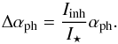 (1)By definition, neglecting the mass of the disc inhomogeneities, the barycentric displacement that is due to a companion with mass MC gives
 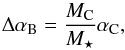 (2)where αC = a/D is the angular separation of the companion, a is the barycentre-planet distance projected on the sky at the measurement epoch, and D the distance of the star to the observer.
If we now assume that the photo-centre displacement is created by an inhomogeneity at distance a so that αph = a/D and the amplitude of the displacement Δα = Iinh/I⋆(a/D), where a is in au, D in pc and Δα in arcsec.
First, we plot in Fig. 2Iinh/I⋆ as a function of a assuming a distance D = 10 pc, for different values of Δα (black solid lines). As given by Eq. (1), when Iinh/I⋆ increases, for a given a/D, Δα increases. Also, for a given Δα, Iinh/I⋆ ∝ 1 /a. The location of an Earth-like planet in terms of its Δα needed at 1au to mimic an Earth is shown as a red square in Fig. 2. This gives the inhomogeneity-to-star flux ratio required to mimic an Earth. On the right plot, this location changes as the host star is more massive by a factor ~1.8. Indeed, using Eq. (2), we can rewrite it in these more useful terms: 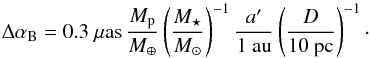 (3)Simply assuming that habitable planets around more or less luminous stars reside at distances where the insolation is equal to the Earth’s, then a′ = a (L⋆/L⊙)0.5 is the new location of the planet. The location of an Earth-like planet around β Pic is then at a′ = 2.83 au and would imply a displacement of 0.47 μas.
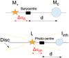 |
Fig. 1 Top: schematic of the usual barycentric photo-centre displacement ΔαB used in astrometry to detect a planet of mass MC at distance a from the barycentre with the star of mass M⋆. Bottom: the photo-centre displacement Δαph is now caused by an inhomogeneity of flux Iinh at distance a orbiting around a star of flux I⋆ and possibly surrounded by a disc shown with yellow lines. |
We assess the detectability of such inhomogeneities using the WISE detection limits at λlim = 12 μm. At a given astrometric observing wavelength λinh, we compute the minimum value of Iinh/I⋆ that could be detected by WISE at different a. To do so, we assume that the detections are limited by our ability to differentiate the WISE photometry from the stellar flux (or “calibration limited”) and that the grains behave like pseudo-black bodies with an albedo ω = 0.2. We find that, in thermal emission, the minimum detected flux ratio at wavelength λinh is given by 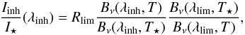 (4)where Bν is the Planck function and Rlim is the WISE calibration limit (~10%). To get this formula, we compute the disc-to-star flux ratio at a certain wavelength λlim set by the WISE sensitivity and shift it to another (thermal) wavelength λinh where the astrometry is done. The albedo does not appear in this equation since it affects both the WISE and the astrometric wavelengths equally. Similarly, in scattered light, converting the thermal detection limit to an optical flux, this limit is defined by
 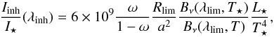 (5)where L⋆ is the star’s luminosity in solar luminosity, T⋆ the star’s temperature (in K), and a is in au.
  is the black body temperature of the inhomogeneity. We assumed that the absorption/scattering properties are wavelength independent (i.e. albedo is monochromatic), but we illustrate what happens in Fig. 3 for a full Mie calculation.
 |
Fig. 2 Left: Iinh/I⋆ as a function of the distance to the star a (in au) for different photo-centre displacements (Δα = [ 0.01,1,100 ] μas) in black solid lines. WISE (12 μm) detection limit in terms of Iinh/I⋆ are shown in red for a dust cloud orbiting at a around a sun-like star and observed at different wavelengths representing different potential instruments, 0.55 (solid, Gaia or NEAT), 2.2 (dotted, GRAVITY) and 20 (dashed, TMT) microns. The position of an Earth-like planet is represented with a red square. Right: Same for a dust cloud orbiting a β-Pic like A6V star. In this case, the Earth-like planet having the same irradiation and mass as Earth, is located at 2.83 au (see text for details). |
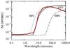 |
Fig. 3 Photo-centre displacement as a function of wavelength for a Keplerian dust cloud orbiting at 1au around a G2V star at 10 pc (solid lines). The thicker of the G2V lines is the numerical model. We also vary the spectral type of the host star using the analytical model. The dotted line is for an A6V star and the dashed line for an M8V star. |
The red curves in Fig. 2 show the corresponding limits for different observing wavelengths λinh equal to 0.55 (solid line, for Gaia, NEAT), 2.2 (dotted line, for GRAVITY) and 20 (dashed line, for TMT) μm. The left plot is for the case of a sun-like star and the right plot for a β Pic-like star. In the latter case, we consider an Earth-like planet as having the same irradiation and mass as Earth, so it is located at 2.83 au as stated earlier when defining a′. Above each red line, the dust inhomogeneity could be detected by WISE at 12 μm. We note the wide range of the parameter space where some dust could be undetected but still create a photo-centre displacement big enough to mimic an Earth-like planet. The limits on the amount of dust depend on the type of host star (which changes the dust temperature) as well as λinh. For observations of the astrometric displacement in the optical, the emission is dominated by scattered light whilst, at 20 μm, only thermal emission is present. For the λinh = 2.2 microns case shown in the plot, both thermal emission and scattered light can be significant depending on the distance to the star, which explains the two regimes observed on the dotted line. Indeed, for a sun-like (β Pic like) star, within 0.2 au (0.8 au), the grains are so hot that thermal emission becomes dominant over scattered light. We conclude here that there is still a large parameter space (which gets larger for lower mass stars) where inhomogeneities can be bright enough to induce a photo-centre displacement but still be undetectable. Of course, the detection of an IR-excess in a system with an astrometric detection does not guarantee that the dust is the cause, since the dust distribution could be axisymmetric.
3. Various cases of inhomogeneities in planetary systems
3.1. Overview of the different cases
The inhomogeneities presented in the previous section can be classified in two different categories of axial asymmetries in discs: static and non static. Beyond that general dichotomy, it is not trivial to describe the diversity of asymmetric morphologies by a limited number of categories. One could imagine diverse situations such as so-called bright spots, vortices, spiral structures or even giant impacts. The static inhomogeneities lead to a photo-centre displacement that is constant in time and can therefore not mimic the stellar motion as a result of a companion. Thus, the only inhomogeneities that we are interested in are non-static configurations. For this reason, we discard giant impacts, which show a strong asymmetry at the collision point at steady state but which does not move, and could be distinguished from a planet (Kral et al. 2015). For the same reasons, the warps in discs (created by an inclined planet) and pericentre glow effects (brightness asymmetry owing to secular perturbations by an eccentric planet, leading to an eccentric disc) are discarded. The interesting cases that could affect astrometric measurements can be summed up as follows:
-
(1) Bright spots (dust cloud in a disc, clumps owing to a resonancewith a planet);
-
(2) Spiral structures (owing to a planetary companion or a fly-by with a nearby star);
-
(3) Inhomogeneities in protoplanetary discs (vortices, planet induced spirals, etc.);
-
(4) Non static others.
Let us now parametrise the different non-static configurations listed above relaxing the previous black-body assumption and assess their respective impacts on astrometric observations.
-
Bright spots Bright spots are observed in discs and are expected in theory. These bright spots could be dust clouds that are created by dust produced in collisions between planetesimals within an otherwise undetectable debris disc (Wyatt & Dent 2002; Zeegers et al. 2014). One could also imagine that the spots are dust clumps that stay within the Hill sphere of planetesimals. These enshrouded planetesimals are surrounded by a swarm of irregular satellites that collide and create the dust cloud (Kennedy & Wyatt 2011). Another possibility would be that planetesimals are surrounded by rings, such as the centaur Chariklo (Braga-Ribas et al. 2014), but more massive and with a high albedo. These clumps are also expected to trail behind planets, as in the Earth’s resonant ring that co-rotates with Earth (Wyatt et al. 1999). More generally, dust grains can be trapped in mean-motion resonances with planets when migrating inwards because of Poynting-Robertson drag, which can create luminous dust clumps (e.g. Shannon et al. 2015). We do not intend to be exhaustive here, but rather give an idea of several configurations that could create these bright spots. In this case, we can use Eq. (1), where Iinh = Ispot(as,λ), the spot flux at wavelength λ and, at a projected distance, as that we shall assume to be the semi-major axis of the dust cloud for simplicity. Also, αph = as/D, where D is the distance to Earth. Ispot is the sum of thermal emission Ispotth and scattered light Ispotsca. Ispotth (assuming a fixed composition) is equal to
 (6)where σabs is the absorption/emission cross section of the cloud for a given grain size s, i.e. 4πs2Qabs(s,λ) and Bν(Ts) is the Planck function for a temperature Ts. Qabs is the dimensionless absorption/emission coefficient, which for a given grain size depends only on the wavelength λ. dN(s) ∝ s− q ds is the size distribution of grains. We choose the standard q = 3.5 value to model dust clouds (e.g. Kral et al. 2013). The grain temperature Ts is worked out solving the thermal equilibrium of grains using the code GRaTeR (Augereau et al. 1999; Lebreton et al. 2013). Indeed, for small grains the black-body assumption is far from being accurate and, since we are interested in the whole wavelength range for astrometric measurements, we assess the infrared emission from the dust properly through Eq. (6). Similarly, for the case of scattered light
  (7)where
  , Qsca being the dimensionless scattering coefficient, and f(φ) is the phase function, which is equal to 1/4π since we assume isotropic scattering.
 -
Spiral structures Two types of spiral structures can develop in debris discs. Spirals that are due to tidal forces, following the passage of, for instance, an unbound companion or, over longer timescales, as a result of differential precession in the case of a bound companion. The tidally induced spiral evolves quickly since its evolution is set up by the differential rotation of the disc dΩ/dR, where Ω is the orbital frequency and R the distance of planetesimals. The probability of witnessing these spirals is thus rather low and we do not intend to model them. For the other type of spiral, the evolution is set by the differential precession of the orbits dωp/ dR, where ωp is the precession velocity of the orbits. We find that, for a circular perturber of mass Mp and semi-major axis ap (Augereau & Papaloizou 2004),
 (8)The evolution of these types of spirals is then very slow compared to the Keplerian evolution and could not be misinterpreted as being a planet.
 -
Inhomogeneties in protoplanetary discWe created a general category for these young systems that are still surrounded by a protoplanetary disc and we give some specific cases that could interfere with astrometric measurements. We expect vortices to be present in protoplanetary discs that are induced either by the Rossby-wave instabilities (RWI, Lovelace et al. 1999) or baroclinic instabilities (Lesur & Papaloizou 2010). In the case of the RWI, this can be triggered either on the edge of a gap carved out by giant planets or at the interface with dead zones. These vortices can even be created very close to the star at the inner disc edge at the boundaries between turbulent, magnetised, and accreting regions (Faure et al. 2015; Ansdell et al. 2016). These vortices can survive for several orbits, which can be shortened depending on several complicated effects such as, for instance, the amount of turbulence or dust feedback effects (Fu et al. 2014). One such vortex was plausibly observed by ALMA (Van der Marel et al. 2013). These vortices can be, as a first approximation, modelled as we have done for dust clouds. As large dust concentrates in the vortex centre, we take a shallower size distribution within the affected size range as explained in Lyra & Lin (2013). Planet-induced spirals (Tanaka et al. 2002) are expected in protoplanetary discs and both the contribution of the planet and the spirals could end up in the astrometric measurements. Gravitational instabilities may develop in protoplanetary discs and lead to fragmentation and clump formation (e.g. Meru 2015). SAO 206462 is an example of a young disc presenting spiral features that could be generated with either a planet or gravitational instability (Garufi et al. 2013). Spiral waves may also be triggered by shadows in transition discs (Montesinos et al. 2016), or even by an inflow coming from the residual external envelope of protoplanetary discs (Lesur et al. 2015). We also note that mid-IR variability has been observed in many protoplanetary discs (Flaherty et al. 2014). This may be due to variations in the structure of the inner rim of the protoplanetary disc. Depending on the disc orientation, this would also cause an astrometric effect. The astrometric displacement derived from this type of a variation would also depend on the inclination and might not look like an ellipse, however, since the bright spot (e.g. the puffed up bit of the rim) would not necessarily be visible for the whole orbit.
-
Others This subsection includes the case of many different substructures that can be found in planetary systems that shall be treated on a case-by-case basis. For example, the case of AU Mic shows that we do not yet fully understand all types of inhomogeneities (Boccaletti et al. 2015). In this system, some dust clumps are observed as moving radially outwards with time. It can be modelled as a dust clump that is composed of unbound grains and is moving radially outwards.
3.2. Quantifying the effect of inhomogeneities for some specific cases of debris and protoplanetary discs
We now evaluate the quantitative effect of disc asymmetries listed in Sect. 3.1. Since we have in mind astrometric programs with timescales of less than 10 yr, we must consider the inner part of discs that are closer than 1 arcsec to the parent star. These regions have not yet been investigated, with the exception of a few interferometric observations (e.g. Fomalhaut, Lebreton et al. 2013) and photometric light curves (Rodriguez et al. 2016). We are thus constrained to rely on models by extrapolating below 1 arcsec (assuming systems close to the Earth) observations that are made further than 1 arcsec from the parent star.
-
Bright spots For this example, we model a dust cloud orbiting at 1au around a sun-like star at 10 pc. We would like to check that Fig. 2 still holds when relaxing the black-body assumption. A signal that could mistaken for an Earth-like planet, with the same orbital period and the same astrometric amplitude, would create a 0.3 μas astrometric signal. This converts to Iinh/I⋆ = 3 × 10⁻⁶ or a total cross-section of σtot ~ 1018 m2. Thus, we input a dust cloud with a cross section of 1018 m2. The minimum grain size in the dust cloud is set by a radiation pressure cut-off, which is ~1 micron for this type of host star. We fix the maximum size as being 100 m, but we note that the biggest bodies do not contribute to the flux at all. This fixes the total mass as 3 × 10¹⁹ kg (30 times lighter than Ceres). We use a conventional size distribution with q = 3.5. The photometric displacement, which is due to the dust cloud, depends on the wavelength as shown in Fig. 3. It creates a Δα = 0.4 μas in the optical, which is close to the expected 0.3 μas in the optical. For longer wavelength, the astrometric displacement is even larger. We overplot the results of our analytical model for varying spectral types (A6V, G2V, and M8V) in Fig. 3. The values predicted with our black-body assumption provide a very good estimate of the real displacement. However, we note two major differences: First, by comparing the numerical model (thick line) and the analytical black-body assumption, we notice that they behave differently at longer wavelengths because grains are inefficient emitters when λ>s. Secondly, the break between the scattered light-dominated regime (smaller λ) and the thermal emission dominated regime happens at longer λ for later spectral types (see Sect. 4.3 for more details). This implies that an undetectable cometary mass body, if broken up and distributed as a collisional cascade-size distribution, is enough to create a signal greater than 0.3 μas (which is the astrometric displacement owing to an Earth-like planet at 1 au at 10 pc) in the optical. This dust cloud is then able to mimic an Earth-like planet as could any more massive dust clouds as well. The mass is too small to change the barycentre position significantly so that the only contribution to the photo-centre displacement is from the dust cloud brightness.
-
Inhomogeneities in protoplanetary discs Most of the inhomogeneities presented in Sect. 3.1 for protoplanetary discs could be modelled with a bright spot. For instance, vortices could easily be modelled with a dust cloud with two different size distributions since the biggest grains, with a Stokes number close to one, are most easily trapped. We emphasise however that these features are surrounded by protoplanetary discs that should definitely be detected if present (e.g. by IR-excess). Anyway, all the cases presented in Sect. 3.1 might arise, but since most of them can be modelled with a bright spot, a more refined study is left for the future when astrometric data of systems hosting a protoplanetary discs will be available. We use Fig. 2 (right) to see that Iinh/I⋆ needs to be ~1.5 × 10⁻⁶ to mimic an Earth-like planet around an A6V star (a′ = 2.83 au) at 10 pc, which translates as a total cross-section equal to 2 × 10¹⁸ m2. Using this cross-section, we check with GRaTeR that the results are very similar to those presented in Fig. 3. This cross-section is sufficient to imply a displacement of the photo-centre that is large enough to perturb the detection of an Earth-like planet. This confirms once again that our black-body approximation in Fig. 2 provides reliable results. Indeed, the photo-centre displacement created by the inhomogeneity emission is equal to the expected 0.45 μas (see Eq. (3)) in the optical and is greater at longer wavelength, as is found for the bright spot case (see Fig. 3). The displacement induced at longer wavelengths could be detected by high accuracy astrometric instruments such as SKA or even using IRAC/Spitzer, which can reach an astrometric precision of ~20 mas (Esplin & Luhman 2016). This shows that astrometric observations of systems hosting protoplanetary discs may be affected by these asymmetric structures. Disentangling a real planet from these inhomogeneties requires extra work as explained in details in Sect. 4.
-
Others As an example of so-called other configurations, we take the disc around AU Mic. This shows fast, apparently non-Keplerian, motions of spots. Assuming a contrast ratio of 10-5 relative to the parent star corresponding to the high-contrast imaging performances of the images of AU Mic with SPHERE (see Boccaletti et al. 2015), the features A, B, C, D, and E lead to the pseudo-astrometric effects listed in Table 1 (derived from their Fig. 3b) at epochs 2011 (HST) and 2014 (SPHERE).
Table 1Pseudo-astrometric effects (in μas) implied by the different features A, B, C, D, E recently discovered in AU Mic (see text for details).
Assuming an astrometric instrument with a 1 arcsec resolution, only the spine A would have an astrometric effect on the parent star. This would lead to an astrometric difference between 2011 and 2014 of 2 μas. This corresponds to an astrometric effect that is linear in time between 2011 to 2014; it can therefore not mimic the Keplerian motion of a companion with a period of only a few years, since the transverse velocity of the latter would be sinusoidal on an edge-on orbit.
4. Tests to confirm an astrometric planet detection
Here we discuss some observational tests to check if an apparent photo-centre displacement is due to a barycentric effect by a companion or to a disc asymmetry.
4.1. Comparison with radial velocity measurements
Some bright non-static asymmetries could mimic a pseudo-planet sufficiently massive to be detectable by radial velocity measurements. A first basic check would therefore consist of monitoring the radial velocity of the parent star, if permitted by the stellar spectrum.
The proposed test has been applied by Anglada-Escudé et al. (2010) and by Bean et al. (2010) to the planet candidate claimed by Pravdo & Shaklan (2009) to be detected by astrometry. These authors did not detect it by radial velocity, concluding that VB 10 b does not exist. We suggest that a possible explanation of the contradiction between the astrometric claim by Pravdo & Shaklan and the negative result from radial velocities measurement consists of an astrometric effect that is due to an asymmetric disc inhomogeneity. We recomputed Fig. 2 for this case, where the host star has very low luminosity (M8V star) and temperature (~2700 K). The detection limit given by WISE for this case is very high, which would permit a massive dust cloud that creates a Δαph greater than 1mas to be present without being detectable.
4.2. Time evolution
If the photo-centre evolution is a stellar wobble owing to a companion, it must correspond to a Keplerian motion. These Keplerian motions are also created by bright spots and vortices, while the cases of AU Mic or spiral evolution show that, in some instances, the effective photo-centre displacement may be non-Keplerian. A first test is thus to check if the displacement is Keplerian. If not, the wobble is not due to a companion.
However, it is not as straightforward if there is more than one planetary companion with different periods, since the stellar wobble is then different from a simple Keplerian motion. Conversely, if the displacement is Keplerian, it is not proof that it is a dynamical stellar wobble as explained in this paper. The eccentricity of the object creating the astrometric signal may give some clues as to the favoured scenario: planet versus dust. Indeed, dust clouds could be expected to have a rather low eccentricity but planets can reach higher values. This cannot be claimed to be a reliable test, but gives some hints on how to disentangle the different possibilities.
4.3. Chromaticity
The dynamical stellar wobble induced by one (or more) companion is wavelength independent. In particular this must be the same in reflected light (in the visible and near-infrared domain) and in the thermal regime (mid-infrared to mm). An achromaticity1 of the photo-centre displacement is a strong test of its purely dynamical origin. Conversely, an inhomogeneity would create a chromatic signal (e.g. see Fig. 3). Therefore, whenever possible, a candidate astrometric displacement should be observed in at least two wavelength regimes where a change is expected. The two observing wavelengths must be chosen according to the spectral type of the host star as the break between a reflected light-dominated regime and a thermal emission regime happens at longer wavelengths for later spectral types (see Fig. 3). For M dwarfs, we need to look in the far-IR to mm to see a difference, whereas for an early A-type star, NIR or mid-IR observations will already show a difference. In any case, observing at longer wavelengths seems more favourable and SKA should be a good instrument to achieve these observations.
In the above subsection, looking at comparisons with radial velocity measurements we have suggested that the pseudo-astrometric detection of VB 10 b is due to an asymmetric disc inhomogeneity. One way to explain this would be to show that the detection of the astrometric effect detected by Pravdo & Shaklan at 550–750 nm is wavelength dependent, for instance, in the far-IR or submillimetric regimes. We recommend observing it with SKA, when built, using astrometry or the Large Binocular Telescope Interferometer (LBTI, Defrère et al. 2016) to look for warm dust.
4.4. Direct imaging
Direct imaging can be used a posteriori for a confirmation or rejection of the candidate astrometric signal. Indeed, a very strong test would consist in a high angular resolution image of the stellar environment to investigate possible non-static asymmetries in a disc. In addtion, this is a good way to disentangle an astrometric signal coming from both an inhomogeneity and a planet (the achromoticity vs chromaticity of the signal could also be used), as would be created by an equivalent to the Earth’s resonant ring that corotates with Earth (Wyatt et al. 1999). In the visible and near-infrared, the GPI camera on the Magellan telescope and the SPHERE camera on the VLT (and in the millimetric regime the ALMA instruments) are well adapted to this task. However, direct imaging of discs is only possible for the brightest systems with a fractional luminosity greater than about 10-4 and so far there are no cases where a disc has been imaged but no IR-excess has been detected. As for protoplanetary discs, seeing structures within a few au is not yet possible for the distances they reside in. Therefore, direct imaging could only be useful for detecting the supposed planet that has otherwise been detected by astrometry.
5. Discussion
We note that a byproduct of our discussion of the wavelength dependence of a pseudo-astrometric effect is to suggest detecting astrometrically inner discs that are not detectable by imaging and to constrain their asymmetry. It could in particular first be applied to some systems where falling evaporating bodies (FEBs) are known, such as β Pictoris or HD 172555 (Beust et al. 1998; Kiefer et al. 2014). It could also be tried on systems where interferometric observations seem to show the presence of hot dust called exozodis (Absil et al. 2013; Ertel et al. 2015). The final aim would be to apply this astrometric method to randomly probe the inner parts of planetary systems and discover hidden components, such as FEBs, asymmetric exozodis, or even trailing clumps behind planets, such as the Earth’s resonant ring that corotates with Earth (Wyatt et al. 1999).
Thus, while we have shown that unseen dust in the inner regions of planetary systems may masquerade as planets, the same technique could be used to probe the structure of known warm dust populations. For example, the ~1 Gyr old star η Corvi hosts both warm and cool dust components (Wyatt et al. 2005), with the warm component residing at about 1au (Smith et al. 2009; Defrère et al. 2015). The origin of the warm component is unknown, but is thought to be the outcome of a system-wide recent or ongoing dynamical instability (Lisse et al. 2011). Recent observations with the LBTI constrained this dust to lie within a projected distance of 1au (Defrère et al. 2015), less than the 3 au predicted by modelling of the infrared spectrum (Lisse et al. 2011), with one possible resolution being that the warm dust component is clumpy. The disc-to-star flux ratio at 12 μm is 1.2, roughly two times higher than the detectable limit. Thus, assuming a Solar mass star, the curved lines in the left panel of Fig. 1 show the level of astrometric signal that would result if 50% of the warm component were concentrated in a single clump near 1au (though overestimated by a factor of two, since η Corvi is 18 pc distant). The astrometric signal would be a few micro-arcseconds for an optical mission, and around 10 mas for mid-IR observations. GRAVITY astrometric precision is on the order of a few μas and could detect this type of star’s displacement (Lacour et al. 2014). In the mid-IR, the astrometric capabilities of IRAC/Spitzer of ~20 mas could be used to probe these azimuthal structures at longer wavelengths (Esplin & Luhman 2016). Thus, high precision astrometry provides a possible way to probe the azimuthal structure of warm dust.
The detection limits that were used in Fig. 2 were photometric, but for specific systems it is possible to go deeper. Indeed, it might be possible to rule out a dust spot scenario using nulling interferometry (LBTI), which can go a few orders of magnitude deeper (Defrère et al. 2016). However, LBTI requires bright stars, so this option would only be available for the nearest stars, which is the most interesting since this is where astrometric measurements are most sensitive.
Gaia is going to detect at least 20 000 Jupiter-mass planets or larger (Perryman et al. 2014). The astrometric effect of these planets is quite large (>100 μas according to Eq. (3)) and for most stellar types it would mean that, if dust was mimicking these planets, it would be detectable. It is clearly shown in Fig. 2, where a Jupiter-like planet with Δα = 100 μas lies above the sensitivity line when observed in the optical. We note that there are more bands than WISE 12 μm and they could also be used. Hence, a lack of an IR-excess rules out the possibility that an astrometric detection is dust but an IR-excess does not mean the planet is not real, since the dust could be axisymmetric.
Another source of perturbation is the transit of a planet. Indeed, from the ingress to the egress of the transit, the photo-centre of the stellar surface is displaced by an angle 2α⋆(Rp/R⋆)3, where α⋆ is the angular size of the host star and Rp (R⋆) is the planet (star) radius (Schneider 1999). This leads to an astrometric effect of 2 μas for a Jupiter transiting a K dwarf at 50 pc. But it cannot mimic a dynamical perturbation by a planet since its duration is only that of the transit, i.e. a few hours. Nevertheless, similar transits can be useful to investigate the inner structure of discs (Rodriguez et al. 2016). Indeed, if the disc is seen nearly edge on, its inhomogeneities with an orbital period of a few years leading to an astrometric effect could be investigated further by their transits. The depth and duration of the transit give the optical depth and size of the inhomogeneity, which can be used to model a pseudo-astrometric displacement of the photo-centre. This measurement would help to disentangle a planet-like astrometric effect from a pseudo-astrometric effect owing to a disc inhomogeneity.
6. Conclusion
Here we have explored an artefact that needs to be taken into account in any future astrometric detection of exoplanets. We find that dust clouds with cometary masses orbiting close to their host stars (within ~1 arcsec) produce enough flux to mimic an Earth-like planet at 10 pc. We have shown that one can expect a large diversity of situations to produce these inhomogeneities, so that, in future observations each case shall require a specific analysis. Astrometric observations around protoplanetary discs can also be affected by dust inhomogeneities, as we have shown in Sect. 3.2. We suggest that the astrometric signal observed around VB10 (potentially the first astrometric detection of a planet), which does not present any radial velocity, might be explained by a massive dust cloud orbiting VB10 rather than a Jupiter-like planet. Our method can be used for future astrometric detection of thousands of planets with Gaia to rule out potential dust clumps. In any case, the most secure test to confirm a planet detection with astrometry is to check for the achromaticity of the astrometric measurement and radial velocity measurements, whenever possible. However, finding systems that are not achromatic would be interesting since it would reveal the detection of a certain amount of dust within the inner parts of planetary systems. This provides a new technique to probe the unresolved part of planetary systems and check for asymmetries owing to dust clouds, exozodis or other inhomogeneities presented in this paper.
Acknowledgments
Q.K. acknowledges support from the European Union through ERC grant number 279973D. G.M.K. is supported by the Royal Society as a Royal Society University Research Fellow. Souami thanks the Action Fédératrice Exoplanètes of the Paris Observatory for financial support. Q.K. wishes to thank J.-C. Augereau for fruitful discussions about GRaTeR. J.S. wishes to thank Didier Queloz for an initial discussion.
References
- Absil, O., Defrère, D., Coudé du Foresto, V., et al. 2013, A&A, 555, A104 [NASA ADS] [CrossRef] [EDP Sciences] [Google Scholar]
- Anglada-Escudé, G., Shkolnik, E. L., Weinberger, A. J., et al. 2010, ApJ, 711, L24 [NASA ADS] [CrossRef] [Google Scholar]
- Ansdell, M., Gaidos, E., Rappaport, S. A., et al. 2016, ApJ, 816, 69 [NASA ADS] [CrossRef] [Google Scholar]
- Augereau, J. C., & Papaloizou, J. C. B. 2004, A&A, 414, 1153 [NASA ADS] [CrossRef] [EDP Sciences] [Google Scholar]
- Augereau, J. C., Lagrange, A. M., Mouillet, D., Papaloizou, J. C. B., & Grorod, P. A. 1999, A&A, 348, 557 [NASA ADS] [Google Scholar]
- Bean, J. L., Seifahrt, A., Hartman, H., et al. 2010, ApJ, 711, L19 [NASA ADS] [CrossRef] [Google Scholar]
- Beust, H., Lagrange, A.-M., Crawford, I. A., et al. 1998, A&A, 338, 1015 [NASA ADS] [Google Scholar]
- Boccaletti, A., Thalmann, C., Lagrange, A.-M., et al. 2015, Nature, 526, 230 [NASA ADS] [CrossRef] [Google Scholar]
- Braga-Ribas, F., Sicardy, B., Ortiz, J. L., et al. 2014, Nature, 508, 72 [NASA ADS] [CrossRef] [Google Scholar]
- de Bruijne, J. H. J. 2012, Ap&SS, 341, 31 [NASA ADS] [CrossRef] [Google Scholar]
- Defrère, D., Hinz, P. M., Skemer, A. J., et al. 2015, ApJ, 799, 42 [NASA ADS] [CrossRef] [Google Scholar]
- Defrère, D., Hinz, P. M., Mennesson, B., et al. 2016, ApJ, 824, 66 [NASA ADS] [CrossRef] [Google Scholar]
- Ertel, S., Augereau, J.-C., Absil, O., et al. 2015, The Messenger, 159, 24 [NASA ADS] [Google Scholar]
- Esplin, T. L., & Luhman, K. L. 2016, AJ, 151, 9 [NASA ADS] [CrossRef] [Google Scholar]
- Faure, J., Fromang, S., Latter, H., & Meheut, H. 2015, A&A, 573, A132 [NASA ADS] [CrossRef] [EDP Sciences] [Google Scholar]
- Flaherty, K. M., Muzerolle, J., Wolk, S. J., et al. 2014, ApJ, 793, 2 [NASA ADS] [CrossRef] [Google Scholar]
- Fomalont, E., & Reid, M. 2004, New Astron. Rev., 48, 1473 [NASA ADS] [CrossRef] [Google Scholar]
- Fu, W., Li, H., Lubow, S., & Li, S. 2014, ApJ, 788, L41 [NASA ADS] [CrossRef] [Google Scholar]
- Garufi, A., Quanz, S. P., Avenhaus, H., et al. 2013, A&A, 560, A105 [NASA ADS] [CrossRef] [EDP Sciences] [Google Scholar]
- Kennedy, G. M., & Wyatt, M. C. 2011, MNRAS, 412, 2137 [NASA ADS] [CrossRef] [Google Scholar]
- Kiefer, F., Lecavelier des Etangs, A., Augereau, J.-C., et al. 2014, A&A, 561, L10 [NASA ADS] [CrossRef] [EDP Sciences] [Google Scholar]
- Kral, Q., Thébault, P., & Charnoz, S. 2013, A&A, 558, A121 [NASA ADS] [CrossRef] [EDP Sciences] [Google Scholar]
- Kral, Q., Thébault, P., Augereau, J.-C., Boccaletti, A., & Charnoz, S. 2015, A&A, 573, A39 [NASA ADS] [CrossRef] [EDP Sciences] [Google Scholar]
- Lacour, S., Eisenhauer, F., Gillessen, S., et al. 2014, Proc. SPIE, 9146, 91462 [Google Scholar]
- Lagrange, A.-M., Meunier, N., Desort, M., & Malbet, F. 2011, A&A, 528, L9 [NASA ADS] [CrossRef] [EDP Sciences] [Google Scholar]
- Lebreton, J., van Lieshout, J.-C., Augereau, J.-Ch., et al. 2013, A&A, 555, A146 [NASA ADS] [CrossRef] [EDP Sciences] [Google Scholar]
- Lesur, G., & Papaloizou, J. C. B. 2010, A&A, 513, A60 [NASA ADS] [CrossRef] [EDP Sciences] [Google Scholar]
- Lesur, G., Hennebelle, P., & Fromang, S. 2015, A&A, 582, L9 [NASA ADS] [CrossRef] [EDP Sciences] [Google Scholar]
- Lisse, C. M., Chen, C. H., Wyatt, M. C., et al. 2011, Lun. Planet. Sci. Conf., 42, 2438 [NASA ADS] [Google Scholar]
- Lovelace, R. V. E., Li, H., Colgate, S. A., & Nelson, A. F. 1999, ApJ, 513, 805 [NASA ADS] [CrossRef] [Google Scholar]
- Lyra, W., & Lin, M.-K. 2013, ApJ, 775, 17 [NASA ADS] [CrossRef] [Google Scholar]
- Malbet, F., Léger, A., Shao, M., et al. 2012, Exp. Astron., 34, 385 [NASA ADS] [CrossRef] [Google Scholar]
- Meru, F. 2015, MNRAS, 454, 2529 [NASA ADS] [CrossRef] [Google Scholar]
- Montesinos, M., Perez, S., Casassus, S., et al. 2016, ApJ, 823, L8 [NASA ADS] [CrossRef] [Google Scholar]
- Muterspaugh, M. W., Lane, B. F., Kulkarni, S. R., et al. 2010, AJ, 140, 1657 [NASA ADS] [CrossRef] [Google Scholar]
- Perryman, M., Hartman, J., Bakos, G. Á., & Lindegren, L. 2014, ApJ, 797, 14 [NASA ADS] [CrossRef] [Google Scholar]
- Pravdo, S. H., & Shaklan, S. B. 2009, ApJ, 700, 623 [NASA ADS] [CrossRef] [Google Scholar]
- Rodriguez, J., Pepper, J., & Stassun, K. 2016, IAU Symp., 314, 167 [Google Scholar]
- Sahlmann, J., Burgasser, A. J., Martín, E. L., et al. 2015, A&A, 579, A61 [NASA ADS] [CrossRef] [EDP Sciences] [Google Scholar]
- Sanders, G. H. 2013, JA&A, 34, 81 [Google Scholar]
- Schneider, J., 1999, Extrasolar Planets Transits. in From extrasolar planets to cosmology: the VLT opening symposium (Springer), 499 [Google Scholar]
- Schneider, J. 2011, Astrophysical artefact in the astrometric detection of exoplanets. Oral Presentation at the Gaia Colloqium Pas de Deux, luth7.obspm.fr/Astrom-discs.pdf [Google Scholar]
- Shannon, A., Mustill, A. J., & Wyatt, M. 2015, MNRAS, 448, 684 [NASA ADS] [CrossRef] [Google Scholar]
- Smith, R., Wyatt, M. C., & Haniff, C. A. 2009, A&A, 503, 265 [NASA ADS] [CrossRef] [EDP Sciences] [Google Scholar]
- Tanaka, H., Takeuchi, T., & Ward, W. R. 2002, ApJ, 565, 1257 [NASA ADS] [CrossRef] [Google Scholar]
- van der Marel, N., van Dishoeck, E. F., Bruderer, S., et al. 2013, Science, 340, 1199 [NASA ADS] [CrossRef] [PubMed] [Google Scholar]
- Wyatt, M. C., & Dent, W. R. F. 2002, MNRAS, 334, 589 [NASA ADS] [CrossRef] [Google Scholar]
- Wyatt, M. C., Dermott, S. F., Grogan, K., & Jayaraman, S. 1999, Astrophysics with Infrared Surveys: A Prelude to SIRTF, 177, 374 [NASA ADS] [Google Scholar]
- Wyatt, M. C., Greaves, J. S., Dent, W. R. F., & Coulson, I. M. 2005, ApJ, 620, 492 [NASA ADS] [CrossRef] [Google Scholar]
- Zeegers, S. T., Kenworthy, M. A., & Kalas, P. 2014, MNRAS, 439, 488 [NASA ADS] [CrossRef] [Google Scholar]
All Tables
Pseudo-astrometric effects (in μas) implied by the different features A, B, C, D, E recently discovered in AU Mic (see text for details).
All Figures
|
Fig. 1 Top: schematic of the usual barycentric photo-centre displacement ΔαB used in astrometry to detect a planet of mass MC at distance a from the barycentre with the star of mass M⋆. Bottom: the photo-centre displacement Δαph is now caused by an inhomogeneity of flux Iinh at distance a orbiting around a star of flux I⋆ and possibly surrounded by a disc shown with yellow lines. |
| In the text | |
|
Fig. 2 Left: Iinh/I⋆ as a function of the distance to the star a (in au) for different photo-centre displacements (Δα = [ 0.01,1,100 ] μas) in black solid lines. WISE (12 μm) detection limit in terms of Iinh/I⋆ are shown in red for a dust cloud orbiting at a around a sun-like star and observed at different wavelengths representing different potential instruments, 0.55 (solid, Gaia or NEAT), 2.2 (dotted, GRAVITY) and 20 (dashed, TMT) microns. The position of an Earth-like planet is represented with a red square. Right: Same for a dust cloud orbiting a β-Pic like A6V star. In this case, the Earth-like planet having the same irradiation and mass as Earth, is located at 2.83 au (see text for details). |
| In the text | |
|
Fig. 3 Photo-centre displacement as a function of wavelength for a Keplerian dust cloud orbiting at 1au around a G2V star at 10 pc (solid lines). The thicker of the G2V lines is the numerical model. We also vary the spectral type of the host star using the analytical model. The dotted line is for an A6V star and the dashed line for an M8V star. |
| In the text | |
Current usage metrics show cumulative count of Article Views (full-text article views including HTML views, PDF and ePub downloads, according to the available data) and Abstracts Views on Vision4Press platform.
Data correspond to usage on the plateform after 2015. The current usage metrics is available 48-96 hours after online publication and is updated daily on week days.
Initial download of the metrics may take a while.