| Issue |
A&A
Volume 592, August 2016
|
|
|---|---|---|
| Article Number | A146 | |
| Number of page(s) | 8 | |
| Section | Planets and planetary systems | |
| DOI | https://doi.org/10.1051/0004-6361/201527757 | |
| Published online | 18 August 2016 | |
Neptune trojan formation during planetary instability and migration
1 Observatório Nacional, Rua General José Cristino 77, 20921-400 Rio de Janeiro, RJ, Brazil
e-mail: This email address is being protected from spambots. You need JavaScript enabled to view it.
2 Department of Space Studies, Southwest Research Institute, 1050 Walnut St., Suite 300, Boulder, CO 80302, USA
e-mail: This email address is being protected from spambots. You need JavaScript enabled to view it.
Received: 16 November 2015
Accepted: 27 May 2016
Abstract
Aims. We investigate the process of Neptune trojan capture and permanence in resonance up to the present time based on a planetary instability migration model.
Methods. We do a numerical simulation of the migration of the giant planets in a planetesimal disk. Several planetesimals became trapped in coorbital resonance with Neptune, but no trojan survived to the end of the integration at 4.5 Gy. We increased the statistics by running synthetic integrations with cloned particles from the original integration and keeping the same migration rates of the planets.
Results. For the synthetic integrations, Neptune trojans survived to the end of the simulations. The total mass that corresponds to these surviving trojans is about 1.6 × 10⁻⁴ Earth mass and the distributions of eccentricities, inclinations, and libration amplitudes are respectively 0.007−0.173, 4.9°−32.9°, and 6.9°−64.3°. In a specific run where Neptune to Uranus mean motion ratio reached 1.963 and decreased to its present value (1.961), many more trojans escaped the coorbital resonance with Neptune and in the end there was an equivalent mass of 5 × 10⁻⁵ Earth mass of Neptune trojans.
Conclusions. The simulations yielded Neptune trojans that match the orbital distribution of real Neptune trojans quite well. Since planetary migration in an instability model shows the possibility that in the past Neptune was a little farther from the Sun than it is today, it is reasonable to consider this possibility to explain the relatively low mass of Neptune trojans.
Key words: Kuiper belt: general / planet-disk interactions
© ESO, 2016
1. Introduction
There are 11 Neptune trojans (NTs) listed in the Minor Planet Center site1 as of November 2015, observed in two oppositions or more. Of these, one is a temporary trojan (2004 KV18, Horner & Lykawka 2012), so we only consider the other ten objects listed in the Minor Planet Center site as NTs. Their eccentricities range from 0.025 to 0.107 and inclinations from 1.3° to 29.4°, with eight around L4 and two around L5. These fairly excited orbits are understood to be the result of the capture of ice objects from a primordial planetesimal disk during Neptune’s migration phase (Nesvorný & Vokrouhlický 2009; Lykawka et al. 2009; Lykawka & Horner 2010; Parker 2015). If there had been any trojans around Neptune before the migration started, they would most likely have been lost during migration (Lykawka et al. 2009). Also, a pre-heated disk is usually evoked to possibly produce the observed NTs orbital inclinations (Parker 2015).
Orbital elements for known Neptune trojans.
Nesvorný & Vokrouhlický (2009) obtain a NT mass of 4 × 10⁻³ Earth mass (ME) from numerical simulations in which NTs were captured by Neptune during planetary migration. On the other hand, from a statistical analysis of observations, the number of NTs with absolute magnitude H< 10 is estimated to be  (Alexandersen et al. 2014). For the Kuiper belt, Kavelaars et al. (2009) estimates
  objects also for H< 10. This leads to a ratio of 1.2 × 10⁻³ between the number of objects in both populations, which translates to the same ratio for masses once we assume the same size distributions for both populations. Thus, an estimate of 0.01ME for the Kuiper belt (Fraser et al. 2014) yields roughly 1.2 × 10⁻⁵ME for the NTs, less than two orders of magnitude lower than the mass obtained by Nesvorný & Vokrouhlický (2009). For a better analysis, considering the uncertainties in those numbers, we assume different normal distributions at either side of the mean, with σ = e/ 2, where e is any of the four errors given above (this yields a ~95% chance of staying inside the mean ±errors). To get a probability distribution for the ratio, we computed numerically the inverse of the cumulative distribution functions above and then by producing random numbers between 0 and 1 and applying to the inverse cumulative distributions, we could get numbers of NTs and KBs, and thus their ratios. A distribution for the mass of NTs could thus be determined by multiplying that ratio to the estimated mass for the KBOs (0.01 from Fraser et al. 2014, no errorbars are given there). The median of the distribution determined in this way was found to be 1.33 × 10⁻⁵ME and the peak of the distribution was found at 0.98 × 10⁻⁵ME. The probability of a NT mass being larger than 3 × 10⁻⁵ME was found to be ~23%, and being above 5 × 10⁻⁵ME was found to be ~7%. This indicates a very inefficient capture process.
Here we simulate the process of capture and permanence of NTs during Neptune’s migration in a planetary instability (Nice) model. In Sect. 2, we describe the numerical simulations employed to produce the capture results in Sect. 3. Section 3 presents the results of the simulations, which allows the orbital distribution and total mass of the NTs to be determined. In Sect. 4, we give some evidence based on the estimated current mass of the NTs that Neptune may have been farther from the Sun in the past than it is today. In Sect. 5, we discuss the results and present conclusions.
2. Methods
Planetary semimajor axis (au).
We consider a numerical integration of the equations of motion of the four giant planets and a disk of massive planetesimals, hereafter referred to as the original integration. This integration is undertaken with the MERCURY package (Chambers 1999), using its hybrid version with a step length of 0.5 year and extended for 4.5 Gy. This simulation follows the planetary migration model in a planetesimal disk that includes close encounters between the giant planets, usually called the Nice model (Tsiganis et al. 2005; Gomes et al. 2005; Morbidelli et al. 2005). The disk of planetesimals has an inner edge at 16 au and an outer edge at 40 au. It is composed of 60 000 particles with 0.7 × 10⁻³ME, totaling 42 ME for the disk mass following a surface density distribution proportional to the inverse of the heliocentric distance. Although more recent Nice models argue for five giant planets before the triggering of the great instability (Nesvorný 2011; Nesvorný & Morbidelli 2012), this four-planet model has the particular feature of the jumping Jupiter evolution (Brasser et al. 2009; Morbidelli et al. 2009), which is considered a fundamental ingredient to induce giant planets’ orbits that are close enough to the current ones with semimajor axes within 10−20% of the real values, eccentricities that are not too large so as to keep the inner solar system stable, and inclinations that are smaller than 3−4°. Figure 1 shows the evolution of Neptune’s semimajor axis, eccentricity, and inclination from the original integration during 100 My around the instability phase.
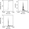 |
Fig. 1 Evolution of Neptune’s semimajor axis, eccentricity, and inclination from the original integration during 100 My around the instability phase. The evolution after 0.7 Gy is similar to that in Fig. 3. |
The planetary semimajor axes at the beginning and end of the integration are shown in Table 2. Although the planets stop at different positions from their current ones, this kind of integration has the advantage of showing a planetary migration induced by the perturbation of the particles and not by a synthetically applied force. A planetesimal in our simulation has a mass roughly three times smaller than Pluto’s. If we consider a cumulative size distribution for the planetesimals as d-4, where d is the planetesimal’s radius, and that there were 1000 Plutos in the original disk, this disk would have ~5000 objects with mass equal to or larger than the planetesimal mass in the simulation. This corresponds to ~2700 times Pluto’s mass, which corresponds to 5.4ME or 13.5% of the disk’s mass. Considering that this mass is composed of objects whose size is equal to and larger than those considered in the simulations, we conclude that a fraction larger than 13.5% of the disk’s mass will be composed of objects that will cause a similar stochasticity to the simulated disk. So although our assumed disk is not totally realistic, it likely mimics the migration of the planets more accurately than through a synthetically imposed force. Thus, some processes like the trapping of particles into mean motion resonances with the planets is likely simulated more realistically than in a model where the planets migrate through an artificially constructed force. In fact, several captures of planetesimals like Neptune trojans are noticed during the evolutions of planets and particles. Figure 2 shows an example of a planetesimal that was temporarily trapped during Neptune’s migration and kept trapped during ~100 My. There was a total of 45 planetesimals that were NTs continuously for more than 5 My after the planetary instability phase based on the libration of the 1:1 resonant angle. The longest time an object spent as a Neptune trojan was 312 My, but there were no trojans left at the end of the integration after t = 1.5 Gy. In fact, this would be expected as the total mass of Neptune trojans is estimated at 1.2 × 10⁻⁵ME. Since this is less than 1 / 60 000 of the disk mass, it is not expected that in the end we would have a surviving Neptune trojan from a disk with 60 000 particles. We could possibly have one Neptune trojan at the end of such a simulation if we included 20 times more particles in the integration, which is prohibitive with the current computation capabilities.
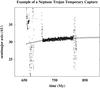 |
Fig. 2 Semimajor axis evolution of Neptune and a planetesimal that was temporarily trapped in coorbital resonance with Neptune. |
Thus, we developed a method for increasing the number of trojans in a simulation. First, we considered the original integration as the basis for new synthetic numerical integrations. We computed the migration rate of all four planets from the original integration, after 670 My, when the planets were already free from close encounters. This was done by computing an average semimajor axis for every interval of 106 yrs and then computing the variation in this mean semimajor axis between each interval. Once these migration rates were obtained, we reversed the sense of migration and performed a backward numerical integration2 of the four giant planets with initial conditions like those of their current orbits (Julian date 2 454 200.5). The integration was carried on for the whole time that the migration rates were computed. The orbital elements of the planets at the end of this backward integration were the new initial conditions for new forward numerical integrations where we applied the original migration rates mentioned above to mimic the original integration, but with planets ending at their current positions. Figure 3 shows the evolution of the semimajor axis and eccentricity of Neptune and Uranus for a typical forward run, which mimics the original run, but the planets are parked at their approximate current orbits. Table 3 shows the semimajor axis, eccentricity, and inclination of the planets for the synthetic runs. The differences between each of the forward runs are just the clones of the trojans introduced into each of the integrations.
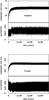 |
Fig. 3 Evolution of the semimajor axis and eccentricity of Neptune and Uranus for a typical synthetic run. |
Two hundred clones were created for each of the 45 NTs coming from the original integration. This was implemented by adding a random angle in degrees between −0.05 and 0.05 to the mean longitude of the original trojan. The 45 original trojan orbital elements are those from the original integration taken at the average time of their evolution as NT. When we thus choose the NTs to be cloned, we are supposing that the very trapping process is mostly dependent on the mutual positions of Neptune and the trapped particle and minimally dependent on the influence of the other planets. After choosing the 45 original trojans, we shifted their semimajor axes to make it a trojan for the normalized Neptune in the synthetic integrations. We also referred the longitudes to the new Neptune longitudes. Eccentricities and inclinations were the same as those in the original integration. These procedures may not be accurate enough to ensure the right libration amplitude for the cloned NTs. Although the initial resonant angle is chosen to be the same for the original particle and for its clones, the problem is that their evolutions can be fairly different implying different libration amplitudes. This occurs because the evolution has an important dependence on the positions of the other planets and there is no way to mimic the same planetary configuration both for the original integration and the synthetic ones. To cope with this, we introduced the cloned particles as close to Neptune as the closest distance of the original particle with Neptune. At this point most of the perturbation comes from this planet and the differences in libration amplitudes between the original particle and the cloned ones were shown to stay within acceptable limits.
Figure 4 shows a typical evolution of the libration angle for the original particle and the cloned ones. As long as the creation of the clones presupposes the use of random numbers, this differentiates the runs at first with respect to the particles. But since a close encounter of a particle with a planet makes the hybrid version of the MERCURY integrator enter into a classical variable step length integration, this is sufficient to produce different orbital elements for the planets at the end of each of the synthetic integrations.
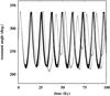 |
Fig. 4 Evolution of the libration angle for one of the NTs in the original integration (line) and their cloned counterparts in the synthetic integrations (dots). |
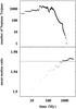 |
Fig. 5 Variation in the number of NTs and the mean motion ratio between the ice planets, for a simulation where the mean motion ratio superseded the real ratio, represented by the horizontal line. |
Before we present the results of these runs, we must point out that the forward numerical integrations always exhibited a larger absolute value of the variation in semimajor axes than the backward integration. The reason for this must lie in the fact that forward integrations are associated with divergent orbits and the crossing of mean motion resonances in divergent orbits implies jumps in the semimajor axes of pairs of planets at crossing resonances. For convergent orbits (backward integration) the mean motion resonance crossing is usually associated with a break in the migration of the pair of planets that crossed the resonance. Although during the tail of the migration as is considered here there is no low order mean motion resonance crossing, there are always high order mean motion resonance crossings and they must be responsible for the wider range of values of the semimajor axes of the forward migrations. The mean motion ratio for the current orbits of Neptune and Uranus3 is 1.961, computed from a numerical integration of the giant planets starting from the same orbital elements as those used above to start the backward integration. After the backward integration and several forward integrations, these mean motion ratios at the end of those forward integrations were in the range 1.963−1.968. Although not a very large difference from the actual ratio, if we take into account that the pair of ice giants are close to their 1:2 MMR, the stability of the trojans may be (and indeed is) sensible to these small variations in the mean motion ratio.
Initial semimajor axis, eccentricity and inclination for the planets in the synthetical runs.
So our first example is a run where Uranus and Neptune stopped at a period ratio of 1.966. This integration, like all the other synthetic ones, is performed for ~3.83 Gy, which yields about 4.5 Gy after summing up with the initial phase of the original run up to the point where planetary instabilities have calmed down at 0.67 Gy. Figure 5 shows the variation in this ratio during the migration and the evolution of the number of trojans. The spikes are related to the times where the trojan clones are introduced. We can see that after about 1.5 Gy there were no trojans left. This means that the mass of the Neptune trojans would be smaller than 3.5 × 10⁻⁶ME, which is the mass represented by each particle and is possibly too small compared to the estimated mass for the NTs. Thus, we see that not going past the current mean motion ratio between the ice giants may be important. We tried several forward numerical integrations with the above-mentioned migration rates and tentatively found that using a reducing factor of 0.97 in Neptune’s migration rate would make the Uranus-to-Neptune mean motion ratio stop near their present ratio. That is how the synthetic numerical integrations are undertaken as described in the next section.
3. Results
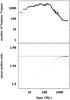 |
Fig. 6 Variation in the number of NTs and the mean motion ratio between the ice planets, for integration #1 in Table 4. |
Neptune trojan data for the end of the synthetic runs at 3.8 Gy.
We undertake five different numerical integrations like the synthetic one described at the end of the previous section. Although we use the same migration rates for all five integrations, each integration has a different set of planetary evolutions, as explained in the previous section. In addition to considering the reducing factor for Neptune’s migration as mentioned above, we also stopped the migration whenever the Neptune-to-Uranus period ratio reached the current one at 1.961. Table 4 gives a summary of the results at the end of the five integrations. Figure 6 shows the evolution of the number of NTs and the Neptune-to-Uranus mean motion ratio for one of the runs (#1 in Table 4.)
Since each particle in the original integration carried 7 × 10⁻⁴ME and it was cloned 200 times, it is easy to compute the total mass of Neptune trojans from their total final number in each of the five integrations. The obtained mass in Table 4 is around five times larger than the estimated mass for the NTs.
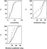 |
Fig. 7 Cumulative distribution of the eccentricities, inclinations, and libration amplitudes of the NTs obtained in the simulations compared with the real distributions (dots). |
Figure 7 shows the cumulative distribution of eccentricities, inclinations, and libration amplitudes for all five integrations compared to the distribution for real NTs. The libration amplitudes are taken from Parker (2015). The fraction of Neptune trojans obtained by the simulations with inclinations between 0° and 10°, 10° and 20°, and above 20° are respectively 0.05, 0.30, and 0.65. On the other hand, for the real NTs these fractions are 0.36, 0.18, and 0.45. The skewness toward larger inclination noticed for the simulation distribution can be explained: most surveys are undertaken near the ecliptic, which favors the discovery of less inclined objects. In fact, these results show that Neptune trojans with highly inclined orbits are a natural outcome in a model where the planetesimals are dynamically excited. This result differs considerably from those of Parker (2015), where NTs that are inclined enough are not obtained unless a pre-heated disk is assumed. The reason for this may be that our original integration has a migration timescale of ~150 My, whereas Parker (2015) just considers migration timescales in the range 1−10 My. A slower migration of Neptune is important in order to make it encounter a much more excited disk with larger planetesimal inclinations. As for the libration mode, of a total of 233 trojans in all five integrations, 82 were trailing and 151 were leading. This yields a ratio L4/L5 of 1.7, not too distant from the real ratio of 4 considering that trailing NTs are harder to observe since they are outshined by the Milky Way. The distribution of libration amplitudes of the real NTs shows a clustering around 20°, which is not noticed in our simulation distribution, although the range of values in both cases are similar (Parker 2015). The eccentricities are agree closely with the distributions from the real NTs.
4. Has Neptune ever been more distant than it is today?
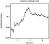 |
Fig. 8 Neptune’s averaged semimajor axis evolution from the original integration, normalized so as to make Neptune park at its current semimajor axis. |
In numerical simulations of the evolution of the orbits of the giant planets and planetesimals in a planetary instability model, the planets always show a secular trend by which the Saturn, Uranus, and Neptune migrate outward and Jupiter migrates inward, as in our original integration. Added to the secular variation, there is a random variation in the semimajor axes of the planets both outward and inward. A possible consequence is that at some time in the past Neptune may have been more distant than it presently is. Figure 8 shows the normalized evolution of Neptune’s semimajor axis from the original integration. This figure suggests that about ~1.6 Gy ago Neptune could have been ~0.02 au farther from the Sun than today4. This corresponds to a mean motion ratio with Uranus at 1.963 instead of the present ratio at 1.961 (neglecting Uranus’ much smaller migration). Although a small difference, this possible past mean motion ratio places Neptune and Uranus closer to their 1:2 mean motion resonance. As commented in the introduction, this could have had an important effect on the stability of Neptune’s trojans. We undertook a few experiments to check the above hypothesis. First we present the result of a numerical integration similar to the five presented above with the same migration parameters as those, but with the exception that we did not turn off the migration when Neptune and Uranus reached their current mean motion ratio. Figure 9 shows both the evolution of the ice planets’ mean motion ratio and the number of trojans alive in the integration. At the end, there were 14 trojans left in the integration corresponding to ~5 × 10⁻⁵ME, which is closer to the real estimated mass for the NTs than the mass obtained for simulations in which Neptune does not migrate farther than its present distance from the Sun.
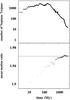 |
Fig. 9 Variation in the number of NTs and the mean motion ratio between the ice planets for a simulation where the mean motion ratio ended very close to the real ratio, after being above it in the past. |
 |
Fig. 10 Variation in the number of NTs for a continuation of integration #4 for a mean motion ratio of 0.002 (upper panel) or 0.004 (lower panel) above (forward) and below (backward) the real ratio. |
In the second experiment we considered the final result of integration #4 (see Table 4) and continued the integration for an additional ~700 My in four other integrations, yielding a total of 4.5 Gy from the beginning of the synthetic runs or 5.2 Gy from the beginning of the original run, even though absolute time is not important here. In two of them we considered an outward migration of Neptune with a migration rate of ~0.22 au/Gy and in the other two we considered the same absolute value of the migration rate in an inward migration. For one pair of integrations, Neptune migrates until the ice giants mean motion ratio reaches 0.002 above/below its current value. For the other pair, Neptune migrates until the mean motion ratio reaches 0.004 above/below its current value. After reaching these mean motion ratios (1.957, 1.959, 1.963, 1.965), Neptune evolves without migration. Figure 10 shows that the loss of Neptune trojans when the ice planets approach their 1:2 mean motion resonance is much greater than when there is a departure from the mean motion resonance by an equal amount. The vertical lines define the time when the migration ceased.
To complement the results discussed in the previous text, we tested the stability of NTs for different period ratios of Uranus and Neptune (for an analysis of the stability of NTs for the present orbits of Uranus and Neptune, see Zhou et al. 2009, 2011). In these tests with no planetary migration, all four giant planets were included. We first used their current orbital configuration and distributed a large number of test particles near the leading Lagrangian point. The initial orbits of the test particles are discussed below. The results of the simulation with current orbits of planets represent a reference case that shows the stability of trojan orbits in the present solar system. We then performed several additional simulations where the semimajor axis of Neptune was shifted outward from its current value (mean a = 30.11 au) by Δa.
The test particle orbits were randomly distributed with 29.6 <a< 30.6 au and e< 0.25. We used different orbital sets with 5000 test orbits in each set having the same initial inclination (i = 0, 10°, 20°, or 30°). The other orbital elements were set such that λ−λN = 60°, ϖ = 0, and Ω = 0, where λ and λN are the mean longitudes of a test particle and Neptune, and ϖ and Ω are the perihelion and nodal longitude of a test particle. This choice assures that each set of orbits intersects the leading Lagrangian point in a well-defined manner. Also, initial a−aN is a good proxy for the amplitude of the semimajor axis oscillations.
The orbits of four outer planets and test particles were numerically integrated by the standard Swift integrator (Levison & Duncan 1994). We used a 0.5 yr timestep which gives roughly 22 steps in one orbital period of Jupiter. This resolution is high enough to have reliable results. The integrations were stopped at time t = 100 Myr. At this point, we selected all test particles that remained on stable orbits near the leading Lagrangian point. The initial orbits of these stable particles are plotted in Figs. 11 and 12. These figures show that in the current solar system, Neptune trojans with i = 10° are stable up to e ≃ 0.1 (Fig. 11) and those with i = 20° are stable up to e ≃ 0.2 (Fig. 12).
When Neptune’s orbit is altered by Δa ≃ 0.02−0.03 au, the eccentricity spread of stable orbits decreases considerably (Figures 11 and 12). In both cases, the orbits with eccentricities e ≥ 0.05 become unstable. We did not investigate the cause of the instability in detail, but we suspect that it may have something to do with the resonance between the σUN = 2λN−λU (small inequality, λU is the mean longitude of Uranus), and the libration of σ = λ−λN. The libration period of σ is typically slightly shorter than 10 000 yr, and the exact value depends on the libration amplitude, e and i of the test particle. The current circulation period of σUN is roughly 4200 yr, but this period is very sensitive to Δa, and it may easily be increased.
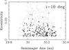 |
Fig. 11 Results of a stability survey near the leading Lagrangian point of Neptune. The small dots show the initial orbits of particles with i = 10° that remained stable for 100 Myr. The bold dots show the stable orbits for a shifted semimajor axis of Neptune (Δa = 0.02 au). |
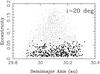 |
Fig. 12 Results of a stability survey near the leading Lagrangian point of Neptune. The small dots show the initial orbits of particles with i = 20° that remained stable for 100 Myr. The bold dots show the stable orbits for a shifted semimajor axis of Neptune (Δa = 0.03 au). |
It is noted in Figs. 11 and 12 that the eccentricities that remain are smaller than those obtained in the above synthetic simulations with migration. We understand that the reality is slightly more complex than the simple tests we have done with no migration. For example, it is possible to imagine that the population is initially cut at e< 0.05, but then, during the subsequent evolution, eccentricities become somewhat mixed up such that particles evolve from e< 0.05 to e> 0.05.
We thus suggest that the 2:1 resonance between σ and σUN may be limiting the stability to e<ecrit, where the critical eccentricity ecrit is a function of i and Δa. This has an exact analog in the Jupiter-Saturn system where Saturn’s trojans with small libration amplitude and eccentricity above a critical value are unstable owing to a resonance between the libration angle and the great inequality (2λJ−5λS, where λJ and λS are Jupiter’s and Saturn’s mean longitude (Nesvorný & Dones 2002).
A detailed study of the instability cause is left for future work. Here we just point out that a shift of Δ = 0.02−0.03 au corresponds to a change in the Uranus-Neptune period ratio of 0.002−0.003, which is exactly the sort of period shift discussed in the migration simulations in the previous section. Finally, we find that the Δa> 0.02−0.03 au is needed to destabilize orbits with i = 30°. If the shift is too large, however, orbits become more stable and the stability island regains its original size as in the present solar system. This result highlights the sensitivity of NT stability to the exact period ratio of Uranus and Neptune.
5. Conclusions
We performed a numerical simulation of the migration of the giant planets in a planetesimal disk. We found that several planetesimals were trapped in coorbital resonance with Neptune, but at the end of the integration at 4.5 Gy, no NT was left. To manage this, we cloned each temporary original TN 200 times and ran synthetic integrations keeping the same migration rates of the planets as in the original one. In these new integrations, several planetesimals remained in coorbital resonance with Neptune until 4.5 Gy. The total mass that corresponds to these surviving trojans is about 1.6 × 10⁻⁴ME and the distribution of eccentricities, inclinations, and libration amplitudes are respectively 0.007 to 0.173, 4.9° to 32.9°, and 6.9° to 64.3°, which matches quite well the orbital distribution of real Neptune trojans. The mass left at the end of the integrations is about five times larger than the NTs estimated mass.
In some integrations where Neptune migrated a little farther than its present position and then migrated back to its current position, it was found that as the Neptune-to-Uranus mean motion ratio approached 2 many more trojans became unstable during the integration. In a specific run where the Neptune-to-Uranus mean motion ratio reached 1.963 and decreased to the present value (1.961), many more trojans escaped the coorbital resonance with Neptune and in the end there were NTs equivalent to a mass of 5 × 10⁻⁵ME, closer to the real estimated mass (3 × 10⁻⁵ME). Since planetary migration in an instability model shows the possibility that in the past Neptune was a little farther from the Sun than it is today, we should consider this possibility to explain the apparent dearth of NTs as compared to those produced by a planetary instability migration model where Neptune never goes beyond its current position. On the other hand, it is possible that the method employed in this paper may favor a greater stability of the NTs as we are replacing a migration induced by planetesimal encounters with a synthetically smoother migration, even though it resembles the original one. It is also possible that a migration produced by a cold disk might induce a smaller amount of NTs trappings, which would indicate a possible signature of this latter migration model. On the other hand, this model would also have to be tested against the orbits of the NTs, in particular with respect to their inclinations.
This and other numerical integrations described in this paper were done with a modified version of the MERCURY hybrid integrator to allow secular migration of the planets.
Mean motion ratios are always computed with averaged semimajor axes.
The first author performed a similar integration with the difference that he included a planetary mass solar companion. In this case Neptune was 0.003 au farther than its final position. He did another integration starting with 1000 planetesimals and whenever the number of planetesimals reached 500, he cloned each one so that he always had between 500 and 1000 particles in the integration. In this case Neptune was 0.09 au farther away from its final position. These examples provide extra evidence that Neptune’s migration beyond its current position is a relevant possibility.
References
- Alexandersen, M., Gladman, B., Kavelaars, J. J., et al. 2014, ArXiv e-prints [arXiv:1411.7953] [Google Scholar]
- Brasser, R., Morbidelli, A., Gomes, R., Tsiganis, K., & Levison, H. F. 2009, A&A, 507, 1053 [NASA ADS] [CrossRef] [EDP Sciences] [Google Scholar]
- Chambers, J. E. 1999, MNRAS, 304, 793 [NASA ADS] [CrossRef] [MathSciNet] [Google Scholar]
- Fraser, W. C., Brown, M. E., Morbidelli, A., Parker, A., & Batygin, K. 2014, ApJ, 782, 100 [NASA ADS] [CrossRef] [Google Scholar]
- Gomes, R., Levison, H. F., Tsiganis, K., & Morbidelli, A. 2005, Nature, 435, 466 [NASA ADS] [CrossRef] [PubMed] [Google Scholar]
- Horner, J., & Lykawka, P. S. 2012, MNRAS, 426, 159 [NASA ADS] [CrossRef] [Google Scholar]
- Kavelaars, J. J., Jones, R. L., Gladman, B. J., et al. 2009, AJ, 137, 4917 [NASA ADS] [CrossRef] [Google Scholar]
- Levison, H. F., & Duncan, M. J. 1994, Icarus, 108, 18 [NASA ADS] [CrossRef] [Google Scholar]
- Lykawka, P. S., & Horner, J. 2010, MNRAS, 405, 1375 [NASA ADS] [Google Scholar]
- Lykawka, P. S., Horner, J., Jones, B. W., & Mukai, T. 2009, MNRAS, 398, 1715 [NASA ADS] [CrossRef] [Google Scholar]
- Morbidelli, A., Levison, H. F., Tsiganis, K., & Gomes, R. 2005, Nature, 435, 462 [NASA ADS] [CrossRef] [PubMed] [Google Scholar]
- Morbidelli, A., Brasser, R., Tsiganis, K., Gomes, R., & Levison, H. F. 2009, A&A, 507, 1041 [NASA ADS] [CrossRef] [EDP Sciences] [Google Scholar]
- Nesvorný, D. 2011, ApJ, 742, L22 [NASA ADS] [CrossRef] [Google Scholar]
- Nesvorný, D., & Dones, L. 2002, Icarus, 160, 271 [NASA ADS] [CrossRef] [Google Scholar]
- Nesvorný, D., & Morbidelli, A. 2012, AJ, 144, 117 [NASA ADS] [CrossRef] [Google Scholar]
- Nesvorný, D., & Vokrouhlický, D. 2009, AJ, 137, 5003 [NASA ADS] [CrossRef] [Google Scholar]
- Parker, A. H. 2015, Icarus, 247, 112 [NASA ADS] [CrossRef] [Google Scholar]
- Tsiganis, K., Gomes, R., Morbidelli, A., & Levison, H. F. 2005, Nature, 435, 459 [NASA ADS] [CrossRef] [PubMed] [Google Scholar]
- Zhou, L.-Y., Dvorak, R., & Sun, Y.-S. 2009, MNRAS, 398, 1217 [NASA ADS] [CrossRef] [Google Scholar]
- Zhou, L.-Y., Dvorak, R., & Sun, Y.-S. 2011, MNRAS, 410, 1849 [NASA ADS] [Google Scholar]
All Tables
Initial semimajor axis, eccentricity and inclination for the planets in the synthetical runs.
All Figures
|
Fig. 1 Evolution of Neptune’s semimajor axis, eccentricity, and inclination from the original integration during 100 My around the instability phase. The evolution after 0.7 Gy is similar to that in Fig. 3. |
| In the text | |
|
Fig. 2 Semimajor axis evolution of Neptune and a planetesimal that was temporarily trapped in coorbital resonance with Neptune. |
| In the text | |
|
Fig. 3 Evolution of the semimajor axis and eccentricity of Neptune and Uranus for a typical synthetic run. |
| In the text | |
|
Fig. 4 Evolution of the libration angle for one of the NTs in the original integration (line) and their cloned counterparts in the synthetic integrations (dots). |
| In the text | |
|
Fig. 5 Variation in the number of NTs and the mean motion ratio between the ice planets, for a simulation where the mean motion ratio superseded the real ratio, represented by the horizontal line. |
| In the text | |
|
Fig. 6 Variation in the number of NTs and the mean motion ratio between the ice planets, for integration #1 in Table 4. |
| In the text | |
|
Fig. 7 Cumulative distribution of the eccentricities, inclinations, and libration amplitudes of the NTs obtained in the simulations compared with the real distributions (dots). |
| In the text | |
|
Fig. 8 Neptune’s averaged semimajor axis evolution from the original integration, normalized so as to make Neptune park at its current semimajor axis. |
| In the text | |
|
Fig. 9 Variation in the number of NTs and the mean motion ratio between the ice planets for a simulation where the mean motion ratio ended very close to the real ratio, after being above it in the past. |
| In the text | |
|
Fig. 10 Variation in the number of NTs for a continuation of integration #4 for a mean motion ratio of 0.002 (upper panel) or 0.004 (lower panel) above (forward) and below (backward) the real ratio. |
| In the text | |
|
Fig. 11 Results of a stability survey near the leading Lagrangian point of Neptune. The small dots show the initial orbits of particles with i = 10° that remained stable for 100 Myr. The bold dots show the stable orbits for a shifted semimajor axis of Neptune (Δa = 0.02 au). |
| In the text | |
|
Fig. 12 Results of a stability survey near the leading Lagrangian point of Neptune. The small dots show the initial orbits of particles with i = 20° that remained stable for 100 Myr. The bold dots show the stable orbits for a shifted semimajor axis of Neptune (Δa = 0.03 au). |
| In the text | |
Current usage metrics show cumulative count of Article Views (full-text article views including HTML views, PDF and ePub downloads, according to the available data) and Abstracts Views on Vision4Press platform.
Data correspond to usage on the plateform after 2015. The current usage metrics is available 48-96 hours after online publication and is updated daily on week days.
Initial download of the metrics may take a while.