| Issue |
A&A
Volume 592, August 2016
|
|
|---|---|---|
| Article Number | A73 | |
| Number of page(s) | 6 | |
| Section | The Sun | |
| DOI | https://doi.org/10.1051/0004-6361/201527145 | |
| Published online | 28 July 2016 | |
The influence of helical background fields on current helicity and electromotive force of magnetoconvection
Leibniz-Institut für Astrophysik Potsdam, An der Sternwarte 16, 14482 Potsdam, Germany
e-mail: This email address is being protected from spambots. You need JavaScript enabled to view it.
; This email address is being protected from spambots. You need JavaScript enabled to view it.
Received: 8 August 2015
Accepted: 29 April 2016
Abstract
Motivated by the empirical finding that the known hemispheric rules for the current helicity at the solar surface are not strict, we demonstrate the excitation of small-scale current helicity by the influence of large-scale helical magnetic background fields on nonrotating magnetoconvection. This is shown within a quasilinear analytic theory of driven turbulence and by nonlinear simulations of magnetoconvection that the resulting small-scale current helicity has the same sign as the large-scale current helicity, while the ratio of both pseudoscalars is of the order of the magnetic Reynolds number of the convection. The same models do not provide finite values of the small-scale kinetic helicity. On the other hand, a turbulence-induced electromotive force is produced including the diamagnetic pumping term, as well as the eddy diffusivity but, however, no α effect. It has thus been argued that the relations for the simultaneous existence of small-scale current helicity and α effect do not hold for the model of nonrotating magnetoconvection under consideration. Calculations for various values of the magnetic Prandtl number demonstrate that, for the considered diffusivities, the current helicity increases for growing magnetic Reynolds number, which is not true for the velocity of the diamagnetic pumping, which is in agreement with the results of the quasilinear analytical approximation.
Key words: magnetohydrodynamics (MHD) / magnetic fields / convection / Sun: activity
© ESO, 2016
1. Introduction
An increasing number of observations concerns the small-scale current helicity:  (1)at the solar surface, all showing that it is negative (positive) in the northern (southern) hemisphere (Hale 1927; Seehafer 1990; Rust & Kumar 1994; Abramenko et al. 1996: Bao & Zhang 1998; Pevtsov 2001; Kleeorin et al. 2003; Zhang et al. 2010, 2012). Here the notation b denotes the fluctuating parts of the total magnetic field in the form
  . It became clear that the scalar quantity (1) shows a strict equatorial antisymmetry with signs which do not change from cycle to cycle. We note that for the linear α2 dynamo, as well as the simple αΩ dynamos, the large-scale helicity,
  similar to (1), also shows equatorial antisymmetry in accordance with
  (Steenbeck & Krause 1969). The fact that for flux transport αΩ dynamos the relation is much more complicated (positive correlation only during the cycle minima) indicates that a direct relation
  does not necessarily exist. It is nevertheless important that all the mentioned scalars, such as helicities and α effect are pseudoscalars, which may be related to each other.
There are many theoretical studies where both the current helicity and the α effect are derived as consequences of the existence of the pseudoscalar g·Ω in rotating convection zones with g as the (radial) direction of stratification. Yet it is shown in this paper that the current helicity can also be produced, even without rotation, if the convection is influenced by a magnetic background field that is helical. Then the question is whether the same constellation would also lead to a turbulence-induced electromotive force via an α effect as suggested by the relation  (2)of Keinigs (1983). This is based on the existence of homogeneous and stationary turbulence with finite kinetic helicity (Seehafer 1996), where these conditions are obviously not fulfilled if one of the magnetic field components is inhomogeneous. Pouquet & Patterson (1978) presented the relation
  (3)which also means that even turbulent fluids with vanishing kinetic helicity, but finite small-scale current helicity, should possess an α effect but with an opposite sign as in Eq. (2).
Studies by Yousef et al. (2003), Blackman & Subramanian (2013) and Bhat et al. (2014) are concerned with the dissipation of helical and nonhelical large-scale background fields under the influence of a nonhelical turbulent forcing. In these papers, it is shown that the kinetic helicity is dominated by the current helicity, which is confirmed by our quasilinear calculations for forced turbulence and the nonlinear simulations of magnetoconvection under the influence of a large-scale helical field. In contradiction to the relation (3), both the quasilinear approximation and nonlinear simulations provide reasonable values for the current helicity, but they do not lead to a finite α effect.
2. The current helicity
To find the current helicity that is due to the interaction of a prescribed stochastic velocity u(x,t) and a large scale magnetic field  it is sufficient to solve the induction equation
  (4)where the fluctuating magnetic field may be written as
  . The influence of field gradients on the mean current helicity (1) at linear order is governed by
  (5)where the prescribed inhomogeneous mean magnetic field
  has been introduced in the form
  with the notation
  and with Bjj = 0. It follows
  , which here may form the only pseudo-scalar in the system.
To solve Eq. (5), we use the inhomogeneous Fourier modes  (6)This is a standard procedure that yields
  (7)(Rüdiger 1975) from which the small-scale current helicity
 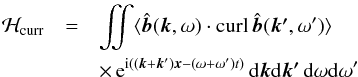 (8)can easily be formed. A homogeneous and isotropic turbulence field with the spectral tensor
 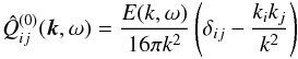 (9)may be postulated where the positive spectrum E gives the intensity of the fluctuations. After several manipulations, the final expression can be derived from (8) and (9)
 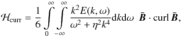 (10)which describes the induction by turbulence in a background field with helical geometry. As is necessary, the effect vanishes in the vacuum (η → ∞). In the high-conductivity limit (η ≪ urmsℓcorr), the integral in (10) only exists after multiplication with η so that
 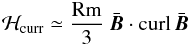 (11)linearly scales with the magnetic Reynolds number Rm = urmsℓcorr/η. Within the low-conductivity limit, as the opposite approximation, the small-scale current helicity scales with Rm2, as does the normalized magnetic energy
  in the theory of Bräuer & Krause (1974).
With (11) the relation (3) would lead to 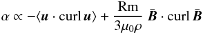 (12)for the α effect in the high-conductivity limit and for weak magnetic fields (Blackman & Brandenburg 2002; Brandenburg & Subramanian 2005).
With our approximations (quasilinear equations, forced turbulence, no rotation) the ratio of the two helicities corresponds to the ratio of both the magnetic energies. Equation (11) requires the same sign for the small-scale and the large-scale current helicities. With (2), one finds  which contradicts the above mentioned observations, which in the simple α2 dynamos
  . The only solution to this dilemma is that nonrotating convection under the influence of helical large-scale fields may produce small-scale current helicity but it does not generate an α effect.
If calculated under the same analytical assumptions as the current helicity (1), the kinetic helicity ⟨ u·curl u ⟩ provides zero. Blackman & Subramanian (2013) find that during the turbulence-induced decay of helical large-scale fields the kinetic helicity remains unchanged. In the quasilinear approximation, the helicity expression, which is due to the background fields, also vanishes. magnetohydrodynamic (MHD) turbulence under the influence of a helical large-scale field is thus suspected of generating finite values of current helicity but no kinetic helicity. The question is whether on this basis, and after the relations (2) and/or (3), nonlinear simulations of convection in a stratified plasma also generate current helicity but both the kinetic helicity and the α effect disappear.
In a previous paper we simulated magnetoconvection under the influence of a uniform vertical magnetic field to produce finite values of cross helicity (Rüdiger et al. 2012, Paper I hereafter). In this paper the helical magnetic background field 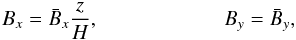 (13)with uniform values of
  and
and  has been applied as an initial field to probe the possible production of both small-scale kinetic and current helicity. In the computational layer, the vertical coordinate z runs from 0 to 2H, while the convection zone is located in [H,2H]. The value of the initial electric current is
  , hence the initial value of the large-scale current helicity is
  .
.
The numerical value of  developes during the simulation as the code also implicitly solves the mean-field equations (including the advection term discussed below). Also under the influence of the boundary conditions for the magnetic field, the helicity becomes depth-dependent but its (positive) sign is always preserved. Averaged over the horizontal plane, the linear dependence of
  on the product
  is also numerically reproduced for the evolved large-scale current helicity. In the bulk of the convection box the numerical values of the maxima of the latter are 70 for
  and 150 for
  .
.
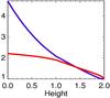 |
Fig. 1 Snapshots of temperature (red lines) and density (blue lines) during the run for |


The compressible MHD equations have been solved with the nirvana code (Ziegler 2004) in a Cartesian box with gravitation along the negative z-axis. The box is periodic in the horizontal directions and all mean-field quantities are averaged over the horizontal plane. For the Prandtl number and the magnetic Prandtl number, a common value is fixed at 0.1. As in Paper I, the velocities are used in units of cac/ 100 where cac is the speed of sound at the top of the convection box (see Fig. 1). Correspondingly, the magnetic fields are given in units of  with μ0 = 4π. We again assume an ideal, fully ionized gas heated from below and kept at a fixed temperature at the top of the simulation box. As in Paper I, the dimensionless Rayleigh number is fixed at 107. Periodic boundary conditions apply at the horizontal boundaries. The upper and lower boundary are perfect conductors so that for the total magnetic fields
  (14)which is similar to the stress-free conditions of the velocity, dux/ dz = duy/ dz = uz = 0. At the inner boundary the heat-flux is fixed. In Paper I, we find that for very weak magnetic fields the rms-value of the convection velocity in the used units is about 8 (see also the left panel of Fig. 2 below). This means that with the dimensionless η = 0.06 the global magnetic Reynolds number slightly exceeds 100, which is larger by definition than the local magnetic Reynolds number Rm = urmsℓcorr/η introduced above.
We start to compute the intensities of the magnetoconvection  and
and  (Fig. 2). The velocity at the top of the convective box results in ≲10% of the surface value of the sound speed, which for the Sun is about 10 km s-1. The given time averages and vertical averages in z = [ 1,2 ] of all snapshots are taken as the characteristic values of the quantities. The differences of the velocity dispersion to those given in Paper I, where much weaker vertical fields have been applied, are very small. The magnetic quenching of the velocity fields does exist, but it is weak. However, the ratio
  is strongly affected by the mean magnetic field. While its value is about 30 for the vertical field
  , in Paper I the helical field
  only allows q values of order unity. We note also that
  , so that, with density values taken from Fig. 1, the convection is not magnetic-dominated. Contrary to that, we demonstrate that, nevertheless, the current helicity strongly dominates the kinetic helicity.
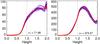 |
Fig. 2 Turbulence-intensities |


For the same model, the correlation coefficients,  (15)for the kinetic helicity and the current helicity, have been computed (Fig. 3). The numerical values differ greatly. While the fluctuations of b and curl b are well correlated, this is not the case for the flow field.
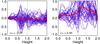 |
Fig. 3 As in Fig. 2, but for the correlation coefficients ckin (left) and ccurr (right). The numbers below the graphs are the volume averages of the coefficients over the whole convective domain. The average of all snapshots in both cases is below unity. |
A systematic behavior of the z-profile also does not exist. In accordance with the analytic quasilinear calculations, magnetoconvection that is subject to helical background fields does not generate small-scale kinetic helicity, but it generates small-scale current helicity.
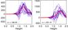 |
Fig. 4 Small-scale current helicity ⟨ b·curl b ⟩ the result of the large-scale current helicity |


The behavior of the magnetoconvection complies with the above analytical result of the incapability of large-scale helical fields to produce small-scale kinetic helicity from nonhelical turbulence, and this corresponds with the results of Blackman & Subramanian (2013) and Bhat et al. (2014), who find the helicities as magnetic-dominated in their simulations of decaying helical background fields under the influence of nonhelically driven turbulence.
After (11), we expect the current helicity numerical values to exceed  , which is indeed confirmed by the simulations (Fig. 4). The average number in the right plot is just twice the number in the left plot, demonstrating the linear run of the correlation with the large-scale helicity. The relation (11), which linearly connects the small-scale current helicity with the large-scale current helicity, can thus be considered as being fulfilled by the numerical simulations. The numerical value between the two helicities and its relation to the magnetic Reynolds number is discussed below in Sect. 3.2.
3. The electromotive force
The same magnetoconvection model is used to calculate the turbulence-induced electromotive force. As electric currents exist in the convection zone, this will certainly contain tensorial components of magnetic diffusion. The question is whether an electromotive force along the magnetic field also occurs, which must be interpreted as an α effect. Surprisingly, the answer is that no α effect is generated by the convection that is influenced by the helical magnetic background field (13). Since simultaneously current helicity without kinetic helicity exists, Eq. (3) cannot be correct for all possible turbulence fields.
The electromotive force ℰ = ⟨ u × b ⟩ in a turbulent plasma is a polar vector. To express linearly by the axial mean magnetic field vector  , then only the formulation
 (16)is possible if pseudoscalars, such as g·Ω or
  , are not available. Without global rotation, an α effect in the formulation
  does not occur in the linear relation (16). The parameter ηT describes the turbulence-induced eddy diffusivity in the fluid, while the vector γ gives a velocity which transports (“pumps”) the large-scale magnetic field downward for positive γz. If, however, terms that are nonlinear in are included in the heuristic expression (16), then the extra terms
![Mathematical equation: \begin{equation} \vec{\cal E}\!=....+{\hat\eta}\ \ \bigg(\!\bar{\vec{B}}^2 \, {\rm curl}\, \bar{\vec{B}} + \frac{1}{3} \bigg[\nabla \bar{\vec{B}}^2 + (\bar{\vec{B}}\cdot\nabla) \bar{\vec{B}}\bigg]\times \bar{\vec{B}}\!\bigg) \label{E3} \end{equation}](/articles/aa/full_html/2016/08/aa27145-15/aa27145-15-eq96.png) (17)occur within the second-order-correlation approximation (Kitchatinov et al. 1994). The first term of the right hand side represents the known magnetic influence on the eddy diffusivity, while the second one forms a magnetic-induced pumping effect. There is no term
(17)occur within the second-order-correlation approximation (Kitchatinov et al. 1994). The first term of the right hand side represents the known magnetic influence on the eddy diffusivity, while the second one forms a magnetic-induced pumping effect. There is no term  representing an α effect with the large-scale current helicity
  of the background field as (pseudoscalar) coefficient. For nonrotating and nonhelically driven turbulence, the large-scale current helicity does not create an α effect in this approximation. Indeed, we do not find an α effect in the numerical simulations below. There is instead the – sometimes ignored – magnetic-induced new pumping term, which for positive
  advects the magnetic field towards the maximum magnetic field. This effect should appear in all numerical models with helical large-scale field and nonhelically driven flow (Yousef et al. 2003; Bhat et al. 2014).
Equations (16) and (17) yield (18)The nonlinear terms magnetically affect both the eddy diffusivity and the advection velocity, which are basically reduced if the factor
  (19)is positive. The
  possesses the dimension of a time and can be estimated as
  in the high-conductivity limit. One easily finds
  for important cases. For ν = η, the coefficient is always positive for all spectral functions that do not grow with growing frequency. Moreover, for all Pm, the full expression (19) is positive for E ∝ δ(ω), which represents long correlation times as well as for E ≃ const, i.e.very short correlation times (so-called white noise). If compared with the magnetic-diffusion time
  , the delta-like spectral line represents the low-conductivity limit, while the white-noise spectrum represents the high-conductivity limit. In both limits, the is positive and, therefore, both eddy diffusivity and diamagnetic pumping are magnetically quenched rather than amplified (“anti-quenched”).
3.1. Numerical results
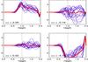 |
Fig. 5 Two horizontal components (top: ℰx, bottom: ℰy) of the turbulence-induced electromotive force for background fields without helicity. Left panels: |

The two horizontal components of the electromotive force are calculated for two different cases. In the first simulation, the applied magnetic fields are assumed to be free of helicity, i.e.  . The other possibility works with
  . If the results of both setups are identical, then the global helicity does not contribute to the electromotive force, as suggested by Eq. (17).
Let us first consider the two different helicity-free cases where, in the y direction, either only a field or only an electric current exists. Hence, for 
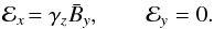 (20)Figure 5 (left) displays the resulting γz as positive (i.e. the flow is downwards) and of order γz ≃ 0.24 in units of cac/ 100 which, with cac ≃ 10 km s-1 approximately1, leads to a downward pumping of 20 m/s. The simulated electromotive force ℰy vanishes as required by (20).
The alternative example with  yields ℰx = 0 and
 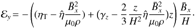 (21)Indeed, the numerically simulated ℰx vanishes while ℰy is negative (see Fig. 5, right).
In Fig. 6 the two components of the electromotive force are shown for a field with global helicity, i.e.  . From (18) one finds
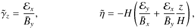 (22)where the tildes mark the magnetically quenched values of the pumping velocity and the eddy diffusivity. The top panels of the plots only concern the advection velocity
  , which is always positive. It sinks from γz ≃ 0.42 to
  for Bx = 10 by the magnetic suppression. From the definition of
  , one immediately finds
  for the quenching coefficient (19) in units of 100H/cac. The code works with ρ0 = 1. We note that in all cases the numerical values of ⟨ u × b ⟩ are very small compared with the scalar product urms and brms given in Fig. 2. The resulting correlation coefficients here are very small.
The existence of an α effect in the expression (17) for the electromotive force would require a term  . No such term resulted from the quasilinear approximation for the influence of helical large-scale fields on nonhelically driven turbulence. This finding can be probed with numerical simulations. We note that three models in Figs. 5 and 6 are computed for constant Bx and for growing helicity (
 , 50, 100). If an α effect existed, we should find that the values of ℰy grow for growing helicity. The numerical results for the three models, however, are always identical. They do not show any numerical response to the growing helicities, which indicates that the nonexistence of an α term that is proportional to
  . The nonexistence of the α term
  in the electromotive force (17) in the quasilinear theory is thusconfirmed by nonlinear simulations.
Equation (22) enables us to derive the magnetic diffusivity from the simulations. By eliminating o from the definitions we find the relation  . With the given mean values for all snapshots, the model with
  provides
  , so that ηT = 0.27 in units of Hcac/ 100 for the unquenched eddy diffusivity. Compared with the traditional estimate ηT ≃ (1 / 3)urmsℓcorr we find the reasonable result ℓcorr ≃ 0.1H in accordance direct inspections of the resulting convection patterns.
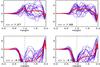 |
Fig. 6 As in Fig. 5, but for the helical background fields with |
3.2. Variation of the magnetic Prandtl number
We still need to verify the analytical formulation (11) after which the ratio of the small-scale current helicity to the large-scale helicity grows with the magnetic Reynolds number. This is certainly only true for large values of Rm (high-conductivity limit). Large Rm require high values of the Reynolds number Re, and/or not too small Pm. It would be more realistic to increase the Reynolds number rather than the magnetic Prandtl number, but Re of order 103 is the upper limit that is allowed by the technical restrictions.
So far the simulations were performed with a fixed magnetic Prandtl number Pm = 0.1. For fixed molecular viscosity its increase (decrease) by one order of magnitude effectively increases (decreases) the magnetic Reynolds number by a factor of ten. We expect a similar reaction of the small-scale current helicity (11). Because of Rm = Pm Re for a fixed Reynolds number, the magnetic Reynolds number runs with Pm.
The results for variations of the magnetic Prandtl number are shown by the plots in Fig. 7. From left to right the magnetic Prandtl number is reduced by a factor of 33. Also the current calculated helicity sinks (by a factor of about 17). The calculated helicity for Pm = 0.1 is 186 (see Fig. 4) and is thus well-situated between the values for Pm = 0.03 and Pm = 1. The current helicity indeed runs with Rm, for which the plots of Fig. 4 in both cases yield values of about 20, which is indeed smaller than the global magnetic Reynolds number of order 100. Also the condition for the high-conductivity limit as the basis of Eq. (11) can be considered as (approximately) fulfilled. Since in Paper I the resulting Rm for weaker fields were much higher, it is possible that, for the present models, the magnetic quenching effect already reduces the numerical values.
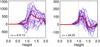 |
Fig. 7 ℋcurr for |

It is easy to verify this statement. It is known that the advection term γz, represented after (20) by  , does not vary with Rm (see Kitchatinov et al. 1994). Hence, we do not expect a similar behavior as in Fig. 7 for the electromotive force ℰx. Indeed, Fig. 8 demonstrates that, for small Rm, the reduction of the magnetic Prandtl number by the factor of 33 leaves the electromotive force ℰx basically unchanged.
The results of Figs. 7 and 8 can also be understood as probing the inner consistency of the models and the numerical procedures. It is also shown that basic results of the quasilinear approximation are confirmed by simulations.
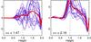 |
Fig. 8 As in Fig. 7 but for ℰx. A similar dependence on the magnetic Prandtl number as in Fig. 7 does not exist. |
4. Conclusions
By analytical (quasilinear) theory and numerical simulations, it is shown that, in a nonrotating convective layer, a large-scale helical magnetic background field produces a small-scale current helicity, while the kinetic helicity vanishes. The current helicity possesses the same sign as the helicity of the large-scale field. The ratio of both pseudoscalars runs with the magnetic Reynolds number of the convection. The same magnetic model provides finite values of the diamagnetic pumping term γ and the eddy diffusivity ηT, but an α effect does not occur in the same order.
If it is true that the α effect in the stellar convection zones is due to the action of the Coriolis force on the turbulent convection, then it is positive (negative) on the northern (southern) hemisphere, which according to Eq. (2) would lead to the opposite signs for the small-scale current helicity – as is indeed observed as dominating during the activity cycle. The new effect of the small-scale current helicity that is due to the influence of a large-scale field combined with a parallel electric current yields opposite signs. During the minimum phase of the solar activity cycle only these signs sometimes occur. Zhang et al. (2010) give
the approximative value 10-5 G2/cm for the observed small-scale current helicity. With the radial scale of 100 Mm and with  G2, one only needs a magnetic Reynolds number Rm of the fluctuations of order 10 to fulfill the numerical constraints.
Numerical values in physical units are always given for the top of the unstable zone.
References
- Abramenko, V. I., Wang, T., & Yurichishin, V. B. 1996, Sol. Phys., 168, 75 [Google Scholar]
- Bao, S., & Zhang, H. 1998, ApJ, 496, L43 [Google Scholar]
- Bhat, P., Blackman, E. G., & Subramanian, K. 2014, MNRAS, 438, 2954 [NASA ADS] [CrossRef] [Google Scholar]
- Blackman, E. G., & Brandenburg, A. 2002, ApJ, 579, 359 [Google Scholar]
- Blackman, E. G., & Subramanian, K. 2013, MNRAS, 429, 1398 [NASA ADS] [CrossRef] [Google Scholar]
- Brandenburg, A., & Subramanian, K. 2005, Phys. Rep., 417, 1 [NASA ADS] [CrossRef] [Google Scholar]
- Bräuer, H. J., & Krause, F. 1974, Astron. Nachr., 295, 223 [NASA ADS] [CrossRef] [Google Scholar]
- Hale, G. E. 1927, Nature, 119, 708 [NASA ADS] [CrossRef] [Google Scholar]
- Keinigs, R. K. 1983,Phys. Fluids, 76, 2558 [Google Scholar]
- Kitchatinov, L. L., Pipin, V. V., & Rüdiger, G. 1994, Astron. Nachr., 315, 157 [NASA ADS] [CrossRef] [Google Scholar]
- Kleeorin, N., Kuzanyan, K., Moss, D., et al. 2003, A&A, 409, 1097 [NASA ADS] [CrossRef] [EDP Sciences] [Google Scholar]
- Pevtsov, A. A., Canfield, R. C., & Latushko, S. M. 2001, ApJ, 549, L261 [NASA ADS] [CrossRef] [Google Scholar]
- Pouquet, A., & Patterson, G. S. 1978, J. Fluid Mech., 85, 305 [NASA ADS] [CrossRef] [Google Scholar]
- Rust, D. M., & Kumar, A. 1994, Sol. Phys., 155, 69 [NASA ADS] [CrossRef] [Google Scholar]
- Rüdiger, G. 1975, Astron. Nachr., 296, 133 [NASA ADS] [CrossRef] [Google Scholar]
- Rüdiger, G., & Kitchatinov, L. L. 1997, Astron. Nachr., 318, 273 [NASA ADS] [CrossRef] [Google Scholar]
- Rüdiger, G., Küker, M., & Schnerr, R. S. 2012, A&A, 546, A23 [NASA ADS] [CrossRef] [EDP Sciences] [Google Scholar]
- Rüdiger, G., Kitchatinov, L. L., & Hollerbach, R. 2013, Magnetic processes in astrophysics: theory, simulations, experiments (Weinheim: Wiley-VCH) [Google Scholar]
- Seehafer, N. 1990, Sol. Phys., 125, 219 [NASA ADS] [CrossRef] [Google Scholar]
- Seehafer, N. 1996, Phys. Rev. E, 53, 1283 [Google Scholar]
- Steenbeck, M., & Krause, F. 1969, Astron. Nachr., 291, 271 [Google Scholar]
- Yousef, T., Brandenburg, A., & Rüdiger, G. 2003, A&A, 411, 321 [NASA ADS] [CrossRef] [EDP Sciences] [Google Scholar]
- Zhang, H. 2012, MNRAS, 419, 799 [NASA ADS] [CrossRef] [Google Scholar]
- Zhang, H., Sakurai, T., Pevtsov, A., et al. 2010, MNRAS, 402, 30 [NASA ADS] [CrossRef] [Google Scholar]
- Ziegler, U. 2004, Comp. Phys. Commun., 157, 207 [NASA ADS] [CrossRef] [Google Scholar]
All Figures
|
Fig. 1 Snapshots of temperature (red lines) and density (blue lines) during the run for |
| In the text | |
|
Fig. 2 Turbulence-intensities |
| In the text | |
|
Fig. 3 As in Fig. 2, but for the correlation coefficients ckin (left) and ccurr (right). The numbers below the graphs are the volume averages of the coefficients over the whole convective domain. The average of all snapshots in both cases is below unity. |
| In the text | |
|
Fig. 4 Small-scale current helicity ⟨ b·curl b ⟩ the result of the large-scale current helicity |
| In the text | |
|
Fig. 5 Two horizontal components (top: ℰx, bottom: ℰy) of the turbulence-induced electromotive force for background fields without helicity. Left panels: |
| In the text | |
|
Fig. 6 As in Fig. 5, but for the helical background fields with |
| In the text | |
|
Fig. 7 ℋcurr for |
| In the text | |
|
Fig. 8 As in Fig. 7 but for ℰx. A similar dependence on the magnetic Prandtl number as in Fig. 7 does not exist. |
| In the text | |
Current usage metrics show cumulative count of Article Views (full-text article views including HTML views, PDF and ePub downloads, according to the available data) and Abstracts Views on Vision4Press platform.
Data correspond to usage on the plateform after 2015. The current usage metrics is available 48-96 hours after online publication and is updated daily on week days.
Initial download of the metrics may take a while.