| Issue |
A&A
Volume 592, August 2016
|
|
|---|---|---|
| Article Number | A106 | |
| Number of page(s) | 4 | |
| Section | The Sun | |
| DOI | https://doi.org/10.1051/0004-6361/201526971 | |
| Published online | 08 August 2016 | |
Verification of the helioseismic Fourier-Legendre analysis for meridional flow measurements
1 Kiepenheuer-Institut für Sonnenphysik, Schöneckstr. 6, 79104 Freiburg, Germany
e-mail: This email address is being protected from spambots. You need JavaScript enabled to view it.
2 Hansen Experimental Physics Laboratory, Stanford University, Standord, CA 94305, USA
e-mail: This email address is being protected from spambots. You need JavaScript enabled to view it.
Received: 16 July 2015
Accepted: 6 March 2016
Abstract
Context. Measuring the Sun’s internal meridional flow is one of the key issues of helioseismology. Using the Fourier-Legendre analysis is a technique for addressing this problem.
Aims. We validate this technique with the help of artificial helioseismic data.
Methods. The analysed data set was obtained by numerically simulating the effect of the meridional flow on the seismic wave field in the full volume of the Sun. In this way, a 51.2-h long time series was generated. The resulting surface velocity field is then analyzed in various settings: Two 360° × 90° halfspheres, two 120° × 60° patches on the front and farside of the Sun (North and South, respectively) and two 120° × 60° patches on the northern and southern frontside only. We compare two possible measurement setups: observations from Earth and from an additional spacecraft on the solar farside, and observations from Earth only, in which case the full information of the global solar oscillation wave field was available.
Results. We find that, with decreasing observing area, the accessible depth range decreases: the 360° × 90° view allows us to probe the meridional flow almost to the bottom of the convection zone, while the 120° × 60° view means only the outer layers can be probed.
Conclusions. These results confirm the validity of the Fourier-Legendre analysis technique for helioseismology of the meridional flow. Furthermore these flows are of special interest for missions like Solar Orbiter that promises to complement standard helioseismic measurements from the solar nearside with farside observations.
Key words: Sun: helioseismology / methods: data analysis / Sun: oscillations / Sun: interior
Now at: Max-Planck-Institut für Sonnensystemforschung, Justus-von-Liebig-Weg 3, 37077 Göttingen, Germany.
Now at: Bay Area Environmental Research Institute, NASA Ames Research Center, Moffett Field, CA 94035, USA.
© ESO, 2016
 Open Access article, published by EDP Sciences, under the terms of the Creative Commons Attribution License (http://creativecommons.org/licenses/by/4.0), which permits unrestricted use, distribution, and reproduction in any medium, provided the original work is properly cited.
1. Introduction
Determining the Sun’s internal meridional flow is one of the main challenges of solar physics. While the meridional flow amplitude at the solar surface is rather easy to measure from feature tracking (Wöhl & Brajša 2001; Hathaway 1996) and the established local helioseismic methods allow us to probe for the flow in shallow sub-surface layers (Haber et al. 2002; Zhao & Kosovichev 2004; González Hernández et al. 2010), a significantly deeper helioseismic probing of the flow encounters difficulties. Since better knowledge about the structure of the meridional flow is desirable for input in to flux-transport dynamo models (Charbonneau 2010), which are essential for understanding the Sun’s magnetic activity cycle, it is the deep meridional flow that is of particular importance. Only recently, improved techniques of time-distance helioseismology (Zhao et al. 2013) and a new approach of global helioseismology (Schad et al. 2013) have provided first indications of the structure of the deep meridional flow. However, today’s helioseismic techniques rely on observations of the frontside of the Sun only. Within the coming years, this type of data might be complemented by missions like the Solar Orbiter, which provides seismic data from the solar farside.
In this paper we focus on inferring the Sun’s internal meridional flow by using the Fourier-Legendre decomposition (FLD) analysis, which is a further development of the concept proposed by Braun & Fan (1998). We employ numerical simulations to create artificial helioseismic data. These data are used to validate the FLD technique and to assess the accuracy of inferences that could be expected from different observational setups.
The paper is organized as follows: Sect. 2 describes the numerical simulations, including the flow model and the Fourier-Legendre technique as it is applied to various observational settings; Sect. 3 presents the results; the conclusions are given in Sect. 4.
2. Methods
Our study rests on analysing artificial helioseismic data, i.e. a time series of a numerically obtained wavefield in the interior of the Sun, which is affected by a large-scale meridional flow.
2.1. Numerical simulation
The generation of artificial helioseismic data is identical to the method described in Hartlep et al. (2013), which makes use of a numerical code that solves the linearized propagation of helioseismic waves throughout the entire solar interior (Hartlep & Mansour 2005). This code has been used in previous studies to simulate the effects of various localized sound-speed perturbations, e.g. for testing helioseismic farside imaging by simulating the effects of model sunspots on the acoustic field (Hartlep et al. 2008; Ilonidis et al. 2009), for validating time -distance helioseismic measurements of tachocline perturbations (Zhao et al. 2009), and for studying the effect of localized subsurface perturbations (Hartlep et al. 2011).
As described in Hartlep et al. (2013), the code has been extended to include the effects of mass flows onto the propagation of helioseismic waves. In short, the code models solar acoustic oscillations in a spherical domain by using the Euler equations that are linearized around a stationary background state. As can be seen in Hartlep et al. (2013), the equations are formulated in a non-rotating frame, and so rotation is accounted for by prescribing an appropriate flow. This approach saves computing the usual Coriolis and centrifugal forces that appear in the equations for a rotating frame.
The excitation of acoustic waves, which is a non-linear process, is not included in the linearized equations. Instead, we mimic solar acoustic wave excitation by including in the momentum equation a random function that is only non-zero close to the solar surface. Perturbations of the gravitational potential have been neglected and the adiabatic approximation has been used. We only consider waves with constant entropy. This way, the entropy gradient of the background model does not enter our equations and the model becomes convectively stable. Non-reflecting boundary conditions are applied at the upper boundary by means of an absorbing buffer layer with a damping coefficient that is zero in the interior and increases smoothly into the buffer layer. A small amount of viscous damping was added for stability reasons.
The simulation in this study resolves spherical harmonics of angular degree between 0 to 170. A staggered Yee scheme (Yee 1966) is used for time integration, with a time step of one second.
2.2. Flow model
For the background flow, we have imposed a stationary model of the solar meridional circulation according to Hartlep et al. (2013). The flow model described there is based on the flow model in Rempel (2006). The meridional flow is a single-cell circulation in each of the meridional quadrants. As described in Hartlep et al. (2013), the amplitude was chosen so that the resulting meridional flow has a maximum velocity of 500 m/s.
But, since these simulations are linear, this kind of an increase does not change the physics but merely increases the signal-to-noise ratio. Hence, a simulated time series of 51.2 h length has the same signal-to-noise ratio as a 3.65 yr-long time series with realistic speeds.
2.3. Fourier-Legendre decomposition
The FLD method is the extension to spherical geometry of the Fourier-Hankel decomposition (FHD) which has been used in the past to study wave absorption in sunspots (Braun et al. 1988). It is a helioseismic technique that is also suited for the measurement of the meridional flow (Braun & Fan 1998). Because the FLD method is sensitive to low-degree oscillation modes, it promises probing the average meridional flow in deep layers. An early version of this FLD analysis pipeline was tested on GONG (Global Oscillation Network Group) data by Doerr et al. (2010), who successfully compared near-surface measurements of the meridional flow with results obtained by ring-diagram analyis.
The time dependent, two-dimensional oscillation signal on the solar surface V(θ,φ,t) can be expressed in terms of a superposition of two wavefields travelling pole- and equatorwards, respectively: ![Mathematical equation: \begin{equation} V(\theta,\phi,t)=\sum_{nlm} \left[A_{lm}H_m^{(1)}(L\theta)+B_{lm}H_m^{(2)}(L\theta)\right]{\rm e}^{{\rm i}m\phi+\omega_{nl}t} \end{equation}](/articles/aa/full_html/2016/08/aa26971-15/aa26971-15-eq6.png) (1)with values of m ≈ 0. Here θ denotes the co-latitude and φ the longitude on the solar surface, ωnl is the angular frequency of a mode with harmonic degree l, L = [l(l + 1)] 1 / 2, and azimuthal order m. The quantitities
(1)with values of m ≈ 0. Here θ denotes the co-latitude and φ the longitude on the solar surface, ωnl is the angular frequency of a mode with harmonic degree l, L = [l(l + 1)] 1 / 2, and azimuthal order m. The quantitities  are travelling wave associated Legendre functions, described in analogy to Nussenzveig (1965):
![Mathematical equation: \begin{equation} H_{m}^{(1,2)}(L\theta) = (-1)^m \frac{(l-m)!}{(l+m)!}\left[P_l^m(\cos\theta) \pm \frac{2\rm i}{\pi}Q_l^m(\cos\theta)\right] , \end{equation}](/articles/aa/full_html/2016/08/aa26971-15/aa26971-15-eq15.png) (2)where
(2)where  and
and  are associated Legendre functions of first and second kind, respectively.
Due to advection, a meridional flow will result in a frequency shift Δνnl between the poleward and equatorward components (Braun & Fan 1998; Gough & Toomre 1983)  (3)where
  is the averaged meridional flow over the observed region of interest as a function of the position r inside the Sun. The sensitivity kernel Knl(r) is the kinetic energy density of a given mode (n,l) which is also a function of the position r inside the Sun.
This frequency shift Δνnl can be measured from the power spectra of the two series, Alm and Blm, by fitting asymmetric Lorentzian profiles to the individual peaks present. The guess frequencies for the fits are obtained from the standard solar Model S (Christensen-Dalsgaard et al. 1996). We then employ the SOLA (subtractive optimally localized averages) inversion technique (Pijpers & Thompson 1994) to construct localized average inversion kernels at a given depth r.
2.4. Data analysis
The simulation results have been tracked with the mean rotation, i.e. transformed to a corotating reference frame with the mean rotation period. The surface velocity field was projected on a heliographic grid and the region of interest is cut out. We study three different observational scenarios:
- 1.
The northern and southern hemispheres, i.e. two patches withangular dimensions of360° × 90° in longitude and latitude, respectively. This corresponds to an ideal observational setup, where data from the whole solar surface is available for helioseismic analysis.
- 2.
Four patches, each with the dimensions 120° × 60°. Two of the patches are on the northern and southern frontside, and two are 180° in longitude apart on the farside, respectively. The patches are centred at ± 35° latitude, respectively. This corresponds to combined observations in the ecliptic from, e.g. Earth and from a spacecraft on the farside of the Sun, as might be possible with missions like the Solar Orbiter (Müller et al. 2013; Roth 2007).
- 3.
Two patches on the frontside only, with the dimensions 120° × 60°. The patches are located at ± 35° latitude. This setup corresponds to the standard case of today’s helioseismic observations with one viewpoint only.
 and
and  of north- and southwards travelling waves are generated for each hemisphere, respectively. These power spectra are then averaged over the range of azimuthal orders m = −25,...,25. This is meant to include a sufficient number of modes that are affected by the meridional flow, as they have a pole- or equatorward directed component of the wave vector. Then, the m-averaged power spectra are smoothed by applying a running boxcar window over three frequency bins. The peaks in the averaged power spectra are then fitted using asymmetric Lorentzian profiles to determine the individual central mode frequencies
  and
and  . Finally, frequency differences
  are calculated. The set of frequency differences is then inverted for the meridional flow, as described above.
3. Results
3.1. Meridional flow measurements
Figure 1 displays the main results of this study. In the first case, where both hemispheres of the Sun could be observed, the input meridional flow can be well recovered (Fig. 1 (top)) down to a depth of 110 Mm. This case corresponds to an ideal observational setup, i.e. the oscillation signal is available for the full solar globe.
In the second case, where only part of the solar surface could be observed, i.e. two patches per hemisphere, one on the front- the other on the farside of the Sun, the flow could still be recovered well. The inversion result agrees well with the input model down to about 30 Mm below the solar surface. Below that, the inversion result deviates significantly from the input flow.
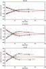 |
Fig. 1 Inversion results for the three observational setups. First row: meridional flow measurements with both hemispheres of the Sun being observed. Second row: same as top, but with two patches for each hemisphere observed on the front and on the farside of the Sun. Third row: same as top but with observations of two patches, one on the northern, the other on the southern hemisphere. The red lines indicate the averaged flow amplitudes below the observed patches on the northern and southern hemispheres, as taken from the input model. Horizontal error bars represent the quantile width of the averaging kernels. |
In the third case, where only frontside observations are available, the flow can be reliably recovered down to only 30 Mm, too. At deeper layers the inversion results deviate strongly from the input flow.
We note that, since the numerical data included only low degree modes, the surface flow was not recovered in all settings. The flow measurements were possible at depths greater than 10 Mm.
3.2. Power leaks
According to theoretical forward calculations by Roth & Stix (2008) and Gough & Hindman (2010), the frequency shifts introduced by a meridional flow should be negligible. Given the results by Gough & Hindman (2010), the meridional flow should introduce a power redistribution among affected modes. In fact, this power redistribution comes from the coupling of modes owing to advection, which affects the eigenfunctions (Lavely & Ritzwoller 1992; Schad et al. 2011). This is an effect that is evaluated in global helioseismology to measure the meridional flow (Schad et al. 2013).
Nevertheless, in this study, we successfully make us of measurable frequency shifts. By studying the power spectra of pole- and equatorwards travelling waves in detail, it becomes obvious that the modes are actually not measurably shifted and that this frequency shift must be spurious. Two effects need to be considered. First, due to the fact that only parts of the solar surface are used for Fourier-Legendre decomposition, the spherical harmonics are no longer orthogonal on these reduced areas of the solar surface. As a result, spatial leaks appear. Figure 2 shows the power spectra for our three observational setups. As visible in Fig. 2, this number of leaks increases with decreasing observing area, i.e. the central peak amplitude decreases and power leaks into a broad range of side lobes. Second, the coupling of modes, which are caused by advection, introduces a number of side lobes i.e. power leaks, in the mode spectra, too. By comparing pole- and equatorward propagating waves, it can be seen that the individual central mode peak and its leaks do not change their position on the frequency axis. But, owing to the presence of the meridional flow, power is redistributed among the leaks in a way that the weight of the whole set of coupled modes is shifted in frequency. Consequently, smoothing the power spectra over frequency and fitting a common asymmetric Lorentzian profile to the resulting broad peak must yield shifted frequencies. This apparent frequency difference between pole- and equatorward travelling waves can then be employed for inversions. Making use of the mode kinetic energy, however, needs to be considered as an approximation to proper sensitivity kernels, which are not yet available for this technique.
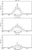 |
Fig. 2 Exemplary power spectra averaged over azimuthal orders m = −25,...,25 for the poleward (solid) and equatorward (dashed) travelling waves with harmonic degree l = 90 and radial order n = 7. From top to bottom, the viewing area decreases from 360° × 90°, over 2 × 120° × 60°, to 120° × 60°. Power is normalized with the same factor in all three plots. |
4. Conclusion
We have validated the Fourier-Legendre decomposition technique as a means of measuring the meridional flow. For this we employed artificial helioseismic data. The technique was applied to three settings that mimic observation scenarios. These range from ideal conditions of full surface observations of the oscillation signal to the grade of scenarios, which are more compatible with observations that are technically possible today, i.e. observing parts of the solar hemisphere on the front- and farside only.
As a main result, we were able to demonstrate that the technique successfully recovers the meridional flow that was included in the simulation. This works better when more of the solar surface is available for helioseismic analysis. We conclude that in the case that one hemisphere can be fully observed, a meridional flow within of 20 m/s amplitude could be inferred by a 3.65-yr long time series with this technique, if the results from the 51.2 h of artificial data are comparable to 3.65 yrs of observational data, which is not, a priori, clear, especially as helioseismic techniques work very well on simulations that are linear or convectively stable. More advanced simulations should therefore be considered in future for testing this technique, too.
We note that the technique makes use of an apparent frequency shift, which comes from the fact that power is redistributed between modes that are coupled by the meridional flow. This creates asymmetric weights in the power distribution of a mode and its leaks that are close-by in frequency, which can be interpreted as a frequency shift. Therefore, we can confirm the theoretical results obtained by Gough & Hindman (2010), but are still able to use the technique to measure the meridional flow down to great depths. This works as long as the individual power leaks are not resolved in frequency because then the mode kinetic energy can serve as an approximation of the proper sensitivity kernels for this technique. The derivation of these kernels would be part of a future study. Thus, making use of the power redistribution would therefore be the next step in developing this technique further because, accounting for the leakage of modes promises a better recovery of the flow at greater depths. As a consequence, the results of the FLD analysis will be more comparable to other methods, e.g. time-distance helioseismology. For example, Jackiewicz et al. (2015) analyze this simulation too, using the time-distance technique and obtain more accurate inversion results in deeper layers. Still, the method promises advantages in its capability of easy incorporation of data from multiple vantage points, which is a result from the applicability of the method to various patch geometries, in contrast to the ring-diagram technique.
Concerning multiple vantage points, we conclude that the meridional flow could be detected down to a large percentage of the convection zone using the Fourier-Legendre analysis technique when observational data from front- and farside observations are combined. Therefore our study may be interesting when planning upcoming space missions, e.g. Solar Orbiter.
Acknowledgments
M.R. thanks D. Braun for useful discussions. The authors thank the unknown referee for valuable comments on the manuscript. The research leading to these results has received funding from the European Research Council under the European Union’s Seventh Framework Program (FP/2007-2013)/ERC Grant Agreement No. 307117.
References
- Braun, D. C., & Fan, Y. 1998, ApJ, 508, L105 [NASA ADS] [CrossRef] [Google Scholar]
- Braun, D. C., Duvall, Jr., T. L., & Labonte, B. J. 1988, ApJ, 335, 1015 [NASA ADS] [CrossRef] [Google Scholar]
- Charbonneau, P. 2010, Liv. Rev. Sol. Phys., 7, 3 [Google Scholar]
- Christensen-Dalsgaard, J., Dappen, W., Ajukov, S. V., et al. 1996, Science, 272, 1286 [CrossRef] [Google Scholar]
- Doerr, H.-P., Roth, M., Zaatri, A., Krieger, L., & Thompson, M. J. 2010, Astron. Nachr., 331, 911 [NASA ADS] [CrossRef] [Google Scholar]
- González Hernández, I., Howe, R., Komm, R., & Hill, F. 2010, ApJ, 713, L16 [NASA ADS] [CrossRef] [Google Scholar]
- Gough, D., & Hindman, B. W. 2010, ApJ, 714, 960 [NASA ADS] [CrossRef] [Google Scholar]
- Gough, D. O., & Toomre, J. 1983, Sol. Phys., 82, 401 [NASA ADS] [CrossRef] [Google Scholar]
- Haber, D. A., Hindman, B. W., Toomre, J., et al. 2002, ApJ, 570, 855 [NASA ADS] [CrossRef] [Google Scholar]
- Hartlep, T., & Mansour, N. N. 2005, Annual Research Briefs, Center for Turbulence Research, NASA Ames/Stanford University [Google Scholar]
- Hartlep, T., Zhao, J., Mansour, N. N., & Kosovichev, A. G. 2008, ApJ, 689, 1373 [NASA ADS] [CrossRef] [Google Scholar]
- Hartlep, T., Kosovichev, A. G., Zhao, J., & Mansour, N. N. 2011, Sol. Phys., 268, 321 [NASA ADS] [CrossRef] [Google Scholar]
- Hartlep, T., Zhao, J., Kosovichev, A. G., & Mansour, N. N. 2013, ApJ, 762, 132 [NASA ADS] [CrossRef] [Google Scholar]
- Hathaway, D. H. 1996, ApJ, 460, 1027 [Google Scholar]
- Ilonidis, S., Zhao, J., & Hartlep, T. 2009, Sol. Phys., 258, 181 [NASA ADS] [CrossRef] [Google Scholar]
- Jackiewicz, J., Serebryanskiy, A., & Kholikov, S. 2015, ApJ, 805, 133 [NASA ADS] [CrossRef] [Google Scholar]
- Lavely, E. M., & Ritzwoller, M. H. 1992, Roy. Soc. London Philos. Trans. Ser. A, 339, 431 [Google Scholar]
- Müller, D., Marsden, R. G., St. Cyr, O. C., & Gilbert, H. R. 2013, Sol. Phys., 285, 25 [NASA ADS] [CrossRef] [Google Scholar]
- Nussenzveig, H. M. 1965, Ann. Phys., 23, 23 [Google Scholar]
- Pijpers, F. P., & Thompson, M. J. 1994, A&A, 281, 231 [NASA ADS] [Google Scholar]
- Rempel, M. 2006, ApJ, 647, 662 [NASA ADS] [CrossRef] [Google Scholar]
- Roth, M. 2007, in Modern solar facilities − advanced solar science, eds. F. Kneer, K. G. Puschmann, & A. D. Wittmann, 85 [Google Scholar]
- Roth, M., & Stix, M. 2008, Sol. Phys., 251, 77 [NASA ADS] [CrossRef] [Google Scholar]
- Schad, A., Timmer, J., & Roth, M. 2011, ApJ, 734, 97 [Google Scholar]
- Schad, A., Timmer, J., & Roth, M. 2013, ApJ, 778, L38 [NASA ADS] [CrossRef] [Google Scholar]
- Wöhl, H., & Brajša, R. 2001, Sol. Phys., 198, 57 [NASA ADS] [CrossRef] [Google Scholar]
- Yee, K. 1966, IEEE Transactions on Antennas and Propagation, 14, 302 [Google Scholar]
- Zhao, J., & Kosovichev, A. G. 2004, ApJ, 603, 776 [NASA ADS] [CrossRef] [Google Scholar]
- Zhao, J., Hartlep, T., Kosovichev, A. G., & Mansour, N. N. 2009, ApJ, 702, 1150 [NASA ADS] [CrossRef] [Google Scholar]
- Zhao, J., Bogart, R. S., Kosovichev, A. G., Duvall, Jr., T. L., & Hartlep, T. 2013, ApJ, 774, L29 [NASA ADS] [CrossRef] [Google Scholar]
All Figures
|
Fig. 1 Inversion results for the three observational setups. First row: meridional flow measurements with both hemispheres of the Sun being observed. Second row: same as top, but with two patches for each hemisphere observed on the front and on the farside of the Sun. Third row: same as top but with observations of two patches, one on the northern, the other on the southern hemisphere. The red lines indicate the averaged flow amplitudes below the observed patches on the northern and southern hemispheres, as taken from the input model. Horizontal error bars represent the quantile width of the averaging kernels. |
| In the text | |
|
Fig. 2 Exemplary power spectra averaged over azimuthal orders m = −25,...,25 for the poleward (solid) and equatorward (dashed) travelling waves with harmonic degree l = 90 and radial order n = 7. From top to bottom, the viewing area decreases from 360° × 90°, over 2 × 120° × 60°, to 120° × 60°. Power is normalized with the same factor in all three plots. |
| In the text | |
Current usage metrics show cumulative count of Article Views (full-text article views including HTML views, PDF and ePub downloads, according to the available data) and Abstracts Views on Vision4Press platform.
Data correspond to usage on the plateform after 2015. The current usage metrics is available 48-96 hours after online publication and is updated daily on week days.
Initial download of the metrics may take a while.