| Issue |
A&A
Volume 591, July 2016
|
|
|---|---|---|
| Article Number | A77 | |
| Number of page(s) | 6 | |
| Section | Stellar structure and evolution | |
| DOI | https://doi.org/10.1051/0004-6361/201628428 | |
| Published online | 20 June 2016 | |
Research Note
Non-linear behaviour of XTE J1550-564 during its 1998−1999 outburst, revealed by recurrence analysis
Center for Theoretical Physics, Polish Academy of Sciences,
Al. Lotnikow 32/46,
02-668
Warsaw,
Poland
e-mail: This email address is being protected from spambots. You need JavaScript enabled to view it.
Received:
3
March
2016
Accepted:
5
May
2016
Abstract
We study the X-ray emission of the microquasar XTE J1550-564 and analyze the properties of its light curves using the recurrence analysis method. The indicators for non-linear dynamics of the accretion flow are found in the very high state and soft state of this source. The significance of deterministic variability depends on the energy band. We discuss the non-linear dynamics of the accretion flow in the context of the disc-corona geometry and propagating oscillations in the accretion flow.
Key words: black hole physics / accretion, accretion disks / chaos
© ESO, 2016
1. Introduction
The microquasar XTE J1550-564 is a low-mass X-ray binary (LMXB), with a companion main sequence star, and was discovered in its 1998 outburst by the All-Sky Monitor onboard the RXTE satellite (Smith et al. 1998). The radio-jets that accompany its activity were also detected, similarly to many other black hole X-ray binaries (Hannikainen et al. 2001). The compact object’s mass is estimated at 8−11 Solar masses and thus it is considered to be a black hole (Orosz et al. 2002). The source exhibits all the canonical spectral states typically associated with LMXBs.
The source’s spectral analysis performed for the RXTE data of XTE J1550-564, that spans the period between September 23 and October 6, 1998, place this object in the very high state (VHS) category (Gierliński & Done 2003). Further analysis performed for this source by Kubota & Done (2004) showed that the temperature of the accretion disk is much lower than expected for the VHS luminosity, and suggested that this should be interpreted as the signature of the disk truncation at the radius of about 30 Rg.
Non-linear dynamics indicator  obtained for Nϵ different values of recurrence threshold ϵ in different energy bands for three observations 30188-06-05-00 (MJD 51 068), 30191-01-12-00 (MJD 51 082) and 30191-01-33-00 (MJD 51 108).
The intrinsic luminosity of the source peaks above 1039 erg/s, and during both very high and soft states it remains well above 2−3 × 1038 erg/s. Therefore the derived accretion rate can be in this source equal to at least 25% of the Eddington limit, and reaching even 0.8 ṀEdd at the outburst peak. In the standard accretion disk theory, such high values of Ṁ lead to the intrinsic thermal and viscous instabilities caused by the dominant radiation pressure. Such instabilities manifest themselves in the non-lienar evolution of the disk temperature and density at very short timescales, and consequently imprint a characteristic, time-dependent pattern in the emitted X-ray luminosity.
In this work, we study the properties of the XTE J1550-564 light curves. We implement our method, recently described in Suková et al. (2016), and we study the light curves in the X-rays as taken by the RXTE satellite during the fall 1998 and spring 1999. The capabilities of this method were tested numerically in Suková & Janiuk (2016) and its dependence on parameters was discussed in Grzedzielski et al. (2015). Here we focus on the spectral and temporal evolution of the microquasars’s properties and its possible non-linear behaviour. We discuss the results in the context of the thermal-viscous instability of a Keplerian accretion disc, as well as coupling of its variability with the behaviour of hard X-ray emitting, quasi-spherical corona.
2. Observational data
The overall light curve and hardness ratio of the outburst of XTE J1550-564 shows two separated stages of high luminosity (Bradt et al. 2000). The first one lasted from the beginning of September to the beginning of October 1998 (MJD 51 063 to 51 120), and the second one spanned from the mid of December 1998 to the mid of April 1999 (MJD 51 160 to 51 280). From the list of the publicly available observations made by RXTE in NASA’s HEASARC arxiv1 we selected several observations, which cover the two epochs quite evenly and which are long enough for our purpose. The data sample is summarised in Table 2.
3. Recurrence analysis and non-linear dynamics indicator
We study the properties of the light curves obtained in different energy bands by means of the time series analysis. Our aim is to find out if the time variability of the flux contains the information about the nature of the dynamical system behind the emission of the radiation. Mainly, we want to discover if the underlying system behaves according to deterministic non-linear dynamics, which is governed by a low number of equations rather than by stochastic variations. In the former case, the traces of the non-linear behaviour are imprinted into the outgoing radiation.
In the preceding paper (Suková et al. 2016) we developed the method, which can reveal such traces hidden in the observational data. The method includes performing recurrence analysis on the observational time series, which is in our case the light curve, and on the set of surrogate data series. The results are then compared according to discriminating statistics. Our null hypothesis is that the data are a product of a linearly autocorrelated Gaussian process, so that the data point is given by a linear combination of the preceding points and a contribution of uncorrelated Gaussian noise, ξ(n), hence 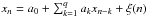 . The properties of such time series are fully described by their Fourier spectrum. The surrogate data are constructed in such a way that they share the value distribution and the Fourier spectrum with the original series (Theiler et al. 1992; Schreiber & Schmitz 2000). However, if the original time series is a product of a non-linear system, the dynamical attributes obtained by the analysis will differ from the surrogate series.
Here we use this method to study the outburst of XTE J1550-564, so we only briefly describe its main points. We normalise the light curve to have zero mean and unit variance, then we construct a bunch of 100 surrogates using the procedure surrogates from TISEAN2 (Hegger et al. 1999).The recurrence analysis is performed on the basis of the software package described by Marwan et al. (2007), Marwan (2013), which also yields the cumulative histogram of diagonal lines.We compute the recurrence quantifiers for the data and the surrogates, using the educated guess of its parameters time delay Δt and embedding dimension m for a set of recurrence thresholds ϵ, such that the recurrence rate is approximately in the range (1%−25%).
After computing the cumulative histograms of diagonal lines for the observed data and their surrogates, we estimate the Rényi’s entropy K2 by the linear regression of the cumulative histogram. We follow the rules given in Suková et al. (2016) Appendix B, in particular that the minimal length of the diagonal lines must exceed the time delay and that there must be at least five points for the regression.
As the discriminating statistic we choose the logarithm of the estimated Rényi’s entropy, which we compute for each threshold for the observed time series  and similarly for the set of surrogates
  . We find the mean
  and the standard deviation
  of the set . Then we define the weighted significance as
 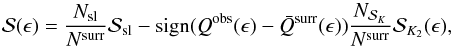 (1)where Nsl is the number of surrogates, which have only short diagonal lines, and Nsurr is the total number of surrogates,
  and
and  is the significance computed only from the surrogates, which have enough long lines according to the relation
 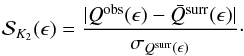 (2)Finally, we define the non-linear dynamics (NLD) indicator, , as the average of
  over the set of Nϵ different thresholds. We say that the observation shows traces of non-linear behaviour if it exceeds the chosen threshold,
  .
.
The accuracy of the resulting NLD indicator is quite a complicated issue, because the observational data with their uncertainness undergo several subsequent statistical processes. However, we can treat the resulting values as a small set of Nϵ measurements of . As such, the uncertainty of NLD indicator is given as  , where R is the spread of the data set, that is
  .
.
4. Results
4.1. Energy dependence of NLD indicator
We start our study with the observation 30188-06-05-00 taken on 12.9.1998 (MJD 51 068). We extract the data with the time bin dt = 0.025s in six energy bands denoted as A − F, which are listed in Table 1. We take the longest available continuous part of the light curve up to Nmax = 32 768 points. We set the upper limit of the length of the studied time series in order to keep the numerical demands to a reasonable level. The light curve in band F, the recurrence plot (RP)3 of the observation and RP of one of the surrogates are plotted in Fig. 1.
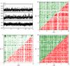 |
Fig. 1 Lightcurves in energy band F and recurrence plots for the observations (in red) and one surrogate (in green) for the three observations listed in Table 1: a) MJD 51 068 b) MJD 51 082 c) MJD 51 108. |
We compute the NLD indicator with the parameters m = 9 and k = 4. The highest is obtained for the energy band D, which covers the energy range 7.96−12.99 keV. On the other hand in the lowest energy band A, the NLD indicator is very small ( ).
).
The indicator increases from band A to band D, slightly exceeding our threshold in band B ( ) and giving quite a high value
  in band C. In the highest energies covered by band E, the value decreases to
  .
.
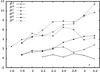 |
Fig. 2 Dependence of |

Observations selected for the analysis.
We also provide results for the energy band F, which includes channels 0−35 (<12.99 keV). This band corresponds to the extraction of the data from the binned mode or the single-bit mode without energy filtering, so that such a light curve has the highest count rate. This band can also be compared with the results given in Suková et al. (2016). The light curve in this band yields a high value 
We notice that the uncertainty σ of NLD given in Table 1 in bands D and F is very high. The reason for this is that the significance is not independent on ϵ, but rather grows with the threshold and the spread of the data set is high (see Fig. 2). This behaviour is not so prominent in any other case, and can be explained if the underlying cumulative histograms are inspected.
The histograms of this observation for higher thresholds show an “elbow” around l ~ 3.5 s and the slope of the part after the elbow is about two times smaller than for the shorter lines. A similar elbow is not seen in the histograms of the surrogates, partly because they do not have many such long lines. For higher ϵ, the elbow is more prominent in the observation’s histogram, lowering the estimated value of  and thus making the difference between the observation and the surrogates bigger.
This feature can be explained as the presence of recurrence period in the system. The slope of the first part is higher, because it is more difficult to predict the evolution of the trajectory, when we have information about its piece shorter than the recurrence period (see Marwan et al. 2007 for more details about the properties of RPs). Also a possible interplay between the value of the recurrence threshold and the noise in the data can play a role in this effect.
Similar analysis of the energy dependence of NLD was also made for two later observations, 30191-01-12-00 taken on MJD 51 082, and 30191-01-33-00 taken on MJD 51 108 (denoted as b, and c in Fig. 1).
The second observation yields similar values of NLD in bands D and C and the overall band F gives the highest value. The third observation also has its highest significance in the band F, however for this observation the NLD indicator in band C is higher then in band D. The values in all bands are much less than for the first two observations, which suggests that the non-linear dynamics in the source fades away during the outburst.
4.2. Temporal evolution of NLD indicator during the outburst
We continue with the study of the temporal evolution of the NLD indicator during the outburst of XTE J1550-564. We extract the light curves in energy bands D and F for each observation from Table 2. In order to use our procedure meaningfully, we need to have a sufficiently high number of counts in each time bin. Hence, the total count rate combined from all working proportional counter units (PCUs) in each energy band is an important quantity for setting the time bin dt. We provide the values and the number of working PCUs in Table 2. The normalised count rate per PCU is given in Figs. 3a and b, respectively.
We quantify the hardness ratio as the count rate in band D divided by count rate in lower energies, h = ND/ (NF − ND), which is given in Table 2 and in Fig. 3c. Strong spectral transition from hard state, with h ≳ 0.2, to soft state, with h ≈ 0.05, can be seen during the first stage of the outburst. Hence, the count rate in band D drops down significantly in the later epoch. Therefore we do not compute the significance in band D for observations after 1.11.1998 (MJD 51 119).
During the second stage of the outburst, the hardness ratio h is much lower, with the exception of short time period around MJD 51 250 (see Kubota & Done 2004), when it reaches h = 0.18. We map this time period more closely, choosing several observations between MJD 51 240 and MJD 51 250. Apart from those observations, the count rate in band D is low, so that applying our method on the light curve in band D is not possible due to the lack of counts in a short time bin. Because of this, we provide NLD indicator only for band F.
We use the time bin dtF = 0.032s for light curves in band F and dtD = 0.025s for light curves in band D. We find the educated guess of the embedding dimension m and the time delay Δt = kdt as in Suková et al. (2016). The values vary in the range m ∈ [ 7,9 ] and k ∈ [ 2,9 ]. For each observation and each energy band, Nϵ indicates the number of different ϵ, for which the NLD indicator is obtained by averaging the significance.
Our results, which are summarised in Table 2 and plotted in Fig. 4, show that the NLD indicator is higher in band D than in band F at the beginning of the outburst. This is in agreement with the result obtained for the observation 30188-06-05-00 (see Table 1). The traces of non-linear dynamics are most prominent in the light curves consisting of counts in the energy range of 8−13 keV. Hence, the non-linear behaviour of the accreting system is expected to manifest mainly in the regions that emit radiation in energies 8−13 keV.
Later, this tendency is smeared and  in some cases. The non-linear behaviour shifts into lower energies as the outburst continues, while its total importance decreases. This supports the trend, which we presented in Sect. 4.1 for the three selected observations.
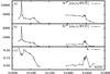 |
Fig. 3 Characteristics of the source XTE J1550-564 during both epochs of the outburst 1998/1999. a) Count rate in energy band F. b) Count rate in energy band D. c) Hardness ratio h. |
 |
Fig. 4 NLD indicator in band D and F during the outburst of XTE J1550-564. The threshold 1.5 for significant result is indicated by the dashed horizontal line. |
The obvious exception of the NLD indicator behaviour is the observation 30191-01-02-00, taken on MJD 51 075, for which the NLD indicator in band F is slightly above the threshold, but the NLD indicator in band D is non-significant. This observation is special because it covers the peak of the outburst, during which the count rate is three times higher than in any other observation. Remarkably, the hardness ratio does not vary much, having very similar value, h = 0.21, like for the other observations.
On MJD 51 110, the NLD indicator is less than one in both bands and the evidence for non-linear behaviour vanishes. The hardness ratio drops down to h = 0.13, while the total count rate NF remains at similar level ~14 000 cts/s. From that moment, not only the hardness ratio decreases further to h ~ 0.05, but the total count rate also declines significantly. NLD indicator shows no signs of non-linear dynamics.
After the source stays at a low luminosity level for about two months, the second stage of the outburst occurs. This epoch spans approximately from the middle of January to the beginning of April 1999.
During this epoch, the count rate in band F reaches similar values to the first stage (~15 000 cts/s) except for the outburst peak. Almost all observations from this stage including those with higher h provide non-significant values of NLD indicator, with only slight glimpses of non-linear motion on MJD 51 245 ( ) and MJD 51 247 (
 ). Hence, there are only very weak signs of non-linear dynamics during the second epoch of the outburst and the behaviour of the source is considerably different from the first stage.
5. Discussion
During the two epochs of the outburst the source XTE J1550-564 undergoes a complicated evolution of its total luminosity and the spectral and timing properties. Existence and properties of quasi-periodic oscillations (QPOs) were studied, for example, by Remillard et al. (2002), Sobczak et al. (2000b), Heil et al. (2011). Detailed spectral study was provided by Sobczak et al. (2000a).
Kubota & Done (2004) discussed the spectral fitting of the data with respect to the geometry of the accretion flow. They focus on the first epoch of the outburst, when the evolution goes from a low/hard state through a strong very high state, VHS and a weak VHS to the standard high/soft state. Authors show that the data are hardly compatible with the constant inner radius of the accretion disc. They propose a scenario of the evolution of the accretion flow during the initial state of the outburst, which involves the accretion disc truncated at higher radius than the ISCO, which is immersed in the hot Comptonizing corona. With the elapsed time, the disc propagates closer to the center, eventually reaching the ISCO around MJD 51 105. Within next 12 days the remaining corona disappears and the source moves into the standard high/soft state.
The connection of the outburst time and spectral variability with the properties of companion star was shown by Wu et al. (2002). They proposed a scenario of the outburst, which begins with the accretion of low angular momentum gas released from a magnetic trap near the L1 point created by the companion star magnetic field. At the same time high angular momentum accretion also begins through the Roche lobe overflow forming an accretion disc further away. However, the low angular momentum accretion is much faster, operating near the free fall speed, and the electrons gains high energy. Close to the black hole, where a centrifugal barrier is met, a shock in this component could create and possibly oscillate, showing the non-linear behaviour and radiating in the highest energies. This scenario explains the fast rise of the hard X-ray component versus much slower rise of the soft component, and it is compatible with the previously presented picture of the colder Keplerian disc slowly propagating inward through the already existing hot corona (Kubota & Done 2004).
This scenario is also viable in point of view of our results. We showed that at the beginning of the outburst the non-linear behaviour is the strongest in the higher energies, particularly in band D. We note that the drop down of the NLD indicator in the highest energy band E may be caused by a small count rate, and perhaps data from different instrument would be more suitable for the analysis in the highest energies. Later the non-linear dynamics is more prominent in lower energies (band C).
The oscillations of the accretion disc caused by the radiation pressure instability occurs typically on timescales of at least five to ten seconds. The exact value depends on the global parameters of the source, such as the black hole mass and viscosity in the accretion disk, and is triggered by the accretion rate being a large fraction of the Eddington. The threshold accretion rate for the instability depends weakly on the system parameters. The truncation of the inner disc, on the other hand, could shut down the instability in XTE J1550-564. For instance, the disc truncated at 30 Schwarzschild radii would be completely stable, if the accretion rate is below 0.7 of Eddington rate. Therefore only the “memory” of the disc’s oscillations would be kept in the hot corona, which is dynamically and radiatively coupled with the disc. It should also be noted, that instead of the regular outbursts on large amplitudes and long timescales, which are not observed in XTE J1550-564, a kind of flickering behaviour is possible, in case of a specific configuration of system parameters for which the disc is only marginally unstable (Grzedzielski et al., in prep.).
Here, we link the non-linear behaviour of the high energy emitting regions with the oscillations inside the corona, triggered by the formation and propagation of the accretion disc in the equatorial plane. When the disc is more deeply immersed in the corona, the non-linear behaviour shifts to the lower energies. When the disc reaches the ISCO, and accretion rate is low, it stabilises and emits only thermal stochastic radiation. The oscillations of the corona cease and the corona itself is depleted within several days.
The propagation of oscillations through the corona can potentially lead to the evolution of the low frequency QPOs, modelled by Chakrabarti et al. (2009) within an outburst scenario, that invoked formation of a shock in the inner region. We can expect that during the flare peak (MJD 51 075) any non-linear oscillatory behaviour is overpowered by some rapid, very energetic event accompanied by a strong stochastic emission, so that the NLD indicator is quite low. This can be related to the jet launching because strong radio emission, which peaked two days after the X-rays, was observed preceded by a peak in optical band that occurred about one day after the X-ray peak (Wu et al. 2002). A few days later the apparent superluminal motion of the ejecta in the radio band was observed (Hannikainen et al. 2001).
In the second epoch of the outburst, we detect no strong signs of non-linear behaviour, even in the short period between MJD 51 244 and MJD 51 250, when the hardness ratio increased significantly. Here, however, the overall evolution of the source is different. We first see the soft state with high luminosity and small h, compatible with an accretion disc spanned down to the ISCO, and then the increase of the high energy flux ND (and h). Obviously, the mechanism of the corona creation in this case is different than in the first epoch and the non-linear mechanism leading to the oscillations is not triggered.
heasarc.gsfc.nasa.gov
Recurrence plot is a visualisation of the recurrence matrix, where the recurrence points are plotted as dots. Because the plot is symmetric with respect to the main diagonal, we plot only the triangle below/above the diagonal.
Acknowledgments
This work was supported in part by the grant DEC-2012/05/E/ST9/03914 from the Polish National Science Center.
References
- Bradt, H., Levine, A. M., Remillard, R. A., & Smith, D. A. 2000, ArXiv e-prints [arXiv:astro-ph/0001460] [Google Scholar]
- Chakrabarti, S. K., Dutta, B. G., & Pal, P. S. 2009, MNRAS, 394, 1463 [NASA ADS] [CrossRef] [Google Scholar]
- Gierliński, M., & Done, C. 2003, MNRAS, 342, 1083 [NASA ADS] [CrossRef] [Google Scholar]
- Grzedzielski, M., Sukova, P., & Janiuk, A. 2015, JA&A, 36, 529 [NASA ADS] [Google Scholar]
- Hannikainen, D., Campbell-Wilson, D., Hunstead, R., et al. 2001, Astrophys. Space Sci., 276, 45 [CrossRef] [Google Scholar]
- Hegger, R., Kantz, H., & Schreiber, T. 1999, Chaos: An Interdisciplinary Journal of Nonlinear Science, 9, 413 [NASA ADS] [CrossRef] [PubMed] [Google Scholar]
- Heil, L. M., Vaughan, S., & Uttley, P. 2011, MNRAS, 411, L66 [NASA ADS] [CrossRef] [Google Scholar]
- Kubota, A., & Done, C. 2004, MNRAS, 353, 980 [NASA ADS] [CrossRef] [Google Scholar]
- Marwan, N. 2013, Commandline Recurrence Plots, http://tocsy.pik-potsdam.de/commandline-rp.php, accessed: 2015-07-21 [Google Scholar]
- Marwan, N., CarmenRomano, M., Thiel, M., & Kurths, J. 2007, Phys. Rep., 438, 237 [Google Scholar]
- Orosz, J. A., Groot, P. J., van der Klis, M., et al. 2002, ApJ, 568, 845 [NASA ADS] [CrossRef] [Google Scholar]
- Remillard, R. A., Sobczak, G. J., Muno, M. P., & McClintock, J. E. 2002, ApJ, 564, 962 [Google Scholar]
- Schreiber, T., & Schmitz, A. 2000, Phys. D: Nonl. Phenomena, 142, 346 [Google Scholar]
- Smith, M. J. S., Ricci, R., in ’t Zand, J., et al. 1998, IAU Circ., 6938 [Google Scholar]
- Sobczak, G. J., McClintock, J. E., Remillard, R. A., et al. 2000a, ApJ, 544, 993 [NASA ADS] [CrossRef] [Google Scholar]
- Sobczak, G. J., McClintock, J. E., Remillard, R. A., et al. 2000b, ApJ, 531, 537 [NASA ADS] [CrossRef] [Google Scholar]
- Suková, P., & Janiuk, A. 2016, Workshop series of the Argentinian Astronomical Society, submitted [arXiv:1604.02670] [Google Scholar]
- Suková, P., Grzedzielski, M., & Janiuk, A. 2016, A&A, 586, A143 [NASA ADS] [CrossRef] [EDP Sciences] [Google Scholar]
- Theiler, J., Eubank, S., Longtin, A., Galdrikian, B., & Farmer, J. D. 1992, Phys. D: Nonlin. Phenomena, 58, 77 [Google Scholar]
- Wu, K., Soria, R., Campbell-Wilson, D., et al. 2002, ApJ, 565, 1161 [NASA ADS] [CrossRef] [Google Scholar]
All Tables
Non-linear dynamics indicator obtained for Nϵ different values of recurrence threshold ϵ in different energy bands for three observations 30188-06-05-00 (MJD 51 068), 30191-01-12-00 (MJD 51 082) and 30191-01-33-00 (MJD 51 108).
All Figures
|
Fig. 1 Lightcurves in energy band F and recurrence plots for the observations (in red) and one surrogate (in green) for the three observations listed in Table 1: a) MJD 51 068 b) MJD 51 082 c) MJD 51 108. |
| In the text | |
|
Fig. 2 Dependence of |
| In the text | |
|
Fig. 3 Characteristics of the source XTE J1550-564 during both epochs of the outburst 1998/1999. a) Count rate in energy band F. b) Count rate in energy band D. c) Hardness ratio h. |
| In the text | |
|
Fig. 4 NLD indicator in band D and F during the outburst of XTE J1550-564. The threshold 1.5 for significant result is indicated by the dashed horizontal line. |
| In the text | |
Current usage metrics show cumulative count of Article Views (full-text article views including HTML views, PDF and ePub downloads, according to the available data) and Abstracts Views on Vision4Press platform.
Data correspond to usage on the plateform after 2015. The current usage metrics is available 48-96 hours after online publication and is updated daily on week days.
Initial download of the metrics may take a while.