| Issue |
A&A
Volume 591, July 2016
|
|
|---|---|---|
| Article Number | A100 | |
| Number of page(s) | 22 | |
| Section | Interstellar and circumstellar matter | |
| DOI | https://doi.org/10.1051/0004-6361/201526975 | |
| Published online | 22 June 2016 | |
Formation of H2-He substellar bodies in cold conditions
Gravitational stability of binary mixtures in a phase transition
Geneva Observatory, University of Geneva, 1290 Sauverny, Switzerland
e-mail: andreas.fueglistaler@unige.ch
Received: 16 July 2015
Accepted: 25 March 2016
Context. Molecular clouds typically consist of 3/4 H2, 1/4 He and traces of heavier elements. In an earlier work we showed that at very low temperatures and high densities, H2 can be in a phase transition leading to the formation of ice clumps as large as comets or even planets. However, He has very different chemical properties and no phase transition is expected before H2 in dense interstellar medium conditions. The gravitational stability of fluid mixtures has been studied before, but these studies did not include a phase transition.
Aims. We study the gravitational stability of binary fluid mixtures with special emphasis on when one component is in a phase transition. The numerical results are aimed at applications in molecular cloud conditions, but the theoretical results are more general.
Methods. First, we study the gravitational stability of van der Waals fluid mixtures using linearized analysis and examine virial equilibrium conditions using the Lennard-Jones intermolecular potential. Then, combining the Lennard-Jones and gravitational potentials, the non-linear dynamics of fluid mixtures are studied via computer simulations using the molecular dynamics code LAMMPS.
Results. Along with the classical, ideal-gas Jeans instability criterion, a fluid mixture is always gravitationally unstable if it is in a phase transition because compression does not increase pressure. However, the condensed phase fraction increases. In unstable situations the species can separate: in some conditions He precipitates faster than H2, while in other conditions the converse occurs. Also, for an initial gas phase collapse the geometry is essential. Contrary to spherical or filamentary collapses, sheet-like collapses starting below 15 K easily reach H2 condensation conditions because then they are fastest and both the increase of heating and opacity are limited.
Conclusions. Depending on density, temperature and mass, either rocky H2 planetoids, or gaseous He planetoids form. H2 planetoids are favoured by high density, low temperature and low mass, while He planetoids need more mass and can form at temperature well above the critical value.
Key words: instabilities / ISM: clouds / ISM: kinematics and dynamics / ISM: molecules / methods: numerical / methods: analytical
© ESO, 2016
1. Introduction
Typically, the Milky Way molecular clouds consist of molecular hydrogen (1H2) and helium (4He) in the respective mass fraction of ~ 74% and ~ 24% and traces of heavier elements in the form of atoms, molecules, and dust grains (Draine 2011). The He mass fraction is thus non-negligible. Even though H2 and He are by far the most abundant chemical components, they remain hardly detectable, and most of the time they are inferred from CO emissions (Bolatto et al. 2013). Thus, the dynamical and chemical processes associated with H2 and He in molecular clouds are still poorly known, especially when considering sub-AU scales.
In Füglistaler & Pfenniger (2015, hereafter FP2015), we discussed substellar fragmentation including gravity in single species fluids presenting a phase transition, such as very cold molecular hydrogen in molecular cloud conditions. We showed that fluids in a phase transition (i.e. subject to a chemical instability) are anyway also gravitationally unstable because any density fluctuation is not compensated by a pressure variation, but by a change in condensed matter fraction. In phase transition conditions arbitrary small condensed clumps can form. The possibility of forming H2 ice clumps in the interstellar medium (ISM), from grains, to comet-like bodies to rocky or gaseous planet-like bodies provides a scenario for baryonic dark matter extending the scenario of Pfenniger et al. (1994), Pfenniger & Combes (1994) towards micro-AU scales. However, since molecular clouds contain a substantial fraction of He, it is necessary to investigate how this component might modify the findings of our previous study.
Although at first sight from the chemical point of view both H2 and He present an outer electronic shell made of two electrons, their chemical properties differ markedly, mainly because of quantum physics. The individual properties of H2 and He are well known from laboratory data (Air Liquide 1976) and shown in Fig. 1. H2 and He are in a phase transition when on the condensation wall linking the gaseous and solid or liquid phase. He has a lower critical temperature than H2 (5.2 K vs. 32.9 K) and a lower critical pressure (0.227 MPa vs. 1.286 MPa). In the highly dynamical conditions present in molecular clouds, such as supersonic turbulence (Elmegreen & Scalo 2004), phase transition conditions may be reached thanks to a combination of pressure increase and/or temperature decrease. In such a case, phase transition conditions are reached for H2 well before He. The conditions of phase transition of the mixture H2-He may, however, change the conclusions made in the single species case.
The properties of H2-He mixtures has been mostly studied in detail for temperatures above the critical and at high densities (e.g. Streett 1973; Koci et al. 2007; Becker et al. 2014) and especially in conditions similar to gas giant planets (Vorberger et al. 2007; Saumon et al. 1995). Taking quantum effects into account, Safa & Pfenniger (2008) calculate the thermodynamic properties of H2-He mixtures below critical temperature from the known intermolecular potentials and obtain the critical point and stability of the mixture itself.
The gravitational stability of self-gravitating binary and multicomponent fluids has been studied by Grishchuk & Zeldovich (1981), who showed that there can be only one unstable solution. If a fluid mixture is gravitationally unstable then all components are affected. They note that in the case (∂P/∂ρ)s = 0 (i.e. the sound-velocity formally vanishes), which is the case in a phase transition, the fluid is always gravitationally unstable, but they do not go into more detail on that specific case. Jog & Solomon (1984a,b) first discussed the stability of two-component disks. In a similar fashion de Carvalho & Macedo (1995) studied oscillations and resonances in a binary fluid mixture. Volkov & Ortega (2000) discussed the stability of self-gravitating systems with a spectrum of particle masses and consider rotating mediums.
When a phase transition occurs in the presence of external or internal gravity, the fluid dense phase may precipitate in the form of rain, snow, or hail in the atmosphere, leading to a fragmentation that is impossible to describe with usual hydrodynamic codes, in which a single phase in local thermal equilibrium is implicitly assumed. In FP2015 we showed that method phase transition and precipitation can be simulated for a single species with molecular dynamics. The possible objects condensing from the gaseous phase can take various masses, typically covering the entire range from grains, comets to planets or larger. With two species with different molecular weights the number of precipitation scenarios that can be envisioned increases. Could it be, for example, that bodies form with a core made of solid H2 surrounded with an atmosphere of H2 and He or that a solid H2 crust floats on a gaseous He core?
To answer such questions we use the same molecular dynamics code as in FP2015 just adding a second species, and scaling the particles properties to the respective properties of H2 and He. We control the finite number resolution effects by performing simulations over a range from 1.25 × 10⁵ to 80 × 105 particles. We restrict the investigations to the simplest set-up combining gravity with molecular dynamics. To control gravitational instability, we investigate a single plane-parallel collapse in one direction of a periodic cube, where the initial temperature and density are simulation parameters. As explained in Sect. 2.2 and Appendix B, the collapse geometry (sheet-, filament-, or point-like) is crucial to reach phase transition conditions starting from typical ISM conditions. Sheet-like collapses (pancakes) can indeed lead temporarily to very dense conditions without much heating, contrary to the other cases.
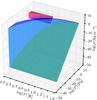 |
Fig. 1 H2 (blue) and He (red) phase diagrams. For clarity, only a part of the upper, almost constant density condensed phases of both species and the low-density gas phase of He are shown. |
2. Gravitational stability of a fluid mixture
In a fluid consisting of K different components i, the total mixture number density is n = ∑ ini, the mixture mass density is ρ = ∑ iρi with ρi = mini, and the mixture pressure is P = ∑ iPi. In the case of an ideal gas, Dalton’s law states P = ∑ ixiPi. Each component has a molecular fraction xi = ni/n and a mass fraction wi = mi/m with m = ∑ iximi.
The notion of global temperature in a system with long-range forces is an unsettled topic as the key assumption of extensivity in thermodynamics breaks down in long-range force systems (e.g. Padmanabhan 1990). When dealing with particle systems we can however always define the temperature as proportional to the residual kinetic energy when the bulk translational, expansional, and rotational velocities are subtracted, be it globally or locally. Strictly, this definition is operational and useful only if the velocity distribution is unimodal and its second order moment exists. Further detailed discussion about this topic would be out of scope, as in this article we consider either global or local temperatures for particle systems with no or negligible amount of ordered motion, so the stated temperature is equivalent to the particle kinetic energy. The high degree of collisionality in molecular interactions ensures the rapid destruction of any initial correlations leading to the convergence towards thermal states.
2.1. Jeans instability
Considering a fluid mixture as a one-component fluid using average quantities such as the density ρ and pressure P, the Jeans instability criterion (see Appendix A.1) would be 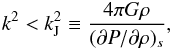 (1)where k is the wavenumber, kJ the critical Jeans wavenumber, and G the gravitational constant. This is, however, inappropriate if each component has a different mean square velocity, which is the case for an isothermal fluid with different molecular masses.
In order to correctly predict the stability of a many-component fluid mixture with different densities ρi and partial pressure Pi, each component has to be treated individually: the Grishchuk-Zeldovich criterion (see Appendix A.2), which is the sum of each component Jeans’ criteria, reads 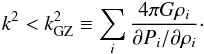 (2)
(2)
2.1.1. Ideal gas mixture
A fluid far from the condensed phase can be approximated with the ideal gas law 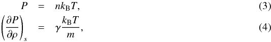 where kB is the Boltzmann constant, γ the adiabatic index, and m the molecular mass. The partial pressures can be calculated using Dalton’s law. Equation (2) becomes
 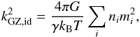 (5)where id stands for ideal gas. This equation differs from Eq. (1), which in the ideal gas case becomes
 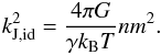 (6)In the case where all components have the same temperature kGZ,id ≥ kJ,id independent of the molecular fractions xi = ni/n and molecular mass mi. In the case of a H2-He mixture, the maximum
  at xH2 = 0.67.
2.1.2. van der Waals fluid mixture
When approaching a phase transition, the ideal gas law does not take into account condensations and does not yield correct values anymore. We showed in FP2015 that the van der Waals equation of state (van der Waals 1910) describes a phase transition rather well provided that the Maxwell construct is taken into account (Clerk-Maxwell 1875; Johnston 2014), i.e. 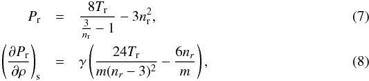 in gaseous and solid/liquid form with the reduced values Pr = P/Pc, Tr = T/Tc, nr = n/nc and the critical pressure, temperature and density Pc, Tc and nc. In the case of a phase transition, Pr = const (Maxwell construct) and (∂Pr/∂ρ)s = 0.
The Maxwell line is very similar to the laboratory condensation line for H2 in a T−P diagram as can be seen in Fig. 2, but is rather off for He, especially at low temperatures. As in the astrophysical context, correctly representing the H2 phase transition is essential for our study. A H2 phase transition always occurs at a lower pressure-temperature ratio than for He.
In the phase transition regime (∂P/∂ρ)s = 0, varying density allows the pressure to remain constant. This is a crucial property for this work, since gravitational contraction is no longer compensated by pressure increase. We show in Appendix A.2 that a two-component fluid is always gravitationally unstable as soon as (∂Pi/∂ρi)s = 0 for any component i. In a similar fashion, the same can be deduced for n-component fluids (Grishchuk & Zeldovich 1981).
2.2. Plane-parallel collapse
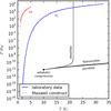 |
Fig. 2 H2 and He laboratory data and van der Waals vapour curve derived from Maxwell construct. Adiabatic compression curves of an initial sphere to sheet-, filament- and point-like geometries for interstellar conditions (T = 10 K, P = 10-12 Pa) are shown, as explained in Appendix B. Sheet-like collapses are allowed to reach the phase transition regime even without cooling. Cooling would displaces the curves to lower temperature. |
Lin et al. (1965) and Zel’dovich (1970) show that a plane-parallel collapse, leading to a sheet-like geometry, is a faster collapse than filament- or point-like geometries. This has been confirmed using numerical simulations by Shandarin et al. (1995).
In addition, as shown in Appendix B.1, the adiabatic matter compression of a sheet-like geometry leads to a finite increase of potential energy, leading to a maximum relative temperature increase of only 2.1, while the energy diverges logarithmically in a filament-like geometry and as Z1/3 in a point-like geometry, where Z = ρfinal/ρinitial is the density compression. This can be seen in Fig. 2 which shows how a sphere moves in this diagram when adiabatically compressed towards a sheet, filament, or point initially in interstellar conditions (T = 10 K, P = 10-12 Pa). Whereas the temperature is quickly increasing with filament- and point-like geometries, in the sheet-like geometry it only rises to ~ 21 K, which is well below the 33 K critical temperature of H2.
When taking radiative cooling into account, the temperature increase by contraction is even smaller. In Appendix B.2 we show that the opacity of a sheet-like collapse is barely increasing. If the initial medium is transparent, the final sheet is also transparent. On the other hand, in filament- and point-like collapses the opacity increases approximately as a power 1/2 or 2/3 of compression, quickly reaching a full opacity regime able to stop the collapse.
2.3. Lennard-Jones mixtures
The Jeans instability of Eq. (2) requires thermal equilibrium and is simplified by only considering linear perturbations. It does not predict its non-linear evolution when unstable. This is a motive to use molecular dynamical simulations with a Lennard-Jones potential in addition to gravity for studying such non-linear phenomena.
The Lennard-Jones potential ![\begin{eqnarray} \Phi_{\name{LJ}}(r) = 4\frac{\epsilon}{m}\left[\left(\sigma \over r\right)^{12} - \left(\sigma \over r\right)^{6}\right] \end{eqnarray}](/articles/aa/full_html/2016/07/aa26975-15/aa26975-15-eq66.png) (9)reproduces the van der Waals equation of state when in equilibrium conditions using the following relations (Caillol 1998):
(9)reproduces the van der Waals equation of state when in equilibrium conditions using the following relations (Caillol 1998): 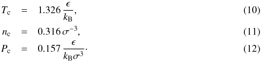 For a fluid mixture, we use the usual Lorentz-Berthelot combining rule for the Lennard-Jones potential between two molecules
 ![\begin{eqnarray} \Phi_{\name{LJ}}(r_{ij}) = 4\frac{\epsilon_{ij}}{m_i}\left[\left(\sigma_{ij} \over r_{ij}\right)^{12} - \left(\sigma_{ij} \over r_{ij}\right)^{6}\right] \label{equ:phiij} , \end{eqnarray}](/articles/aa/full_html/2016/07/aa26975-15/aa26975-15-eq68.png) (13)where
(13)where  and
and  (Lorentz 1881; Berthelot 1898). The most accurate mixing rules for energy and distance are (Banaszak et al. 1995; Chen et al. 2001)
 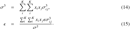 Since Tc ∝ ϵ and nc ∝ σ-3, we have nc/nc,α = (σ/σα)-3 and Tc/Tc,α = ϵ/ϵα. Using Eq. (7), we find Pc = (8/3)Tcnc, and therefore Pc/Pc,α = (σ/σα)-3·(ϵ/ϵα).
As in the ideal gas case, using these mixing properties to calculate kJ in analogy to Eq. (1) instead of using Eq. (2) would lead to different results. In the ideal gas case, the biggest difference is ~ 10%, but in the present case of a van der Waals fluid the difference can be much bigger, for example kJ always returns a finite number if the critical temperature of the mixture Tc> 1, whereas kGZ can nevertheless be infinite if one of the components is in a phase transition.
2.3.1. Binary mixture
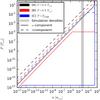 |
Fig. 3 van der Waals phase diagram with Maxwell construct for the H2 – He mixture, each species considered as independent. |
Simulation parameters.
Considering a fluid consisting of two components α and β, we define 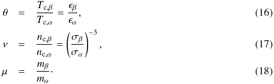 The following Lennard-Jones properties can be derived using Eqs. (13)–(18):
  and the following van der Waals mixture properties:
 ![\begin{eqnarray} {n_\name{c,x} \over n_\name{c,\alpha}} &=& \left[x_\alpha^2 + {x_\alpha x_\beta\over 4}\left(1 + \nu^{-1/3} \right)^3 + {x_\beta^2 \over \nu}\right]^{-1} \ ,\\ {T_\name{c, x}\over T_\name{c, \alpha}} &=& {n_\name{c,x} \over n_\name{c,\alpha}}\left[x_\alpha^2 \,\nu^{1/3} + {x_\alpha x_\beta\,\theta^{1/2} \over 4}\left(1 + \nu^{-1/3} \right)^3 + {x_\beta^2\theta \over \nu} \right] ,\\ \label{equ:px} {P_\name{c,x} \over P_\name{c, \alpha}} &=& {n_\name{c,x} \over n_\name{c,\alpha}}\cdot {T_\name{c, x}\over T_\name{c, \alpha}} , \end{eqnarray}](/articles/aa/full_html/2016/07/aa26975-15/aa26975-15-eq213.png) where xβ = 1−xα. Without loss of generality we choose θ< 1.
where xβ = 1−xα. Without loss of generality we choose θ< 1.
Three different cases can be distinguished, as shown in Fig. 3:
-
1.
Tc,β<Tc,α<T Having the temperature above both critical values, neither component can be in a phase transition and kGZ is always finite.
-
2.
Tc,β<T<Tc,αβ is still above the critical temperature and cannot be in a phase transition, but α may or may not be in a phase transition depending on nα.
-
3.
T<Tc,β<Tc,α Having the temperature below both critical temperatures, both components can be in a phase transition. At equal component number density, α is faster in a phase transition, but theoretically, at low nβ, β could be in a phase transition without α, but this hardly ever happens in reality.
These three cases are studied using computer simulations (see Table 1).
2.3.2. Hydrogen-helium mixture
The critical temperature of H2 and He are 32.97 and 5.19 K, whereas their usual Lennard-Jones ϵ values are 36.4 and 10.57 kBK. This is in conflict with the temperature conversion of Eq. (16), as θH2−He = 6.35 using critical temperatures whereas θH2−He = 3.44 using the Lennard-Jones ϵ values. The same is the case to a lesser degree for the critical density.
All performed simulations are molecule independent, but θ, ν, and μ need to be defined. These values were set using Tc, nc, and the molecular mass of laboratory He and H2 data (Air Liquide 1976). The goal of this article is to understand the role of a secondary component in a fluid presenting a phase transition together with gravity. In molecular clouds, the most likely case of a phase transition is Tc,H2>T>Tc,He, thus it is important to have a correct (Tc,He/Tc,H2) fraction.
2.3.3. Virial theorem
In FP2015, the Lennard-Jones potential has been decomposed in attractive and repulsive terms: ΦLJ = Φa + Φr. In a binary mixture, we have to further distinguish the one-component terms Φα2 and Φβ2, and the cross-terms Φαβ and Φβα (see Eq. (13)).
In analogy with Eq. (5) of FP2015, the virial theorem becomes as follows:  (24)There are two negative, attractive terms, and two positive, repulsive terms. If the attractive and repulsive terms equalize each other, the system is in virial equilibrium.
In the case of a homogeneous density and species distribution of mass M, the energy terms are 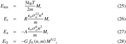 with fG> 0 depending on the geometry. The repulsive and attractive constants are
 ![\begin{eqnarray} R &=& c_\name{r} \left[x^5_\alpha + \theta\,\nu^{-4}x^5_\beta + {\theta^{1/2} \over 2^{12}}\left(1 + \nu^{-1/3}\right)^{12}\left(x_\alpha x_\beta^4 + x_\alpha^4 x_\beta\right)\right], \\ A &=& c_\name{a} \left[x^3_\alpha + \theta\,\nu^{-2}x^3_\beta + {\theta^{1/2}\over 2^{6}}\left(1 + \nu^{-1/3}\right)^{6}~\left(x_\alpha x_\beta^2 + x_\alpha^2 x_\beta\right)\right], \end{eqnarray}](/articles/aa/full_html/2016/07/aa26975-15/aa26975-15-eq242.png) where the lattice coefficients cr and ca depend on the specific crystal lattice (FP2015), which are of importance for the solid phase. Figure 4 shows R and A as functions of an abundance number fraction.
where the lattice coefficients cr and ca depend on the specific crystal lattice (FP2015), which are of importance for the solid phase. Figure 4 shows R and A as functions of an abundance number fraction.
 |
Fig. 4 R/cr and A/cavalues as a function of xα for a H2-He mixture. |
The above terms are for a fluid with no spatial separation of the species, i.e. a fluid in its initial state. The terms predict how an unstable fluid evolves. However, once a phase transition or a gravitational collapse happens, the species may separate. In that case, the terms have to be calculated for each species independently, using xα = 1 and 0, respectively.
2.3.4. Unvirializable densities
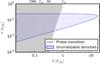 |
Fig. 5 van der Waals phase transition and unvirializable density for a binary mixture with xα = 0.75. |
The sum of the Lennard-Jones and kinetic terms must be positive as the gravitational term is negative: EG< 0 <Er + Ea + Ekin. This is the case if  (31)There can be no virial equilibrium for any mass M> 0, if the attractive Lennard-Jones term dominates the kinetic and repulsive terms. We define the unvirializable density domain as follows:
 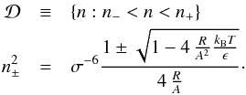 (32)If the term in the square root is negative, there is no real solution and therefore no unvirializable densities. This is the case if
 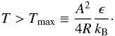 (33)Figure 5 shows the n± values and the domain of the van der Waals phase transition for H2-He mixtures with a molecular fraction of xα = 0.75. There are unvirializable densities above the critical temperature Tc up to Tmax even though no phase transition is possible.
The domain of phase transition does not change a lot for the different xH2> 0, as the H2 phase transition temperature remains the same and the density changes as nx = x·n. It is at much lower temperatures for xH2 = 0, as there is no H2 anymore and the phase transition domain switches to He.
The evolution of fluids with unvirializable densities depends whether they are in a phase transition or not. If these fluids are in a phase transition, there is a gravitational instability independent of M (see Sect. 2.1.2), which leads to a collapse and the formation of bodies of small mass. If they are not in a phase transition, there is only a gravitational collapse above a certain mass M (see Eq. (2)). Below that mass, clumps form, which leads to an augmentation of the kinetic and repulsive Lennard-Jones terms until Eq. (31) is fulfilled, at which point an equilibrium is reached and the fluid may remain stable.
2.3.5. Dynamical friction
When discussing gravitational collapses, the concept of dynamical friction (Chandrasekhar 1943) is important, since heavy objects may condensate from the gas and start to precipitate, i.e. move with respect to the gas in the local gravity field. Considering a uniform density and Maxwellian velocity distribution, the dynamical friction of a heavy object of mass mh reads ![\begin{eqnarray} {\dd \vec{v}_\name{h} \over \dd t} = -{4\pi G^2 m_\name{h}\,\rho \log(\Lambda) \over v_\name{h}^3} \left[\name{erf}(X)-{2X \over \sqrt{\pi}}\exp\left(-X^2\right)\right]\vec{v}_\name{h} , \end{eqnarray}](/articles/aa/full_html/2016/07/aa26975-15/aa26975-15-eq264.png) (34)where log (Λ) is the Coulomb logarithm and
(34)where log (Λ) is the Coulomb logarithm and  . For the qualitative analysis needed in this work, it is enough to state
 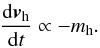 (35)This can be used in different cases. First, He is twice as heavy as H2 and can therefore be considered a heavy object and in some conditions lead to sediment faster than H2. Secondly, when H2 is in a phase transition, H2 ice grains may sediment faster than He.
3. Method
For all of the simulations, the Large-Scale Atomic/Molecular Massively Parallel Simulator (LAMMPS) is used (Plimpton 1995). The use of its short-range Lennard-Jones solver and long-range gravitational solver, super-molecules, and the rRESPA time integrator are discussed in FP2015.
We recall the following super-molecule properties, where η is the number of molecules per super-molecule, 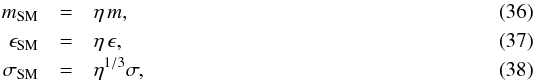 where m, σ, and ϵ are the values for one molecule. The gravitational constant, described in molecular dynamics units (σ = ϵ = m = 1), is
 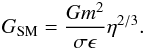 (39)In order for the gravitational force between two super-molecules to be consistently small compared to the intermolecular forces, η should satisfy the following constraint:
 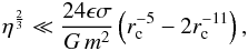 (40)where rc is the cut-off radius in σ units (set to rc = 4 in the simulations).
Two molecules are considered as bound in LAMMPS if their distance is smaller than 1.3625σ. A clump of bound molecules can be either gaseous or condensed, dependent whether its temperature is above or below the critical value.
Initially, the fluid is uniformly distributed in a periodic cubic box. To reproduce the most generic plane-parallel collapse first, as explained in Sect. 2.2, a velocity perturbation in form of a small plane sinusoidal wave in the x direction is superposed to the fluid’s Maxwellian velocity distribution. The perturbation strength is of 1%; see FP2015 for how the perturbation is calculated.
3.1. Units
All simulations are performed in dimensionless units and only the ratios of physical quantities matter. The initial properties of a fluid are the ratios of its temperature to the critical value Tc, its number density to the critical value nc, the Lennard-Jones constant ratios θ, ν, the mass ratio μ, the molecular fraction xα and the gravitational potential strength γG. The needed molecule parameters were set in accordance to laboratory H2 and He values 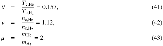 The time unit is defined as the particle crossing time for the box of length L, i.e.
  (44)where V2 = 3NkBT/ ∑ imi, i = 1...N.
The gravitational constant strength is measured by a factor γJ relative to the ideal gas Jeans limit strength GJ, defined as 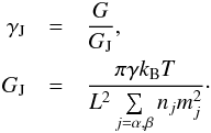 (45)
(45)
3.2. Visualization
In order to visualize the particle snapshots, two-dimensional number density maps are used. The introduced perturbation is along the x-axis, thus the sheet-like collapse is parallel to the yz-plane. For that reason, the density map shows the y- and z-axes where most of the relevant events can be observed. When showing all N particles, smaller aggregates are washed out and barely visible, which is why only a slice of the whole simulation box is shown. Figure 6 shows how this slice is selected: The highest number density is determined in the x direction in order to be centred around the collapse region. From there, the slice width Δx is calculated in order to contain Nslice = fsliceN particles. In that way, the slice width Δx differs for every snapshot, but always contains the same number Nslice of particles.
The number density n and number fraction xα are represented by brightness and colour. As at low density the brightness is maximum and the colour is simply white, the colour map is best visualized in polar coordinates, where n is the radius and xα the angle. Figure 7 shows the colour map used, for better contrasts, the brightness is represented in logarithmic scale.
4. Simulations
In FP2015, we simulated fluids with only one component. We introduced the terms comets for clumps that are principally bound by the Lennard-Jones potential and planetoids for clumps that are principally bound by gravity. If a fluid is in a phase transition, it is important to distinguish between a strong gravitational potential above the ideal gas Jeans criterion and a weak gravitational potential below it. In the strong gravity case, a gravitational collapse happens, leading to the formation of a hot, gaseous planetoid. Phase transitions only happen at the beginning as the fluid heats up above the critical temperature where no solid comets can form.
In the weak gravity case, no gravitational collapse happens and solid comets form thanks to the phase transition. The comets attract each other gravitationally, which leads to the formation of a solid planetoid. During the comet aggregation, the number of bound molecules does not rise. This means that the planetoid only captures comets and no single molecules. Therefore, the fraction of bound molecules is identical to the number of molecules that underwent phase transition.
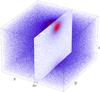 |
Fig. 6 Two-dimensional density map of three-dimensional space. |
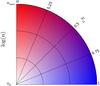 |
Fig. 7 Colour mapping of density map. |
In this article, we compare fluids with different molecular fractions by keeping the physical properties alike (constant T/Tc,α and n/nc,α). By decreasing xα the mean mass per molecule m increases, since mα<mβ. It is therefore not possible to have the same number of molecules per super-molecule η, the same super-molecule mass MSM = mη, and the same gravity GJ ∝ m2η2/3 at the same time.
Since we want to study the reaction of fluids with different xα above and below the ideal gas Jeans criterion, we need to ensure that γJ is >1 or <1 in the compared simulations. For that reason, neither the total mass nor the number of molecules remains the same when comparing fluids with different xα, while γJ remains the same. Since  (Eq. (45)) and η2/3 ∝ m-2G (Eq. (39)), then
  and thus
  . Therefore, changing m by a factor 2 leads to a total mass factor decrease of 32.
Different cases are studied: T = 1.5Tc,α, T = 1.5Tc,β and T = (TCMB/Tc,H2) Tc,α with n = 10-2nc,α and xα = 1, 0.75, 0.5, 0.25, and 0. These initial parameters are shown in Fig. 3. In addition, different densities are used for simulations B75 and C75 to compare cases with n>n− with n<n− (see Sect. 2.3.3). We also study solar system abundances for different total masses and number densities. The simulations are summarized in Table 1.
The simulations with γJ< 1 were run until a steady-state solution was reached. Most simulations with γJ> 1 were stopped once a planetoid formed, which typically happens after ~ 5τ. Even if the resulting fluid did not reached a steady state then, no further developments are expected, as checked in FP2015. A few simulations were run for 15τ to confirm this. At t = 5τ, the planetoid of B75 with γ = 1.5 is 15% hotter than average, whereas unbound molecules are 5% colder. After another 10τ, however, at t = 15τ, the temperature differences are below 1%. Similarly, at t = 5τ, there are very strong regional temperature differences of ≥10% considering subdomains of 1% volume. At t = 15τ, they are ≤5%.
4.1. Above critical temperatures
In this Section, we consider fluids where both Tα and Tβ are above the critical temperature. The number densities corresponding to the different abundance number fractions can be seen in Fig. 3.
4.1.1. Time evolution
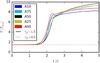 |
Fig. 8 Global temperature as a function of time of the A simulations with γJ = 1.5 and 0.5. |
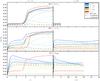 |
Fig. 9 Evolution of the number of bound molecules as a function of time of the A), B), and C) simulations with γJ = 1.5 and 0.5. The simulations with γJ = 0.5 are stopped after 5τ, 30τ, and 20τ for the A), B), and C) simulations, respectively, when no further significant development is expected. |
Figure 8 shows the global temperature evolution of the A simulations (see Table 1). In all simulations, the weakly self-gravitating fluids with γJ = 0.5 and the fluids without gravity are very similar and do not react significantly to the velocity perturbation. On the other hand, as expected for the sufficiently self-gravitating fluids with γJ = 1.5 the introduced perturbation rises exponentially. The reaction time is similar for all number fractions, but the mixtures reach slightly higher temperatures. Keeping in mind that all simulations have the same γJ value, but the total mass differs with M1/M2 = (m1/m2)-5.
To get a deeper understanding of the internal processes, we need to distinguish between the α and β component. Figure 9A shows the fraction of bound molecules in the simulations as a function of time. No phase transition happens above the critical temperature, therefore no comets form in the simulations with γJ = 0 and 0.5. With γJ = 1.5, the gravitational collapse leads to the formation of a planetoid. In its centre, the gravitational pull is strong enough to keep the molecules bound even though the temperature is well above the critical value.
The β-molecules, as they are twice as heavy as the α-molecules, fall faster into the forming planetoid. Indeed, even in A75, with only xβ = 0.25, the fraction of bound β-molecules surpasses the fraction of bound α-molecules for τ> 2.
4.1.2. Planetoid formation
Figure C.1a shows a time sequence of snapshots and super-molecule, comet-size distributions condensed as grains or comets. The parameter Ncomet is the number of super-molecules in one comet and  is the comet size distribution function. At the beginning with t< 3τ, small comets of either α- or β-molecules form. At t = 3τ, a planetoid with N ≈ 0.1Ntot forms consisting of both components. One can already see a dominance of β-molecules, especially in the centre.
Beginning at t = 3τ, and even more clearly at t = 4τ, one can observe the formation of a big core consisting only of β-molecules (isolated β-dot). In the snapshots this corresponds to the planetoid shown as a β-core surrounded by α-molecules. Once the planetoid has reached this form, it reaches a steady state. Its temperature matches the gas temperature, and the temperature fluctuations level out (see FP2015 for more details on planetoid and comet temperatures).
Figure 10 (top) shows the planetoid density of simulation A75 as a function of radius. Even though the fluid consists of only 25%β-molecules, the planetoid consists mostly of β-molecules with fβ = 0.86. The α-molecules are only a small fraction and mostly present in the outer part. The gaseous nature of this body is visible as the density regularly decreases in radii.
4.1.3. Scaling
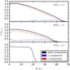 |
Fig. 10 Density of planetoid as a function of the radius of the simulations A75 and B75 with γJ = 1.5 at t = 5τ and B75 with γJ = 0.5 at t = 30τ. |
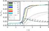 |
Fig. 11 Fraction of bound molecules as a function of time for the simulations A75S with γJ = 1.5 and different Ntot. |
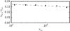 |
Fig. 12 Fraction of bound β-molecules as a function of Ntot for the simulations A75S. |
The scaling of simulations using super-molecules has already been discussed in FP2015. In order to obtain the correct behaviour, the gravitational forces FG need to be small on intermolecular scales compared to the Lennard-Jones forces FLJ, i.e. FG(rc) <FLJ(rc), where rc is the cut-off radius (see Eq. (40)). A turning point can be identified up to which  follows the power-law
  with negative index ξc< −1, whereas after the turning point follows a second power law with index ξp = 1 (see Fig. C.1a). The appearance time of this turning point is independent of Ntot, whereas the size of the comet at the turning point scales as
  , thus Ncomet ≈ 10. This corresponds roughly to the smallest number of nearest neighbours in the condensed phase in 3D for which surface effects start to be dominated by volume effects.
Figure 11 shows the fraction of bound molecules as a function of time for all A75S simulations with Ntot = 503 to 1603. As shown in FP2015, the slight time delay between the simulations can be attributed to the random seed. In any case, the asymptotic final value is physically more important, and is the same for all Ntot when considering both components. The final value of the β-molecules, on the other hand, very slightly declines with increasing Ntot as can be seen in Fig. 12. It follows the power-law  over the range Ntot = 105−106.5.
4.1.4. Extrapolation to physical scale
The simulations should actually represent a H2-He fluid mixture with ~ 1050 molecules. As outrageous as this extrapolation might appear, this is exactly what usually takes place in many other types of simulations (cosmological, galactic, or stellar simulations) because as long as the physical scale invariant aspect of the physics between the macro- and micro-scales are separated by enough orders of magnitude the exact range of scale difference does not matter over dynamical timescales. For longer simulation timescales one can check how the results scale with N by running simulations with different N, which is the reason why we always run the simulations with several N. Extrapolating the previous power law to physical scales, we find that ~ 3% of β-molecules settle inside the planetoid, instead of ~ 15%. Thus the simulations overestimate species segregation, which is to be expected in view of the increased fluctuations when the number of particles decreases. Segregation effects should be treated with caution, as we are extrapolating values in a range that is less than two orders of magnitude or 45 orders of magnitude away. Larger simulations should allow us to better constrain the effective species segregation in realistic conditions.
4.2. Between critical temperatures
In this section, we consider fluids with Tα<Tc,α and Tβ>Tc,β with different component fraction xα. The number density n has been chosen in such a way that for the molecular fractions xα> 0, the α-component with number density nα = xα·n is in a phase transition.
As the temperature of the B simulations is an order of magnitude smaller than in the A simulations, the same is the case for the gravitational potential (see Eq. (45)). For that reason, it is sufficient to use Ntot = 803 for these simulations.
4.2.1. Above the ideal gas Jeans criterion
Figure 9B on the left side shows the time evolution of the fraction of bound molecules for the B simulations with γJ = 1.5. One can see the similarity to Fig. 9A, but the fluids with a high xα value are rising to higher values even before the perturbation is becoming dominant. This is because the α-portion of the fluid is in a phase transition and small ice grains are forming even without the help of gravity. The formed planetoid is gaseous, as can be seen in Fig. 10 (middle). This shows that the phase transition does not have an important effect if γJ> 1 and that the instability can be predicted by the ideal gas Jeans criterion.
The density at the core of the planetoid of simulation B75 is lower than that of A75. This is explained by the fact that by keeping γJ = 1.5, the value for GJ is lower for the B simulations than for the A simulations as GJ ∝ T (see Eq. (45)). Having a lower gravitational potential, the density at which the repulsive Lennard-Jones term and the attractive gravitational term are equal is lower.
The planetoid is still dominated by β-molecules, but there are more α-molecules than in the A75 simulation with fα = 0.26 and fβ = 0.74. As in the A simulations, the core consists of gaseous He, as is clearly visible in Fig. C.1b.
4.2.2. Below the ideal gas Jeans criterion
As can be seen in Fig. 3, the α-component of the simulations B10, B75, B50, and B25 all lie on the Maxwell line and are thus in a phase transition, which implies, according to Eq. (2), that they are gravitationally unstable even with γJ< 1.
The right side of Fig. 9B shows the evolution of the fraction of bound molecules of the B simulations with γJ = 0.5. The timescale is much larger (30τ instead of 5τ in the case of γJ = 1.5), having a smaller gravitational potential, the long-range gravitational term is lower, and therefore the creation of any potential comet or planetoid takes more time.
The one-component fluids, consisting of either uniquely α-molecules (B10) or β-molecules (B00) have already been studied in detail in FP2015. The α-fluid B10 is unstable as it is in a phase transition, whereas the β-fluid B00 is stable as its temperature is above the critical value and no phase transition is possible.
The simulations of fluid mixtures B25, B50, B75 with γJ = 0.5 are all unstable, even gravitationally. We can distinguish a clear difference in the simulations with γJ = 1.5 in that only the α-molecules form comets, whereas the β-molecules remain in gaseous form. Even in the simulation B25, which has only 25% α-molecules, the comets and planetoid consist almost exclusively of α-molecules. This difference between γJ = 1.5 and 0.5 can also be seen when comparing Fig. C.2a with Fig. C.1b.
Figure 10 (bottom) shows the radius of the planetoid at t = 30τ of B75 with γJ = 0.5. Comparing with the planetoid of B75 with γJ = 1.5, we see that the high-gravity planetoid consists mostly of β-molecules in gas phase, whereas the low-gravity planetoid consists of mostly α-molecules in solid phase, surrounded by an atmosphere. Very few β-molecules have been trapped during the planetoid formation, providing an interesting example of a body forming with a distinct composition from the original medium as a result of the initial phase transition state.
4.2.3. Different γJ values
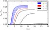 |
Fig. 13 Fraction of bound β-molecules as a function of time for the simulations B75γ. The simulations are stopped once they reach asymptotic values. |
The previous sections show that a fluid in a phase transition above the ideal gas Jeans criterion, i.e. with γJ = 1.5, forms a gaseous planetoid consisting mostly of β-molecules due to a classical ideal gas Jeans collapse. On the other hand, a fluid in a phase transition with γJ = 0.5 forms small α-comets due to the phase transition. These comets are attracted to each other by gravity, leading to the formation of a rocky planetoid, consisting almost exclusively of α-molecules. In this section, we vary γJ from 0.5 to 1.5.
Figure 13 shows the fraction of bound β-molecules. It is rising steeply for fluids with γJ> 1 in accordance with the ideal gas Jeans criterion and the formed planetoid is gaseous and consists mostly of β-molecules. The fluid with γJ = 1 also produces a gaseous planetoid, but the percentage of β-molecules is already dropping a little. Interestingly, in the fluids with 0.7 ≤ γJ< 1, the β fraction is also rising. The instability criterion of Eq. (2) is for all components, not only one of them.
Figure C.2b shows snapshots and comet-size distributions of simulation B75γ with γJ = 0.8. One sees that at first (t ≤ 8τ) only the α-molecules are collapsing and forming a rocky planetoid. Then, owing to the great attractive force of the α-planetoid, many β-molecules gather around it, forming an atmosphere (t = 12τ). A β-atmosphere can also be observed, in a less striking way, for the simulation with γJ = 0.5 in Fig. C.2a. What happens afterwards is very interesting: at t = 16τ, one sees that the rocky planetoid swaps the α- and β-molecules and the heavier β-molecules replace the α-molecules near the centre.
4.3. Below critical temperatures
In this section, to complete the study of binary fluid mixtures, we consider fluids where both Tα and Tβ are below the critical temperature. The number density n has been chosen in such a way that for the molecular fractions xα> 0, the α-component with number density nα = xα·n is in a phase transition.
4.3.1. Above the ideal gas Jeans criterion
The left side of Fig. 9C shows the time evolution of bound molecules of the C simulations with γJ = 1.5. There is a distinct difference compared to the A and B simulations, which form β-planetoids; only the percentage of bound α-molecules rises and the forming planetoid only consists of α-molecules (see Fig. C.3). This is slightly counter-intuitive at first, as one could expect the β-molecules to be even more eager to fall into the planetoid than in the A and B simulations, since the temperature is lower.
Owing to the very low temperature of the C-simulation, however, the α-molecules quickly form comets from the very beginning. These comets are heavier than the β-molecules and decelerate faster into the planetoid.
4.3.2. Below the ideal Gas Jeans criterion
The evolution of the simulations below the ideal gas Jeans criterion is analogous to the B simulations. The fraction of bound α-molecules in the pure α-fluid and the mixture rise, and the fraction of bound molecules of the pure β-fluid remains very low. This is in accordance with Fig. 3 where the α-molecules are unstable but the β-molecules are stable. The simulations C10, C75, C50, and C25 form a rocky α-planetoid, as already seen in the B simulations (see Fig. C.2a).
4.4. Virial theorem
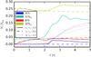 |
Fig. 14 Fraction of bound molecules with cluster mass mcl>mHe as a function of time of simulations in and out of the unvirializable density domain. |
When comparing the simulations above the ideal gas Jeans instability, there is a clear difference between the A and B simulations on one side, and the C simulations on the other. A gaseous β-planetoid forms in the first two, whereas a rocky α-planetoid forms in the latter. Looking at the virial terms of the fluids (see Sect. 2.3.3), Eq. (31) is fulfilled in the A and B simulations, whereas for the C simulation, the density is in the unvirializable domain  . In this Section, we vary the densities of the A and B simulations in order to be in and out of the unvirializable domain.
Figure 14 shows the time evolution of clusters that have a higher mass than one β-molecule (Ncl,α> 2) for the simulations in the unvirializable domain (A7501 and B7501) and below (A75 and B75). A very quick rise of H2 comets for the unvirializable fluid happens, both with and without gravity, which is in accordance with Eq. (31), as neither the repulsive Lennard-Jones term nor the kinetic energy can withhold the attractive Lennard-Jones term thus leading to the formation of comets. Even in simulation A7501, with a temperature above the critical temperature, this comet formation is taking place, even though a phase transition is officially not possible. A slow comet formation only takes place for the virializable fluids.
Once the exponential growth of the perturbation becomes important (t ≥ 2τ), the unvirializable fluids have created an important number of comets heavier than the β-molecules, which fall faster in the forming planetoid as a result of dynamical friction. This can be seen in Fig. 15 where the planetoids of the simulations A75 and B75 consist mostly of β-molecules, whereas the planetoid of B7501 consists mostly of α-molecules. A somewhat special case is A7501, where the planetoids composition is almost perfectly fifty-fifty. This can be explained by the fact that because is is above the critical temperature, the comets are not really solid, but consist of a dense gas that is able to mix easily with β-molecules. Thus, once a α-planetoid has formed using all the heavy α-comets, the β-comets fall into the planetoid and mix with it.
4.5. Influence of β-molecules on α-molecules below the ideal gas Jeans criterion
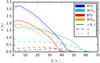 |
Fig. 15 Density of planetoid at t = 5τ as a function of the radius of the simulations in and out of the unvirializable density domain. |
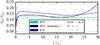 |
Fig. 16 Fraction of bound molecules as a function of time of the simulations B75, B75 with removed β-molecules and B10. γJ = 0.5. |
As can be seen in Fig. 9C, almost no β-molecules form comets if γJ = 0.5 and the percentage of β-molecules in the planetoid is negligible. Granted, the concentration of He around the planetoid rises slightly as can be barely seen in Fig. C.2a. Thus the question can be raised whether a small fraction of a secondary molecule (such as He in the case of molecular clouds) needs to be included in low-gravity simulations. To answer that question, simulation B75 with γJ = 0.5 was run again, but all β-molecules were removed and their mass was equally distributed to the α-molecules to maintain the same gravitational potential.
Figures 16 shows the time evolution of the fraction of bound molecules of the simulations B75, B75 without β-molecules and B10 for comparison. Even though the two B75 simulations are similar, there are differences to be observed. The fraction of bound α-molecules of the simulation B75 should correspond to the total fraction of bound molecules of the simulation without β-molecules, but the latter is higher; the β-molecules in B75 have a damping effect on the comet formation. In addition, the simulation without β-molecules is rising to a higher value at the end of the simulation.
The inclusion of a small fraction of a secondary molecule does change the look of the simulation by damping the comet formation of α-molecules. For that reason, the inclusion of secondary molecules in more realistic simulations is useful.
4.6. Physical systems
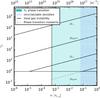 |
Fig. 17 γJ of different total fluid masses at T = 10 K, as a function of number density, indicating either ideal gas Jeans instability, or instability owing to phase transition. |
Up to now, we have looked at theoretical models, varying xα from 0 to 1, and setting the temperature and density as a fraction of the respective α critical values. The critical values for H2 are Tc = 32.97 K and nc = 9.34 × 1027 m-3. In astrophysical conditions, the He mass fraction is between wHe,SS = 0.2741 for the solar system (Lodders 2003) and wHe,MW = 0.2486 for the initial Big Bang mixture (Cyburt et al. 2008), which translates to number fractions xHe,SS = 0.1598 and xHe,MW = 0.1428.
Figure 17 shows γJ as a function of the number density for solar system abundances (x = 0.16) and T = 10 K with total masses equal to the Moon, Earth, Jupiter, and Sun. H2 is then in a phase transition for n> 4 × 1024 m-3; only a Moon mass or below can be in a phase transition and below the Jeans criterion. The fluid is unvirializable for n> 6 × 1026 m-3.
If we go to a lower temperature, say the CMB 2.7 K, a H2 phase transition takes place for n> 1012 m-3. In that case, fluids with Earth mass would be chemically unstable below the ideal gas Jeans criterion for n ≤ 3 × 10²¹ m-3 and with Jupiter mass for n ≤ 3 × 10¹⁶ m-3. Fluids with Sun mass, on the other hand, cross γJ = 1 only in the gaseous phase of H2. The lowest unvirializable density n− = 6 × 1026 m-3 does not change a lot with temperature.
The number of FFT mesh cells NFFT ∝ L3 and the simulation timescale τ ∝ L both directly depend on L ∝ n− 1/3, and the total calculation duration scales as tsim ∝ τ·NFFT ∝ n− 4/3. For that reason, simulating a fluid at CMB temperature with densities below 1020 m-3 would translate to extremely long simulation run times with today’s computers. In addition, the upper limit for the mass of super-molecules is mSM,max ≈ 5 × 10⁻⁶M⊕ (see Eq. (40)). Thus, the minimum number of super-molecules Ntot, min = M/mSM,max is ~ 2 × 10⁵, 6.5 × 10⁷, 6.5 × 10¹⁰ for simulating an Earth, Jupiter, and Sun mass, respectively. For that reason, for the time being we content ourselves to studying systems up to total mass comparable to the Earth mass.
4.6.1. Planetoid formation
Three simulations were run at a temperature of T = 10 K, which is above the critical temperature of He and below that of H2, and thus in a similar regime as the B simulations. Two simulations have a total mass equal to the Moon, with n ≈ 1027 m-3 which is above the ideal gas Jeans criterion and in the unvirializable domain, and n ≈ 1026 m-3, which is below the Jeans criterion, and one has a total mass equal to the Earth and with n ≈ 1024 m-3, which is above the criterion. The simulation parameters are given in Table 1.
Figure 18 shows the snapshot and comet-size distribution of the three simulations after the formation of a planetoid. The fluid of SSE04 is above the ideal gas Jeans criterion and we observe the formation a He-planetoid, surrounded by H2, similar to Sect. 4.2.1. The evolution of simulation SSM02, which is below the ideal gas Jeans criterion, leads to the formation of a rocky H2 planetoid, similar to Sect. 4.2.2.
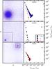 |
Fig. 18 Snapshots and comet-size distributions of the simulations SSM01, SSM02, and SSE04. The slice selects in depth 20% of the super-molecules. The squares in the two lower left frames are the same size as the next upper frame. |
In the case of SSM01, the density lies in the unvirializable domain, resulting in a formation of many H2-grains that are heavier than the He-atoms from the very beginning. This leads to the formation of a H2-planetoid similar to Sect. 4.3.1.
5. Conclusions
In our first article, FP2015, we studied the gravitational instability of a fluid in a phase transition. We extrapolated the results to the ubiquitous H2 and showed that the formation of cold, mostly undetectable comet- and even planet-sized rocky H2 clumps is very possible. The use of only one component gives a good first impression, but in cosmic gases, there is a mass fraction of w ≈ 25 ± 2% He atoms.
In the present work, we studied binary fluid mixtures analytically and via numerical simulations. The results show that, depending on the circumstances, either He or H2 planetoids can form.
5.1. Analytic results
The stability of a multicomponent fluid mixture has already been studied in the literature, mostly to study fluid binaries consisting of baryonic and dark matter. The wave number below which a fluid mixture is unstable is the sum of the Jeans wave-numbers of each component. Since the Jeans wave number is inversely proportional to  , which is equal to zero in the case of a phase transition, a fluid mixture is unstable as soon as one of its components is in a phase transition. Physically what happens is that when one species is in a phase transition, an overdensity only increases its condensed phase fraction at constant pressure, instead of increasing pressure and producing no global force to counter gravity. The transformation from the gas to the condensed phase continues until the species is fully condensed.
We studied the evolution of unstable fluid mixtures with the widely used Lennard-Jones intermolecular potential, which reproduces the H2 phase transition very well (but it reproduces the He transition, which is not essential in this work, less well). We showed, using the virial analysis of Lennard-Jones fluid mixtures, that there is a unvirializable density-domain within which the attractive forces dominate the repulsive forces for any total mass M and no virial equilibrium is possible. These states can be reached in strongly dynamical situations (e.g. during collapses) and are able to produce condensed comets particularly quickly. Dynamical friction is important to separate species and condensed comets. For instance, if H2 is in a phase transition, the formed H2 comets are heavier than the He-molecules, and precipitate in a gravitational field, producing almost pure H2 bodies.
There are three reasons to concentrate on plane-parallel initial collapses, as described in more detail in Appendix B:
-
1.
In typical cosmic conditions, the fastest collapsing geometry issheet-like, not filament- or point-like.
-
2.
The adiabatic matter compression during collapse leads to the least heating in sheet-like geometry: in a sheet-like adiabatic collapse the gravitational energy released to the fluid is finite and amounts to a maximum increase of temperature by only a factor of about two, while in filament-like collapses the temperature diverges logarithmically as a function of filament radius, and in point-like collapses the temperature diverges as the inverse sphere radius.
-
3.
Radiative cooling is the easiest in sheet-like collapse. Indeed the absorption probability in sheet-like geometry remains almost unchanged for any compression, and an initially transparent medium remains transparent, whereas the probability converges to one in filament-like and point-like geometries. Therefore, radiative cooling is barely slowed down in sheet-like collapses and, unlike in spherical or filament collapses, opacity is unable to prevent density from reaching high values. This is a crucial point for this study, as the ISM conditions are commonly thought to be far away from the H2 phase transition conditions.
5.2. Simulations
As in FP2015, we used super-molecules to combine the Lennard-Jones intermolecular potential together with the gravitational potential in numerical simulations. Several binary fluid mixtures were studied using two components: α and β. Their respective properties (the most important being mα/mβ< 1 and Tc,α/Tc,β> 1) were chosen to mimic a H2-He fluid, but the general properties of the fluids were made molecule independent.
Three temperature domains can be defined: (A) above both critical temperatures; (B) between the critical temperatures; and (C) below both critical temperatures. In all three cases, the molecular fraction was varied and the fluids were simulated above and below the Jeans criterion. We used different numbers of molecules to test the scaling of the simulations. The precise number of super-molecules is not important for dynamical processes, but we found a weak dependence for segregation effects in the sense that coarser simulations exaggerate these effects.
In case (A), both components are gaseous and an introduced perturbation does not grow when the gravitational potential is below the Jeans criterion. When above the Jeans criterion, the fluid collapses and forms a gaseous planetoid. The β-molecules are twice as massive as the α-molecules, and fall faster into the planetoid. For that reason, the planetoid consists mostly of β-molecules, surrounded by an α-atmosphere. This is independent of the molecular fraction xα, even at very high xα-values, the planetoids consists mostly of β-molecules.
In case (B) and (C), the number density of the fluids was chosen so that the α-component is in a phase transition for all xα> 0. In fact, both cases are very similar since in both cases the β-component is not in a phase transition. When the fluids are below the Jeans criterion, an instability happens because of the phase transition of the α-component, which leads to the formation of H2 comets and ultimately a rocky α-planetoid. This planetoid is surrounded by a β-atmosphere, which is getting more important with increasing gravitational potential. As in case (A), the molecular fraction xα does not matter, even at very low xα-values, the planetoid still consists almost exclusively of α-molecules.
A suprising observation occurs for cases (B) or (C) above the Jeans criterion. In that case, there is a race between the formation of small α-grains owing to the phase transition and the exponential growth of the perturbation. The heaviest bodies are decelerated faster and fall into the forming planetoid first. When the α-component is either gaseous or only forming very few and small comets, a β-planetoid forms. On the other hand, if the α-component forms many grains that are heavier than the β-molecules, an α-planetoid forms. We showed in the simulations that this race between α and β is linked with the unvirializable density domain . If a fluid reaches this domain, the α-component wins, otherwise the β-component wins.
5.2.1. Solar system abundances
In addition to the above-mentioned simulations, fluids with solar system abundances and Moon or Earth mass were simulated. As shown in Fig. 17, a fluid with Earth mass cannot be below the Jeans criterion and still in a phase transition, but with Moon mass, this is possible. In that case, a rocky H2 planetoid results. With a mass as low as the Moon, the fluid needs to be very dense to be above the Jeans criterion. In fact, the fluid would lie in the unvirializable density-domain and, thereby, a H2-planetoid forms. For a fluid with Earth mass, on the other hand, even a relatively low-density fluid is still above the Jeans criterion. The result is a gaseous He planetoid with a H2 atmosphere.
5.3. Instability in H2-He fluid
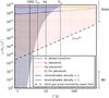 |
Fig. 19 Gravitational instabilities at different temperatures and densities for a fluid with Jupiter mass. |
Figure 19 shows different possible planetoid and comet formations due to gravitational instability for a fluid with Jupiter mass. A fluid is gaseous if it is below the phase transition domain and a fluid is solid or liquid if above. When the density is in the phase transition, it can rise without an increase of pressure.
There can be no formation below the Jeans criterion if the fluid is not in a phase transition. Most of the planetoids due to an ideal gas Jeans collapse consist of gaseous He, but if the fluid is in the unvirializable domain , then a H2 planetoid forms. This H2 planetoid can be solid/liquid or gaseous depending on its temperature. If gaseous, He is able to percolate down, slowly transforming it into a He planetoid.
If the fluid is in a phase transition, we have to distinguish between a collapse above the ideal Jeans criterion, which leads to a gaseous He planetoid except in the unvirializable domain, where it becomes a rocky H2 planetoid, and in a collapse below the ideal Jeans criterion, which also leads to a rocky H2 planetoid.
The usual average density domain of molecular clouds lies between 108 and 1012 H2/ m3 and, with such a density, a H2 phase transition is only possible at temperatures below ~ 5 K. However, molecular clouds are observed to follow a fractal mass distribution over a minimum of 4–6 orders of magnitude in column densities, so the average density is not a quantity to characterize molecular clouds properly. Since we know that stars form with densities ~ 1029 H2/ m3, by continuing this argument, intermediate states covering all this density interval have to exist.
Fluids with a high total mass, especially with stellar mass or above, reach the ideal gas Jeans criterion very quickly leading to gaseous He-planetoids. Fluids with lower total mass, however, as for example the cold globules observed in the Helix nebula, especially with Earth mass and below, have the ideal gas Jeans criterion at much higher densities and are in the phase transition domain before being above the ideal gas Jeans criterion.
5.4. Perspectives
This and the previous FP2015 study show that the cold ISM physics is much richer than previously imagined. The formation of substellar gaseous or rocky condensed bodies by the H2 phase transition combined to gravity, appears natural once we recognize that collapses proceed most of the time along the sequence pancake, filament, and point, and in the first sheet-like phase high densities allowing a H2 phase transition can be reached if the initial medium temperature is below ~ 15 K. This temperature limit would be even higher if radiative cooling had been considered. In the isothermal case this limit is ~ 33 K.
Most of the ISM cold gas must therefore pass over molecular cloud lifetimes (~ 106−108yr) through such brief (~ 102−104yr) singular sheet-like collapses where density diverges but not temperature. Observationally, such events are difficult to detect because of the limited increase of temperature, opacity, and column density all along the collapse, while reaching high volume densities. When seen edge-on such sheet-like collapses would look like filaments.
The simulations we were able to perform are still very limited in total mass. Including He is necessary but this provides a number of complications with respect to the pure H2 case, and widens the general picture found in FP2015. Combining the accumulated experience of large-scale gas phase simulations by other authors (e.g. Renaud et al. 2013; Butler et al. 2015), we can easily extrapolate what larger simulations should produce with micro-AU resolution. Instead of one planetoid per simulation box, pc-sized sheet-like collapses should show filaments with longer lifetimes, which would funnel H2 condensed bodies and produce a spectrum of planetoids, comets, and occasionally stars. The leftover condensed cold substellar bodies should then start to evaporate according to the ambient radiation flux and depth of their gravitational potential. The lifetime of such bodies should be short near the centre of galaxies, but much longer at the periphery of galaxies, or even in intergalactic space, especially in cosmic filaments. One can postulate that, especially at the periphery of disk galaxies where the radiation heating is low, some fraction of the dark baryons can be trapped in the form of such condensed bodies. We plan to pursue further simulation work to deepen our understanding of the processes associating phase transition with gravitational dynamics.
Acknowledgments
This work is supported by the STARFORM Sinergia Project funded by the Swiss National Science Foundation. We thank the LAMMPS team for providing a powerful open source tool to the scientific community.
References
- Air Liquide. 1976, Gas Encyclopedia (Elsevier) [Google Scholar]
- Banaszak, M., Chiew, Y. C., & Radosz, M. 1995, Fluid Phase Equilibria, 111, 161 [CrossRef] [Google Scholar]
- Becker, A., Lorenzen, W., Fortney, J. J., et al. 2014, ApJSS, 215, 21 [NASA ADS] [CrossRef] [Google Scholar]
- Berthelot, D. 1898, Comptes rendus hebdomadaires des séances de l’Académie des Sciences (Paris: Gauthier-Villars) , 126, 1703 [Google Scholar]
- Bolatto, A. D., Wolfire, M., & Leroy, A. K. 2013, ARA&A, 51, 207 [Google Scholar]
- Butler, M. J., Tan, J. C., & Van Loo, S. 2015, ApJ, 805, 1 [NASA ADS] [CrossRef] [Google Scholar]
- Caillol, J. M. 1998, J. Chem. Phys., 109, 4885 [Google Scholar]
- Chandrasekhar, S. 1943, ApJ, 97, 255 [NASA ADS] [CrossRef] [Google Scholar]
- Chen, J., Mi, J.-G., & Chan, K.-Y. 2001, Fluid Phase Equilibria, 178, 87 [CrossRef] [Google Scholar]
- Clerk-Maxwell, J. 1875, Nature, 11, 357 [NASA ADS] [CrossRef] [Google Scholar]
- Cyburt, R. H., Fields, B. D., & Olive, K. A. 2008, J. Cosmol. Astropart. Phys., 11, 012 [Google Scholar]
- de Carvalho, J. P. M., & Macedo, P. G. 1995, A&A, 299, 326 [NASA ADS] [Google Scholar]
- Draine, B. T. 2011, Physics of the Interstellar and Intergalactic Medium (Princeton University Press) [Google Scholar]
- Elmegreen, B. G., & Scalo, J. 2004, ARA&A, 42, 211 [NASA ADS] [CrossRef] [Google Scholar]
- Füglistaler, A., & Pfenniger, D. 2015, A&A, 578, A18 [NASA ADS] [CrossRef] [EDP Sciences] [Google Scholar]
- Grishchuk, L. P., & Zeldovich, Y. B. 1981, Sov. Astron., 25, 267 [NASA ADS] [Google Scholar]
- Jeans, J. H. 1902, Roy. Soc. London Phil. Trans. Ser. A, 199, 1 [Google Scholar]
- Jog, C. J., & Solomon, P. M. 1984a, ApJ, 276, 127 [NASA ADS] [CrossRef] [Google Scholar]
- Jog, C. J., & Solomon, P. M. 1984b, ApJ, 276, 114 [NASA ADS] [CrossRef] [Google Scholar]
- Johnston, D. C. 2014, Advances in Thermodynamics of the van der Waals Fluid (Morgan & Claypool) [Google Scholar]
- Koci, L., Ahuja, R., Belonoshko, A. B., & Johansson, B. 2007, J. Phys. Condensed Matter, 19, 016206 [NASA ADS] [CrossRef] [Google Scholar]
- Landau, L. D., & Lifshitz, E. M. 1975, The classical theory of fields (Pergamon Press) [Google Scholar]
- Lin, C. C., Mestel, L., & Shu, F. H. 1965, ApJ, 142, 1431 [NASA ADS] [CrossRef] [Google Scholar]
- Lodders, K. 2003, ApJ, 591, 1220 [NASA ADS] [CrossRef] [Google Scholar]
- Lorentz, H. A. 1881, Annalen der Physik, 248, 127 [Google Scholar]
- Padmanabhan, T. 1990, Phys. Rep., 188, 285 [NASA ADS] [CrossRef] [MathSciNet] [Google Scholar]
- Pfenniger, D., & Combes, F. 1994, A&A, 285, 94 [NASA ADS] [Google Scholar]
- Pfenniger, D., Combes, F., & Martinet, L. 1994, A&A, 285, 79 [NASA ADS] [Google Scholar]
- Plimpton, S. 1995, J. Comput. Phys., 117, 1 [Google Scholar]
- Renaud, F., Bournaud, F., Emsellem, E., et al. 2013, MNRAS, 436, 1836 [NASA ADS] [CrossRef] [Google Scholar]
- Safa, Y., & Pfenniger, D. 2008, Eur. Phys. J. B, 66, 337 [NASA ADS] [CrossRef] [EDP Sciences] [Google Scholar]
- Saumon, D., Chabrier, G., & van Horn, H. M. 1995, ApJSS, 99, 713 [NASA ADS] [CrossRef] [Google Scholar]
- Shandarin, S. F., Melott, A. L., McDavitt, K., Pauls, J. L., & Tinker, J. 1995, Phys. Rev. Lett., 75, 7 [NASA ADS] [CrossRef] [Google Scholar]
- Streett, W. B. 1973, ApJ, 186, 1107 [NASA ADS] [CrossRef] [Google Scholar]
- van der Waals, J. D. 1910, Koninklijke Nederlandse Akademie van Wetenschappen Proceedings, Series B Physical Sciences, 13, 1253 [Google Scholar]
- Volkov, E., & Ortega, V. G. 2000, MNRAS, 313, 112 [NASA ADS] [CrossRef] [Google Scholar]
- Vorberger, J., Tamblyn, I., Militzer, B., & Bonev, S. A. 2007, Phys. Rev. B, 75, 024206 [NASA ADS] [CrossRef] [Google Scholar]
- Zel’dovich, Y. B. 1970, A&A, 5, 84 [NASA ADS] [Google Scholar]
Appendix A: Jeans instability
We first recall the classical Jeans criterion for a one-component fluid, and then we show how the same approach can be used to find the solution of a two-component fluid. See Grishchuk & Zeldovich (1981) for the solution of an n-component fluid.
Appendix A.1: One component
The equations for conservation of mass and momentum and for the gravitational potential of a fluid are written as 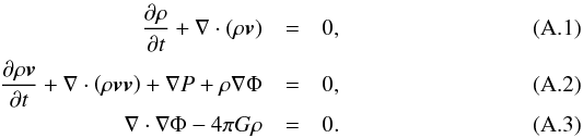 Following Jeans (1902), we supersede these equations with perturbation terms in the x direction ρ = ρ0 + δρ, P = P0 + δP, Φ = Φ0 + δΦ and v = v0 + δv with δv = (δv,0,0)T, linearizing the equations and setting
  , i.e.
 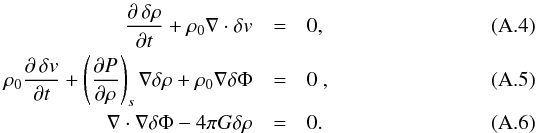 This system of partial differential equations is transformed to an algebraic system of linear equations in the Fourier space: δA = ∫dkÂ(k)exp [i(kx−ωt)], where A represents ρ, v, and Φ. The passage to Fourier space transforms the differential operators ∂/∂t and ∂/∂x to multiplications by −iω and ik, respectively,
 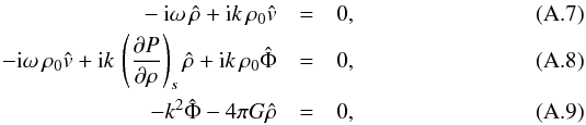 which can be written in matrix form A·x = 0,
 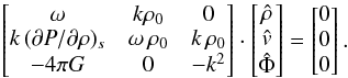 (A.10)Non-trivial solutions for x require that the determinant of A vanishes,
 ![\appendix \setcounter{section}{1} \begin{eqnarray} \det(\matr{A}) = k^2\rho_0 \left[\omega^2 + 4\pi G\rho_0 - k^2 \left({\partial P\over \partial \rho}\right)_s \right] , \end{eqnarray}](/articles/aa/full_html/2016/07/aa26975-15/aa26975-15-eq436.png) (A.11)which is the case for either k = 0, or
(A.11)which is the case for either k = 0, or 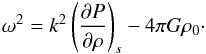 (A.12)A fluid is unstable if ω2< 0, which is the case if
 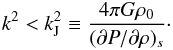 (A.13)
Appendix A.2: Two components
Having two components α and β, the mass and momentum conservation have to be fulfilled for each component as follows: 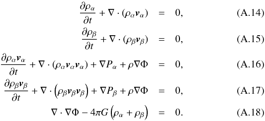 Superseding, as in Appendix A.1, these equations with perturbation terms Aα = Aα0 + δAα and Aβ = Aβ0 + δAβ in the x direction and linearizing them yields
 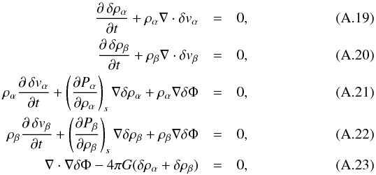 which transform into a linear equation system in Fourier space,
 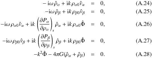 This can be written in the matrix form A·x = 0, defining
  and
and  as follows:
 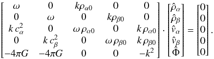 (A.29)In order to simplify, we set Γα = 4πGρα0 and Γβ = 4πGρβ0 and find the following determinant:
 ![\appendix \setcounter{section}{1} \begin{eqnarray} \det(\matr{A}) = k^2 \rho_{\alpha 0} \rho_{\beta 0} \left[\omega^4 + \left(\Gamma_\alpha + \Gamma_\beta - k^2(c^2_\alpha + c^2_\beta)\right)\omega^2 \right.~~~~~~~~~~~~~~~~\nonumber\\ \left.+ k^2\left(-\Gamma_\beta c^2_\alpha - \Gamma_\alpha c^2_\beta + k^2 c^2_\alpha c^2_\beta\right)\right] \ . \end{eqnarray}](/articles/aa/full_html/2016/07/aa26975-15/aa26975-15-eq451.png) (A.30)Again, to have a non-trivial solution, its determinant must be zero, which, in the case of k ≠ 0, is
(A.30)Again, to have a non-trivial solution, its determinant must be zero, which, in the case of k ≠ 0, is 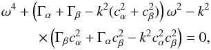 (A.31)with the following solution for ω2:
 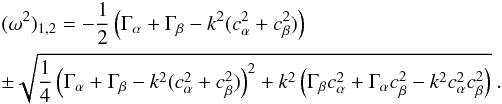 (A.32)Setting ω2 = 0 in Eq. (A.31) yields
 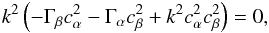 (A.33)with the following solution:
 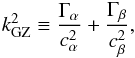 (A.34)a fluid is unstable for ω2< 0 or ω2 ∈ ℑ, which is the case for
  .
.
Appendix A.2.1: Phase transition
In the case of a phase transition, one of the pressure derivatives is equal to zero. Setting cα = 0 in Eq. (A.31) we get ![\appendix \setcounter{section}{1} \begin{eqnarray} \omega^4 + \left[\Gamma_\alpha + \Gamma_\beta -k^2 c^2_\beta\right]\omega^2 -\Gamma_\alpha k^2 c_\beta^2 = 0\label{equ:ompt} , \end{eqnarray}](/articles/aa/full_html/2016/07/aa26975-15/aa26975-15-eq462.png) (A.35)and its solutions is written as
(A.35)and its solutions is written as 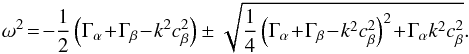 (A.36)Setting ω2 = 0 in Eq. (A.35), only the trivial k = 0 is a solution. Since
  (A.37)the upper sign solution of Eq. (A.36) is always positive and the lower sign solution is always negative for any k. Therefore one ω-solution of Eq. (A.36) is always negative and thus unstable, independent of the strength of either Γα or Γβ.
Appendix B: Energy and radiation transfer during the contraction of a sphere towards an ellipsoid
We consider a non-rotating sphere of radius r initially in unstable equilibrium, which contracts at constant mass as an ellipsoid with semi-principal axes a, b, and c (see Fig. B.1). In a sheet-like collapse, two semi-axes remain the same (a = b = r) while one is decreasing (c = εr), leading to an oblate spheroid. In a filament-like collapse, one semi-axis remains the same (a = r), while two are decreasing together (b = c = εr), leading to a prolate spheroid. In a point-like collapse, all the three semi-axes decrease together (a = b = c = εr), remaining a sphere. During compression, density increases by a factor Z = n/n0. Since the ellipsoid volume is Vell = 4/3 πabc, compression changes as: εoblate = Z-1, εprolate = Z− 1/2, and εsphere = Z− 1/3.
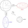 |
Fig. B.1 Collapsing geometries. |
Appendix B.1: Gravitational energy
The gravitational energy difference between the initial sphere and subsequent ellipsoids must be released as additional thermal energy. The gravitational energy of a revolution ellipsoid, with EG,0 = EG,sphere(r) = −(3/5)GM2/r (Landau & Lifshitz 1975), is written as 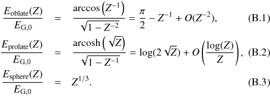 Sheet-like contraction leads to infinite densities with finite temperature increase, which is much more favourable for reaching condensation conditions that filament-like or point-like contractions.
We show now that the maximum relative temperature increase of an initial perfect gas sphere initially in equilibrium is bounded. State 0 is the initial (unstable) equilibrium sphere case, and state 1 is any later, denser case that is not necessarily in equilibrium. Since in equilibrium, the initial state respects the virial condition,  (B.4)where Ekin,0 is the kinetic energy. Since at rest, the initial sphere kinetic energy consists only of microscopic motion, and is proportional to the initial temperature T0.
The initial and later total energies are, 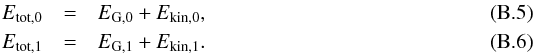 Taking into account possible radiative cooling, we suppose Etot,1 ≤ Etot,0, which leads to, using the initial virial condition,
 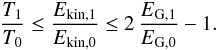 (B.7)The first inequality takes into account that state 1 is not necessarily in equilibrium; some kinetic energy may be attributed to macroscopic motion.
Thus, using the above potential energy ratios, in the case of an oblate spheroid contraction, 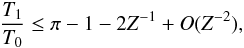 (B.8)that is, the final temperature cannot exceed π−1 ≈ 2.1 times the initial temperature. In the case of a prolate spheroid contraction, temperature is logarithmically bounded as Z increases,
 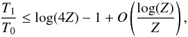 (B.9)while in a spherical contraction, temperature is bounded by the cubic root of compression,
 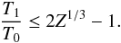 (B.10)
Appendix B.2: Radiative cooling
Energy lost by radiation lowers temperature, but if opacity increases during contraction at some point the radiative cooling rate drops below the heating rate as a result of gravitational energy conversion, thereby slowing down the collapse. Here we show with simple arguments how opacity changes when continuously contracting an initial sphere towards denser, smaller spheres, or towards denser revolution of oblate or prolate kinds of ellipsoids, keeping the longest axes constant and assuming uniform densities at any stage and constant absorption cross sections.
Appendix B.2.1: Optical depth
The optical depth τ in the cumulated absorption over a photon path ℓ:  , where σ is the absorption cross section of individual atoms with number density n. The central optical depth, calculated from the centre to the ellipsoid edge along some direction, is a first order estimator of the average optical depth. We compare the optical depth τ0 = rσn0 for the initial sphere with the later spheres. For revolution ellipsoids, where a and c are the semi-long and short axes, respectively, the distance from the centre to some point on the edge is
 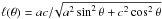 for oblate spheroids and
 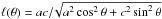 for prolate spheroids. The angle θ vanishes at the spheroid equator. Since the ellipticity ε = c/a varies as Z-1, Z− 1/2, and Z− 1/3 in the oblate, prolate, and spherical cases, respectively, the optical depth ratios as functions of compression Z and θ are found to be
 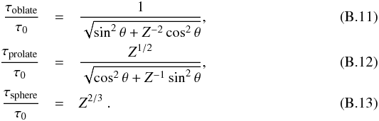 Thus, in the oblate case the central optical depth ratio does not change along the poles and at high compression remains barely increased over most directions. In the prolate case it increases least along the equator, but is proportional to the square root of compression. In the spherical case it increases most rapidly as a power 2/3 of compression. Thus sheet-like compression provides the least optical depth increase and spherical compression compression the most.
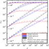 |
Fig. B.2 Absorption probability in contracting spheroids as function of compression Z> 1 calculated by Monte Carlo simulation. At Z = 1 all cases are spherical. The photons start either at the centre only or anywhere inside the ellipsoid in random directions. Different cases are represented where the initial sphere optical depth τ0 is indicated. |
Appendix B.2.2: Global absorption
One can refine the previous estimate for cooling by calculating, for any point inside an ellipsoid, the probability for a photon to be absorbed. For a given optical depth τ the absorption probability is p = 1−exp(−τ). The global probability of absorption must be calculated for all solid angles for all points. These 4- or 5-dimensional integrals for bi- or tri-axial ellipsoids does not seem to be solvable analytically, and straightforward numerical quadratures would be expensive. Thus we resort to a Monte Carlo draw to estimate these quantities. We pick randomly and uniformly a number of points inside the ellipsoid and a random, uniform directional unit vector n, and find the two distances ℓ1, ℓ2, to the edge of the ellipsoid, allowing us to calculate two optical depths τ1, τ2, and the corresponding absorption probabilities p1, p2 for each point. Knowing the starting position x inside the ellipsoid (a,b,c) and the direction vector n, we find the two signed distances to the ellipsoid edge by solving the quadratic equation (x + ℓnx) /a2 + (y + ℓny)2/b2 + (z + ℓnz)2/c2 = 1 for ℓ. Explicitly, noting α = a-2, β = b-2, γ = c-2, for each point x = [x,y,z] the procedure becomes 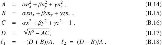 For each set of ℓi, average absorption probabilities can be found for a range of σs. The two absorption probabilities pi = 1−exp(σn | ℓi |), i = 1,2, provide two distinct probabilities for each point. Each set of pis should converge towards a similar average value. The difference allows us to check the error obtained with a finite number of points. Between 2 × 10⁴ (sphere case) and 3 × 10⁷ points (oblate spheroid case) were drawn such that the log 10pi between the two sets differ by at most 0.01. The result is shown in Fig. B.2. The error bars are comparable or smaller than the thickness of the curve.
The sphere and prolate spheroid cases quickly become optically thick, increasing as Z2/3 and Z1/2, respectively, in the optically thin regime. In contrast, the absorption of a contracting optically thin oblate spheroid increases logarithmically until it reaches Zτ0 ~ 1 beyond which it remains approximately constant; in other words if the initial state is optically thin, it remains so even after infinite compression. The emission signature of a collapsing sheet should therefore remain observationally barely noticeable, since both temperature and optical thickness increase by very modest factors in comparison with the other geometries.
Figure 2 shows how an initial sphere at T = 10 K, P = 10-12 Pa would change its temperature and pressure when contracting adiabatically, changing its gravitational energy into thermal energy. Clearly the sheet-like collapse is the most favourable geometry for reaching the H2 phase transition regime. Including radiative cooling, which is the fastest in sheet-like geometry, can only help in this regard.
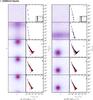 |
Fig. C.1 Time sequence of the simulations A75 and B75. On the left side, the slice shows in depth 20% of the super-molecules. On the right side, Ncomet is the number of super-molecules in one comet and |
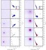 |
Fig. C.2 Time sequence of the simulation B75. On the left side, the slice shows in depth 20% of the super-molecules. On the right side, Ncomet is the number of super-molecules in one comet and |
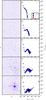 |
Fig. C.3 Time sequence of the simulation C75 with γG = 1.5. On the left side, the slice shows in depth 20% of the super-molecules. On the right side, Ncomet is the number of super-molecules in one comet and |
All Tables
All Figures
|
Fig. 1 H2 (blue) and He (red) phase diagrams. For clarity, only a part of the upper, almost constant density condensed phases of both species and the low-density gas phase of He are shown. |
| In the text | |
|
Fig. 2 H2 and He laboratory data and van der Waals vapour curve derived from Maxwell construct. Adiabatic compression curves of an initial sphere to sheet-, filament- and point-like geometries for interstellar conditions (T = 10 K, P = 10-12 Pa) are shown, as explained in Appendix B. Sheet-like collapses are allowed to reach the phase transition regime even without cooling. Cooling would displaces the curves to lower temperature. |
| In the text | |
|
Fig. 3 van der Waals phase diagram with Maxwell construct for the H2 – He mixture, each species considered as independent. |
| In the text | |
|
Fig. 4 R/cr and A/cavalues as a function of xα for a H2-He mixture. |
| In the text | |
|
Fig. 5 van der Waals phase transition and unvirializable density for a binary mixture with xα = 0.75. |
| In the text | |
|
Fig. 6 Two-dimensional density map of three-dimensional space. |
| In the text | |
|
Fig. 7 Colour mapping of density map. |
| In the text | |
|
Fig. 8 Global temperature as a function of time of the A simulations with γJ = 1.5 and 0.5. |
| In the text | |
|
Fig. 9 Evolution of the number of bound molecules as a function of time of the A), B), and C) simulations with γJ = 1.5 and 0.5. The simulations with γJ = 0.5 are stopped after 5τ, 30τ, and 20τ for the A), B), and C) simulations, respectively, when no further significant development is expected. |
| In the text | |
|
Fig. 10 Density of planetoid as a function of the radius of the simulations A75 and B75 with γJ = 1.5 at t = 5τ and B75 with γJ = 0.5 at t = 30τ. |
| In the text | |
|
Fig. 11 Fraction of bound molecules as a function of time for the simulations A75S with γJ = 1.5 and different Ntot. |
| In the text | |
|
Fig. 12 Fraction of bound β-molecules as a function of Ntot for the simulations A75S. |
| In the text | |
|
Fig. 13 Fraction of bound β-molecules as a function of time for the simulations B75γ. The simulations are stopped once they reach asymptotic values. |
| In the text | |
|
Fig. 14 Fraction of bound molecules with cluster mass mcl>mHe as a function of time of simulations in and out of the unvirializable density domain. |
| In the text | |
|
Fig. 15 Density of planetoid at t = 5τ as a function of the radius of the simulations in and out of the unvirializable density domain. |
| In the text | |
|
Fig. 16 Fraction of bound molecules as a function of time of the simulations B75, B75 with removed β-molecules and B10. γJ = 0.5. |
| In the text | |
|
Fig. 17 γJ of different total fluid masses at T = 10 K, as a function of number density, indicating either ideal gas Jeans instability, or instability owing to phase transition. |
| In the text | |
|
Fig. 18 Snapshots and comet-size distributions of the simulations SSM01, SSM02, and SSE04. The slice selects in depth 20% of the super-molecules. The squares in the two lower left frames are the same size as the next upper frame. |
| In the text | |
|
Fig. 19 Gravitational instabilities at different temperatures and densities for a fluid with Jupiter mass. |
| In the text | |
|
Fig. B.1 Collapsing geometries. |
| In the text | |
|
Fig. B.2 Absorption probability in contracting spheroids as function of compression Z> 1 calculated by Monte Carlo simulation. At Z = 1 all cases are spherical. The photons start either at the centre only or anywhere inside the ellipsoid in random directions. Different cases are represented where the initial sphere optical depth τ0 is indicated. |
| In the text | |
|
Fig. C.1 Time sequence of the simulations A75 and B75. On the left side, the slice shows in depth 20% of the super-molecules. On the right side, Ncomet is the number of super-molecules in one comet and |
| In the text | |
|
Fig. C.2 Time sequence of the simulation B75. On the left side, the slice shows in depth 20% of the super-molecules. On the right side, Ncomet is the number of super-molecules in one comet and |
| In the text | |
|
Fig. C.3 Time sequence of the simulation C75 with γG = 1.5. On the left side, the slice shows in depth 20% of the super-molecules. On the right side, Ncomet is the number of super-molecules in one comet and |
| In the text | |
Current usage metrics show cumulative count of Article Views (full-text article views including HTML views, PDF and ePub downloads, according to the available data) and Abstracts Views on Vision4Press platform.
Data correspond to usage on the plateform after 2015. The current usage metrics is available 48-96 hours after online publication and is updated daily on week days.
Initial download of the metrics may take a while.