| Issue |
A&A
Volume 590, June 2016
|
|
|---|---|---|
| Article Number | A16 | |
| Number of page(s) | 14 | |
| Section | Galactic structure, stellar clusters and populations | |
| DOI | https://doi.org/10.1051/0004-6361/201628274 | |
| Published online | 29 April 2016 | |
A class of spherical, truncated, anisotropic models for application to globular clusters
1
Università degli Studi di MilanoDipartimento di Fisica,
via Celoria 16, 20133
Milano, Italy
e-mail: ruggero.devita@gmail.com
2
University of Surrey, Department of Physics,
Guildford, Surrey
GU2 7XH,
UK
Received: 8 February 2016
Accepted: 14 March 2016
Recently, a class of non-truncated, radially anisotropic models (the so-called f(ν)-models), originally constructed in the context of violent relaxation and modelling of elliptical galaxies, has been found to possess interesting qualities in relation to observed and simulated globular clusters. In view of new applications to globular clusters, we improve this class of models along two directions. To make them more suitable for the description of small stellar systems hosted by galaxies, we introduce a “tidal” truncation by means of a procedure that guarantees full continuity of the distribution function. The new fT(ν)-models are shown to provide a better fit to the observed photometric and spectroscopic profiles for a sample of 13 globular clusters studied earlier by means of non-truncated models; interestingly, the best-fit models also perform better with respect to the radial-orbit instability. Then, we design a flexible but simple two-component family of truncated models to study the separate issues of mass segregation and multiple populations. We do not aim at a fully realistic description of globular clusters to compete with the description currently obtained by means of dedicated simulations. The goal here is to try to identify the simplest models, that is, those with the smallest number of free parameters, but still have the capacity to provide a reasonable description for clusters that are evidently beyond the reach of one-component models. With this tool, we aim at identifying the key factors that characterize mass segregation or the presence of multiple populations. To reduce the relevant parameter space, we formulate a few physical arguments based on recent observations and simulations. A first application to two well-studied globular clusters is briefly described and discussed.
Key words: globular clusters: general / stars: kinematics and dynamics / globular clusters: individual: NGC 104 (47 Tuc) / globular clusters: individual: NGC 5139 (ωCen)
© ESO, 2016
1. Introduction
As a zeroth-order dynamical description, a class of models (King 1966) has long and successfully been applied to globular clusters (McLaughlin & van der Marel 2005; Carballo-Bello et al. 2012; Miocchi et al. 2013). Standard spherical King models are meant to describe round, non-rotating stellar systems made of a single stellar population for which the role of internal two-body relaxation has had time to act, bringing the system close to a quasi-Maxwellian, isotropic distribution function; a truncation is considered, to mimic the presence of tidal effects. The success of the King models is largely based on their ability to fit the observed photometric profiles (but see McLaughlin & van der Marel 2005, for a photometric test in favour of models characterized by a milder truncation); the models are then used to infer the general internal kinematical structure of globular clusters, which is largely beyond the reach of direct observational tests. In recent years, with the advent of high-resolution space and ground-based observations, the great progress made in the acquisition of detailed information on the line of sight and proper motion kinematics of these stellar systems has prompted a demand for more complex dynamical models. In particular, many galactic globular clusters are known to be characterized by significant rotation (Bellazzini et al. 2012; Bianchini et al. 2013) and/or pressure anisotropy (Watkins et al. 2015). Often, clusters that are known to be characterized by longer relaxation times turn out to be more anisotropic (see for example Zocchi et al. 2012, hereafter ZBV12; Watkins et al. 2015).
Regardless of their success, King models exhibit several internal inconsistencies. The models are meant to describe tidally truncated stellar systems, but in their original form they are spherical in spite of the stretching that tides are expected to impose. The models are chosen to reflect the conditions of a collisionally relaxed state, but actually, outside their half-mass radius, globular clusters and the models themselves are associated with very long relaxation times (Harris 2010). These models are generally applied as one-component models, that is, they are suited to describe stellar systems made of a single homogeneous stellar population; yet, if collisional relaxation is at work, it should generate significant mass segregation with heavier stars characterized by a distribution more concentrated than that of lighter stars (Spitzer 1969).
Physically motivated models that are able to resolve some of the above-noted inconsistencies, in relation to the shape and rotation of globular clusters, have been constructed (in particular, see Heggie & Ramamani 1995; Bertin & Varri 2008; Varri & Bertin 2012). As to the possible presence of pressure anisotropy, for the case of non-rotating clusters, so far most studies have resorted to the so-called Michie-King models (Michie 1963), which introduce significant radial pressure in the outer parts by multiplication of the underlying distribution function by a suitable angular-momentum-dependent factor (see also the models recently proposed by Gieles & Zocchi 2015). In this general picture, we might then consider models, such as those known as the f(ν) models, developed to represent the final state of collisionless collapse under incomplete violent relaxation and successfully applied to the study of bright elliptical galaxies (e.g. see Trenti & Bertin 2005). Even though it remains to be proved that the formation of globular clusters, or at least of some globular clusters, follows this route, some recent investigations have looked into this possibility.
A general trend in the direction of radial pressure in the outer regions has also been noted in recent simulations of the evolution of globular clusters (Tiongco et al. 2016). Eventually, if external tidal fields are present, theoutermost regions of the cluster may be characterized by isotropy or mildtangential anisotropy, as also suggested by Vesperini et al. (2014). In a recent paper (ZBV12), the class of spherical f(ν) models was used to study a sample of Galactic globular clusters under differentrelaxation conditions and compared to the performance of the standard spherical King models. This exploratory investigation indicates that for some clusters the use of f(ν) models is encouraged, although because these models are non-truncated, they are obviously at a disadvantage in describing the outer parts of the available photometric profiles. In addition, some of the best-fit radially anisotropic models thus identified actually turn out to be too anisotropic, so that they might be prone to the radial-orbit instability (and thus not acceptable for interpreting the observations). The first goal of the present paper is to introduce a truncation to the f(ν) models and to test whether this new class of models is capable of a more satisfactory fit to the sample of globular clusters studied by ZBV12.
The second objective of the paper is to extend the newly constructed
 models to the case of two-component systems.
For globular clusters, there are at least two important reasons to address more complex
models of this kind.
models to the case of two-component systems.
For globular clusters, there are at least two important reasons to address more complex
models of this kind.
One of the main effects related to collisionality is that of mass segregation. Thus a more realistic dynamical framework for the modelling of globular clusters has been sought in terms of multi-component models (e.g. see Da Costa & Freeman 1976; Gunn & Griffin 1979; Merritt 1981; Miocchi 2006), which basically represent an extension of the standard King (or Michie-King) models. Naively (i.e. in the normal context of kinetic systems), we would expect collisions to enforce a sort of equipartition, in which the velocity dispersion σ of stars of mass m should scale as σ ~ m− 1 / 2. The process is complicated by the global and inhomogeneous nature of self-gravitating systems. It has also been argued that in the core of globular clusters complete equipartition cannot be achieved as a result of the so-called Spitzer instability. In particular, Spitzer (1969) suggested that, in a two-component system in virial equilibrium, the condition of equipartition in the core is precluded if the total mass of the heavy stars exceeds a certain fraction of the total mass of the cluster. Spitzer’s criterion was extended by Vishniac (1978) to cover systems with a continuous distribution of masses. These theoreticalarguments have been revisited by means of recent simulations (see Trenti & van der Marel 2013) in which only partial equipartition is “observed” to follow from the cumulative action of star-star collisions. In any case, a certain degree of mass segregation appears to emerge from the observations of several globular clusters (see Anderson & van der Marel 2010; Goldsbury et al. 2013; Di Cecco et al. 2013; Bellini et al. 2014).
A second, physically separate reason to address the issue of two-component models is given by the relatively recent finding that globular clusters host multiple stellar populations. In many observed cases, the suggested interpretation is that clusters have been the site of multiple generations of stars (see Lardo et al. 2011; Gratton et al. 2012), so that the stars can be divided into the groups of first and second generations, and these groups may be associated with different dynamical properties, such as concentration or degree of anisotropy (see Richer et al. 2013; Bellini et al. 2015).
For the second goal of the paper, that is, the construction of two-component models of the
form, we formulate some physical hypotheses
(based on observations and/or simulations) that correspond to the picture of mass
segregation to keep the number of free parameters low. A comparison with observed cases
should be able to support or disprove the physical assumptions made in the modelling
procedure. Our approach is complementary to that of constructing multi-parameter models as
diagnostic tools (see Da Costa & Freeman 1976;
Gunn & Griffin 1979; Gieles & Zocchi 2015).
The paper is organized as follows. In Sect. 2 we
introduce and construct the new class of truncated anisotropic
models. In Sect. 3 we extend it to the two-component case. In Sect. 4 we apply the one-component models to fit a sample of 13 galactic
globularclusters. For NGC 5139 (ω Cen) and NGC 104 (47 Tuc), we also present the
results of the fits performed by means of two-component
models. Finally, in Sect. 5, we draw our conclusions.
2. One-component models
Studies of the dynamics of elliptical galaxies have investigated the picture of galaxy
formation by incomplete violent relaxation from collisionless collapse. There are ways to
translate this picture into an appropriate choice of the relevant distribution function to
represent the current state of ellipticals. The choice is not unique and various options
have been explored. One particular choice reflects a conjecture on the statistical
foundation of the relevant distribution function (see Stiavelli & Bertin 1987). This is a family of partially relaxed models. The
models are called f(ν) models and their
properties have been studied extensively in more recent papers (see Bertin & Trenti 2003; Trenti et al.
2005). They are based on the following distribution function: ![\begin{equation} \label{fnuDF} f^{(\nu)} = A \exp{\left[-a E - d\left(\frac{J^2}{|E|^{3/2}}\right)^{\nu/2} \right]}, \end{equation}](/articles/aa/full_html/2016/06/aa28274-16/aa28274-16-eq9.png) (1)where A, a, and d are positive constants. For
applications, a given value of ν
≈ 1 is usually taken as a fixed parameter. Here E = v2/ 2 +
Φ(r) < 0 and J = | r ×
v | represent the specific energy and
the magnitude of the specific angular momentum of a single star subject to a spherically
symmetric mean potential Φ(r). The self-consistent models based on this
distribution function define a family of anisotropic, non-truncated models. The following
subsections are devoted to the formulation of a truncated distribution function as a
generalization of Eq. (1)and to the analysis
of the main dynamical properties found for the resulting new classes of anisotropic
truncated models.
(1)where A, a, and d are positive constants. For
applications, a given value of ν
≈ 1 is usually taken as a fixed parameter. Here E = v2/ 2 +
Φ(r) < 0 and J = | r ×
v | represent the specific energy and
the magnitude of the specific angular momentum of a single star subject to a spherically
symmetric mean potential Φ(r). The self-consistent models based on this
distribution function define a family of anisotropic, non-truncated models. The following
subsections are devoted to the formulation of a truncated distribution function as a
generalization of Eq. (1)and to the analysis
of the main dynamical properties found for the resulting new classes of anisotropic
truncated models.
2.1. Truncation
As also noted by Davoust (1977), the truncation
prescription is not unique; the structural properties associated with different types of
truncation are described by Hunter 1977). Indeed,
the distribution functions considered in that article differ from one another for the
smoothness of their energy gradients in correspondence with the energy cut-off. In this
respect, we decided to proceed to the truncation of the f(ν) models with
ν = 1 in
the following way. The distribution function ![\begin{equation} \label{fnuTDF} f_{\rm T}^{(\nu)} = \begin{cases} A \exp{\left[-a(E-E_{\rm e})- \frac{{\rm d}J}{|E-E_{\rm e}|^{\frac{3}{4}}} \right]} & {\rm if}\quad E<E_{\rm e}\\ 0 & {\rm if}\quad E\ge E_{\rm e} \end{cases} \end{equation}](/articles/aa/full_html/2016/06/aa28274-16/aa28274-16-eq18.png) (2)for J ≠ 0, vanishes at the
cut-off energy Ee together with all its derivatives (the
quantities A,Ee,a,
and d are
constants). The two-parameter family of one-component models is then constructed by
solving the Poisson equation
(2)for J ≠ 0, vanishes at the
cut-off energy Ee together with all its derivatives (the
quantities A,Ee,a,
and d are
constants). The two-parameter family of one-component models is then constructed by
solving the Poisson equation  (3)for the gravitational potential
Φ(r). In
our case, the distribution function is anisotropic, so that the density on the right-hand
side of Eq. (3)can be reduced to a
two-dimensional integral, which depends on radius, explicitly and implicitly, through the
unknown Φ(r).
Thus, if we define dimensionless quantities such as the potential ψ = −a(Φ −
Ee), radius ξ = a1 /
4dr, and velocity ω2 = (a/
2)v2, the integral is proportional to
(3)for the gravitational potential
Φ(r). In
our case, the distribution function is anisotropic, so that the density on the right-hand
side of Eq. (3)can be reduced to a
two-dimensional integral, which depends on radius, explicitly and implicitly, through the
unknown Φ(r).
Thus, if we define dimensionless quantities such as the potential ψ = −a(Φ −
Ee), radius ξ = a1 /
4dr, and velocity ω2 = (a/
2)v2, the integral is proportional to
 (4)where
 ![\begin{equation} \label{fnuT_om_zeta} \hat{f}_{\rm T}^{(\nu)}(\xi,\psi,\omega,\zeta)=4\sqrt{2}\pi\exp{\left[-\omega^2+\psi-\frac{\sqrt{2}\xi\omega\sin\zeta}{|\omega^2-\psi |^{3/4}}\right]}~, \end{equation}](/articles/aa/full_html/2016/06/aa28274-16/aa28274-16-eq27.png) (5)and ζ is the angle between the
position r and the velocity v of a single
star. The resulting dimensionless form of Eq. (3)is given by
(5)and ζ is the angle between the
position r and the velocity v of a single
star. The resulting dimensionless form of Eq. (3)is given by  (6)where we introduced the dimensionless
parameter γ =
ad2/
(4πGA). This differential equation is integrated under
the boundary conditions ψ(0) =
Ψ and (dψ/
dξ)(0) = 0 out to the truncation radius
ξtr, where the dimensionless potential
vanishes. Hence, the self-consistent problem for the dimensionless potential reduces to a
family of second-order differential equations defined by two structural parameters: the
central dimensionless potential Ψ and γ. We performed the integration of Eq. (6)with an adaptive fourth-order Runge-Kutta
method. At every integration step, the two-dimensional integral on the right-hand side was
computed by means of the Chure routine in the C-package Cuba (see Hahn 2005).
(6)where we introduced the dimensionless
parameter γ =
ad2/
(4πGA). This differential equation is integrated under
the boundary conditions ψ(0) =
Ψ and (dψ/
dξ)(0) = 0 out to the truncation radius
ξtr, where the dimensionless potential
vanishes. Hence, the self-consistent problem for the dimensionless potential reduces to a
family of second-order differential equations defined by two structural parameters: the
central dimensionless potential Ψ and γ. We performed the integration of Eq. (6)with an adaptive fourth-order Runge-Kutta
method. At every integration step, the two-dimensional integral on the right-hand side was
computed by means of the Chure routine in the C-package Cuba (see Hahn 2005).
2.2. The parameter space
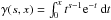
The non-truncated models are characterized by a specific relation between the parameters Ψ and γ (see the plot of γ(Ψ) in Fig. 1 of Trenti & Bertin 2005). In particular, for a given value of Ψ the corresponding value of γ is fixed by the requirement of a Keplerian decay of the gravitational potential (Φ ~ −1 /r) at large radii. For the models with ν = 1, in the range 0 ≲ Ψ ≲ 15, the function γ(Ψ) presents a pronounced peak at Ψ ≈ 5.5; for higher values of Ψ, γ decreases, reaches about half of its peak value at Ψ ≈ 10, and then stays approximately constant.
In our models, γ is left as a free parameter. However, since, for a given Ψ, there is a maximum value γmax beyond which the models do not present any truncation, the parameter space is confined to the region that is under the curve γ(Ψ) found for the non-truncated models. For a given Ψ, the non-truncated models are recovered in the limit γ → γmax; indeed, as shown in Fig. 1, the ratio of the truncation radius rtr to the half-mass radius rM is an increasing function of γ.
The parameter Ψ is identified with the concentration of the model. Another measure of the central concentration is the ratio ρ(0) /ρ(rM) of the central density to the density calculated at the half-mass radius rM. In Fig. 2 we plot this quantity as a function of Ψ. We note that for high values of γ the relation is non-monotonic. For 5.5 ≲ Ψ ≲ 8.5 the relation is monotonic and characterized by a weak dependence on γ .
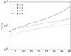 |
Fig. 1 Quantity rtr/rM is plotted as a function of γ for selected values of Ψ. |
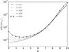 |
Fig. 2 Quantity ρ(0) /ρ(rM) is plotted as a function of Ψ for selected values of γ. |
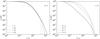 |
Fig. 3 Left panel: normalized density profile for selected values of γ at fixed Ψ; right panel: normalized density profile for selected values of Ψ at fixed γ. |
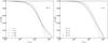 |
Fig. 4 Left panel: normalized total velocity dispersion profile for selected values of γ at fixed Ψ; right panel: normalized total velocity dispersion profile for selected values of Ψ at fixed γ. |
2.3. Intrinsic profiles
All the radial profiles of physical interest can be derived by taking moments of the
distribution function f. If we consider the natural velocity coordinate
system (vr,vθ,vϕ),
the velocity dispersion tensor is diagonal with  . Explicitly, by defining a tangential
component of the velocity dispersion tensor as
. Explicitly, by defining a tangential
component of the velocity dispersion tensor as  , we obtain
 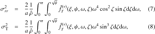 where we have used the definitions given in
Eqs. (4), (5)and the relations:
where we have used the definitions given in
Eqs. (4), (5)and the relations:  and
and
 . For simplicity, in the following we use
the notation
. For simplicity, in the following we use
the notation  . Once the dimensionless potential profile
is obtained by solving the Poisson equation, the velocity dispersion profiles can be
calculated as two-dimensional integrals with the same procedure described in Sect. 2.1.
. Once the dimensionless potential profile
is obtained by solving the Poisson equation, the velocity dispersion profiles can be
calculated as two-dimensional integrals with the same procedure described in Sect. 2.1.
For the one-component models, in Figs. 3 and 4 we plot some intrinsic
profiles of the density and total velocity dispersion (defined by
 ).
).
2.4. Anisotropy
A local measure of the pressure anisotropy is given by the function
 .
.
 |
Fig. 5 Left panel: anisotropy profile α(r) for selected values of γ at fixed Ψ; right panel: anisotropy profile for selected values of Ψ at fixed γ. Where a curve terminates, the truncation radius is reached. |
In Fig. 5 we show some representative anisotropy profiles. The models are characterized by an isotropic core and a radially biased anisotropic envelope.
The radial extent of the isotropic core can be measured by means of the anisotropy radius rα defined as the radius where α = 1.
 |
Fig. 6 Ratio of the anisotropy radius rα to the half-mass radius rM as a function of γ for selected values of Ψ. At given Ψ, models with smaller γ are characterized by a more extended isotropic core. |
 |
Fig. 7 Global anisotropy parameter κ = 2Kr/KT for selected values of the parameter Ψ. The grey area indicates the region of the threshold for the onset of the radial orbit instability. |
The ratio rα/rM of the anisotropy radius to the half-mass radius as a function of γ is shown in Fig. 6. At fixed Ψ, models with higher γ are characterized by lower values of rα/rM.
This trend is confirmed by the behaviour of the ratio κ = 2Kr/KT of twice the total radial kinetic energy Kr to the total tangential kinetic energy KT, which is often used to measure the degree of global anisotropy of the system. This parameter is related to a well-known criterion for the onset of the radial-orbit instability (Polyachenko & Shukhman 1981): instability occurs if κ exceeds a model-dependent threshold, κ ≳ 1.7 ± 0.25. Figure 7 shows the monotonic increasing dependence of κ on γ. Therefore, truncated models are generally more isotropic than the corresponding non-truncated models.
2.5. Virial coefficient
The virial coefficient (for more details see Bertin et al.
2002) can be defined as 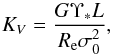 (9)where σ0 is the
“central” velocity dispersion1, Υ∗ is the stellar mass-to-light
ratio in the band used for the determination of the luminosity L, and the effective radius
Re is the projected radius of the disk
containing half of the total luminosity of the cluster.
(9)where σ0 is the
“central” velocity dispersion1, Υ∗ is the stellar mass-to-light
ratio in the band used for the determination of the luminosity L, and the effective radius
Re is the projected radius of the disk
containing half of the total luminosity of the cluster.
Once the best-fit model for a given cluster is found from the photometric fit, the virial coefficient can be calculated, and thus used to infer the total dynamical mass from a measurement of σ0 under the hypothesis of a single stellar component. This procedure is very useful, particularly for those cases in which the kinematic profiles are poor or affected by large uncertainties.
In Fig. 8 we show the value of KV as a function of the central dimensionless potential Ψ for selected values of γ and for the King models. The difference between the various curves can be significant, particularly for low values of Ψ.
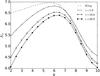 |
Fig. 8 Virial coefficient KV for selected values of γ and for the King models. |
3. Two-component models
Starting from the truncated models described in the previous subsections, we introduce the
two distribution functions ![\begin{equation} \label{fnu2T} f^{(\nu)}_{T,i}(E,J)= \begin{cases} A_i\exp{\left[-a_i(E-E_i)-d_i\frac{J}{\left| E-E_i\right|^{3/4}} \right]} &{\rm if}\quad E<E_i \\ 0 &{\rm if}\quad E\ge E_i. \end{cases} \end{equation}](/articles/aa/full_html/2016/06/aa28274-16/aa28274-16-eq75.png) (10)Each distribution function depends on four
constants Ai,ai,di,Ei
(with i = 1,2),
so that in total the solution for the self-consistent potential Φ from the Poisson equation
(10)Each distribution function depends on four
constants Ai,ai,di,Ei
(with i = 1,2),
so that in total the solution for the self-consistent potential Φ from the Poisson equation 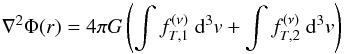 (11)requires a study with eight arbitrary
constants. In practice, from the point of view of dimensionless parameters, we reduce our
investigation to a two-parameter space by means of physical arguments; of course, if
desired, we could loosen some of the physical constraints that we are going to impose and
thus extend our discussion.
(11)requires a study with eight arbitrary
constants. In practice, from the point of view of dimensionless parameters, we reduce our
investigation to a two-parameter space by means of physical arguments; of course, if
desired, we could loosen some of the physical constraints that we are going to impose and
thus extend our discussion.
As noted in the Introduction, different physical arguments can motivate the study of
two-component models. Here we focus on the case in which we distinguish one population of
lighter stars (let m1 be the representative mass of its
individual stars and M1 its associated total mass) from a
second population of heavier stars (with m2>m1 and
in general, M2 ≠
M1), so that the total mass of the cluster
is M =
M1 + M2. As for
the one-component case, we rescale the problem to a dimensionless form, by referring to a
length scale and to an energy scale based on the constants associated with the lighter
component. In particular, we define the dimensionless radius
 and the dimensionless potential
ψ =
−a1(Φ − E1).
After such rescaling, we are left with six independent constants. To reduce the number of
parameters and thus to work in the simplest mathematical context, we make the following
assumptions:
and the dimensionless potential
ψ =
−a1(Φ − E1).
After such rescaling, we are left with six independent constants. To reduce the number of
parameters and thus to work in the simplest mathematical context, we make the following
assumptions:
We consider a common truncation radius, that is, we take
 (12)Such assumption is frequently made as a
starting point for the construction of multi-mass models (e.g. see Da Costa & Freeman 1976).
(12)Such assumption is frequently made as a
starting point for the construction of multi-mass models (e.g. see Da Costa & Freeman 1976).
We consider two-component models in which the total masses associated with the two
components are in a given ratio M1/M2.
Reasonable values for this ratio are suggested by models of the evolution of stellar
populations, as briefly described in Appendix A.
Obviously, this can be seen as a requirement on the ratio of the normalization factors
A1/A2. In
practice, for a globally self-consistent model this constraint can be written as
 (13)(for the notation
 ,
see Eq. (4)). For a desired mass ratio, the equation is basically a relation for the
constant
,
see Eq. (4)). For a desired mass ratio, the equation is basically a relation for the
constant  in terms of
 , but the precise relation has to be worked
out iteratively from the global solution.
, but the precise relation has to be worked
out iteratively from the global solution.
We choose a given value for the single-mass ratio m1/m2;
reasonable values for this ratio are suggested by stellar-population models, as described in
Appendix A. We impose partial energy equipartition in
the central regions of the system by means of the dimensionless parameter η = 0.2. The definition of
η is given a
few lines below. The way in which equipartition is incorporated is not unique (e.g. see
Kondratev & Ozernoi 1982). In its simplest
form, as proposed by Da Costa & Freeman (1976),
energy equipartition is sometimes imposed by means of a relation between the energy scales
of the form a2/a1 =
m2/m1. We
prefer to follow the argument of Miocchi (2006),
which recognizes that equipartition is best ensured in the central, more relaxed regions. On
the other hand, given the support of recent observations (see Bellini et al. 2014) and simulations (see Trenti
& van der Marel 2013), it may be wiser to refer to only partial equipartition,
by imposing ![\begin{equation} \left[\frac{a_2}{a_1}\frac{\gamma\left(5/2,\Psi\right)\gamma\left(3/2,a_2\Psi/a_1 \right)}{\gamma\left(3/2,\Psi\right)\gamma\left(5/2,a_2\Psi/a_1 \right)}\right]^{1/2}= \left(\frac{m_1}{m_2}\right)^{-\eta}\cdot\label{eta} \end{equation}](/articles/aa/full_html/2016/06/aa28274-16/aa28274-16-eq98.png) (14)The left-hand side of the above equation
represents the ratio σ1(0) /σ2(0)
of the central velocity dispersions for the two-component model2. At r =
0, the one-component distribution function is trivial because the
dependence on J
drops out and Φ = Φ(0), so that
Eq. (14)is expressed in closed form in terms
of the relevant constants and concentration parameter Ψ = −a1 [ Φ(0) −
Ee ]. Full equipartition is denoted by
η = 1 / 2;
from their simulations, also in view of an argument by Spitzer (1969) and Trenti & van der Marel
(2013) suggest η =
0.2 for specific cases. In the following we refer to this case of partial
equipartition (for a recent investigation on energy equipartition in globular clusters, see
also Bianchini et al. 2016).
(14)The left-hand side of the above equation
represents the ratio σ1(0) /σ2(0)
of the central velocity dispersions for the two-component model2. At r =
0, the one-component distribution function is trivial because the
dependence on J
drops out and Φ = Φ(0), so that
Eq. (14)is expressed in closed form in terms
of the relevant constants and concentration parameter Ψ = −a1 [ Φ(0) −
Ee ]. Full equipartition is denoted by
η = 1 / 2;
from their simulations, also in view of an argument by Spitzer (1969) and Trenti & van der Marel
(2013) suggest η =
0.2 for specific cases. In the following we refer to this case of partial
equipartition (for a recent investigation on energy equipartition in globular clusters, see
also Bianchini et al. 2016).
We assume that the radial scales that define the size of the radially biased anisotropic
outer envelope are the same for the two components, that is
 (15)This is only a qualitative argument, meant to
recognize that one of the possible causes of radially biased pressure anisotropy is
incomplete violent relaxation, which is a collisionless relaxation process that acts in the
same way on stars of different masses (see also Gunn &
Griffin 1979). For convenience in the numerical calculation of the models, we
decided to adopt the radial scale da1 / 4 as a proxy for
the radius of transition from isotropic core to anisotropic envelope; by inspecting
one-component and two-component models, we confirm that indeed this scale identifies
approximately the anisotropy radius rα.
(15)This is only a qualitative argument, meant to
recognize that one of the possible causes of radially biased pressure anisotropy is
incomplete violent relaxation, which is a collisionless relaxation process that acts in the
same way on stars of different masses (see also Gunn &
Griffin 1979). For convenience in the numerical calculation of the models, we
decided to adopt the radial scale da1 / 4 as a proxy for
the radius of transition from isotropic core to anisotropic envelope; by inspecting
one-component and two-component models, we confirm that indeed this scale identifies
approximately the anisotropy radius rα.
To summarize, our two-component models depend on eight constants. In practice, by taking a
common truncation radius and a common pressure anisotropy scale for the two components and
by fixing the values of the ratios M1/M2,
m1/m2 (and of
η), the
relations introduced above reduce the number of free constants to four. Two of these are
used to rescale the Poisson equation to a dimensionless form, the remaining two define two
independent dimensionless parameters, so that the parameter space explored by the family of
two-component models considered in the present study is two dimensional. As in the
one-component models, we use the central dimensionless potential Ψ = −a1 [ Φ(0) −
Ee ] and the parameter
 as independent structural parameters.
3.1. Mass segregation
The third condition imposed in the construction of two-component models is meant to
incorporate the role of collisions in establishing some sort of equipartition. It is well
known that this effect should be accompanied by mass segregation, that is, by a general
trend of the lighter component to exhibit a more diffuse distribution with respect to the
heavier component. In particular, we note that for our models the central density ratio is
given by  (16)which, under the conditions listed in the
previous subsection, would be expected to fall below unity from a simple picture of mass
segregation in which the central parts should be dominated by the heavier component.
(16)which, under the conditions listed in the
previous subsection, would be expected to fall below unity from a simple picture of mass
segregation in which the central parts should be dominated by the heavier component.
As we noted in Sect. 2.2, when we introduced the concentration parameter Ψ for the one-component models, there are several ways of describing the concentration of a given density profile. Here, we illustrate the result of different definitions that may be adopted. In Fig. 9 we plot the ratio rM1/rM2 of the half-mass radii of the two components and the ratio of the quantities associated with the parameter illustrated in Fig. 2, that is, of the density contrast of the lighter component ρ1(0) /ρ1(rM1) to that of the heavier component ρ2(0) /ρ2(rM2), as a function of Ψ, for selected values of γ. The ratio rM1/rM2 exceeds unity for all the models considered and thus it is the more natural parameter to be used to describe the relative concentration of the two components.
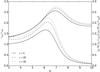 |
Fig. 9 Relative concentration of the two components as a function of Ψ, for selected values of γ. The upper set of curves represents the ratio rM1/rM2 of the half-mass radius of the lighter component to the half-mass radius of the heavier component. The lower set represents the ratio of the density-contrast parameters. |
In order to highlight how different types of mass segregation can result from the condition of partial energy equipartition imposed on our models, we report the cases of two selected globular clusters: 47 Tuc and ω Cen. We found the two-component dynamical models that best reproduce the observed photometric and kinematic profiles of the two clusters. In Fig. 10 we plot the density profiles of the two best-fit models found by the procedure in which red giant stars are not included among the heavy stars (for a discussion of this fitting procedure, see the next section). The best-fit model of 47 Tuc is characterized by a density profile with a larger density of heavy stars in the central regions. Indeed, this is the type of mass segregation traditionally associated with the tendency of the system to establish energy equipartition. The model of ω Cen exhibits a qualitatively different mass distribution.
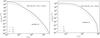 |
Fig. 10 Left panel: density profiles of each component and the total density profile for the best-fit model of 47 Tuc (NGC 104), obtained by the procedure in which RG stars are not included in the heavy component (see text); right panel: corresponding density profiles for the best-fit model of ω Cen (NGC 5139). |
In the next section, devoted to setting the correspondence between dynamical models and observations, we briefly describe how mass segregation has a counterpart in the gradient of the profile of the cumulative mass-to-light ratio, which is defined as the total mass-to-light ratio for a sphere of given radius r.
4. Fitting the data with dynamical models
We performed a combined photometric and kinematic fit to the data available for a set of
globular clusters, following a procedure very similar to that used in ZBV12. In the present analysis we decided to minimize a combined
chi-square function, which is defined as the sum of the photometric and kinematic
contributions. In constrast to the fits reported in ZBV12 by means of one-component non-truncated f(ν) models, the fits
presented here, based on the models, are characterized by one additional
parameter (γ)
strictly connected with the truncation.
4.1. The issue of the mass-to-light ratios
4.1.1. Mass-to-light ratios for one-component models
In the application of one-component models, we follow the general assumption that a constant mass-to-light ratio adequately describes the stellar population that we imagine is homogeneous. This assumption allows us to convert projected mass densities Σ(R) into surface luminosity densities l(R) by means of a simple relation of proportionality. Then, the mass-to-light ratio is found as one of the parameters determined by the fit (see Appendix B of ZBV12).
4.1.2. Mass-to-light ratios for two-component models
In general, for the two-component models we consider the surface luminosity profile as
the sum of the following two contributions: 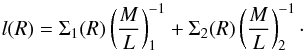 (17)
(17)
Then, we performed two different types of fit:
In the first procedure, we consider the heavier componentmade of only dark remnants. Therefore, the fit is similar to that forelliptical galaxies in the presence of a dark matter component. Inother words, the photometric fit is carried out by omitting theΣ2-term in Eq. (17). Then the kinematic fit is performedby considering only the velocity dispersion profile relative to thelighter component, which is the only component assumed to bevisible.
In the second type of fit, we include red giant stars (RGs) in the group of heavier stars (see Appendix A). In this case, both components contribute to the surface brightness in the photometric fit . Thus, we explored two possible options: either (a) to assign a reasonable value for the ratio (M/L)1/ (M/L)2, based on the fraction of luminosity expected to come from the RGs and main-sequence stars present in the system; or (b) to leave the mass-to-light ratio of the heavier component to be determined as a parameter of the best-fit model, and thus to make a prediction on the number of RGs contained in the system. We report only the results given by option (a), as the best-fit models found with the other option tend to underestimate the contribution of RGs present in globular clusters3. In this procedure the kinematic fit considers the heavier component as the kinematic tracer because most kinematic data come from spectroscopic observations of RGs (i.e. the line-of-sight velocities of RG stars are usually those that are detected for the construction of the observed velocity dispersion profiles).
For the two-component models, the conversion from density profiles to luminosity profiles is not as straightforward as in the one-component case because it depends on the structural characteristics of the system. In particular, it reflects the interconnection between mass segregation and the gradients of mass-to-light ratios. In Fig. 11, we plot the cumulative mass-to-light ratio for two selected globular clusters in their central regions; the behaviour of this quantity as a function of the intrinsic radius r changes according to the type of fit considered. On the one hand, in the case in which RGs are not included in the heavier component, the ratio M/L decreases with r (for the more relaxed cluster 47 Tuc, this trend is more evident). On the other hand, the case in which RGs are included in the heavier component (and in the fitting procedure) is characterized by a mild increase of the cumulative mass-to-light ratio. For the former case, we recover a behaviour of the cumulative mass-to-light ratio profile similar to that found by van den Bosch et al. (2006) for the globular cluster M15 (NGC 7078); they suggest that the gradient of the ratio M/L at small radii is likely to be due to the presence of a centrally concentrated population of dark remnants, an interpretation that is also suited to describe the result of our fit.
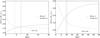 |
Fig. 11 Cumulative mass-to-light ratio as a function of the intrinsic radius r for the best-fit models of two globular clusters. The best-fit models are found by means of two different procedures, that is, by taking the heavier component as made of only dark remnants or by including in the heavier component the presence of red giants. The vertical lines indicate the position of the total half-mass radius. |
We wish to emphasize that in this paper we are not aiming at providing improved dynamical models for selected clusters. Rather, we wish to demonstrate, by means of the mathematically simplest framework, how different ways of using a multi-component dynamical model actually lead to different pictures of the internal structure of globular clusters, especially in relation to mass segregation and gradients of mass-to-light ratios.
4.2. Fits with one-component models
The data sets that we consider are the same as used by ZBV12.
Selected sample of globular clusters.
For convenience, in Table 1 we report some distinctive quantities for the sample of 13 Galactic GCs selected for this paper.
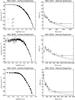 |
Fig. 12 Photometric and kinematic fits for three globular clusters of the sample. Each
cluster is representative of its relaxation class as identified by the core
relaxation time Tc (for NGC 6341, log Tc ≈
7.96; for NGC 6656, log Tc ≈ 8.53; for NGC 2419
log Tc ≈
9.87). The curves represent the surface brightness profile
(left panels) and velocity dispersion profile (right
panels) calculated by means of dynamical models. In particular, dotted
lines correspond to King models; dashed lines to non-truncated f(ν) models, and
solid lines to |
In Fig. 12 we show the best-fit surface brightness and velocitydispersion profiles for three of the selected GCs, which are shown in order of increasing core relaxation time. The dimensionless parameters of the fits and the values of the reduced chi-squared are listed in Table 2. For the statistical analysis we followed the procedure used by ZBV12. From an inspection of the way the best-fit models are identified, we note that the present models are characterized by significant degeneracy in parameter space; this is a natural consequence of the introduction of the additional parameter related to the truncation.
In general, the photometric fits by the  models are more satisfactory than those
performed by means of the King and f(ν) models, for every
relaxation class considered (for a comparison of the values of the reduced chi-squared,
see Table 4 in ZBV12); indeed, for the majority of
the clusters, the minimum chi-squared is inside the 90% confidence interval. The improvement
with respect to the King and f(ν) models is mainly
related to the outer regions of the system, where the truncation of our models
accommodates the observed brightness profiles well.
models are more satisfactory than those
performed by means of the King and f(ν) models, for every
relaxation class considered (for a comparison of the values of the reduced chi-squared,
see Table 4 in ZBV12); indeed, for the majority of
the clusters, the minimum chi-squared is inside the 90% confidence interval. The improvement
with respect to the King and f(ν) models is mainly
related to the outer regions of the system, where the truncation of our models
accommodates the observed brightness profiles well.
In addition, the general trends found by ZBV12 for the non-truncated models are not significantly affected by the truncation. In particular, our models remain able to reproduce the central peak in the velocity dispersion profiles that is characteristic of the least relaxed clusters in the sample (NGC 2419 and NGC 5139).
Best-fit parameters for the one-component models.
Derived physical parameters from the best-fit one-component models.
In Table 3 we report the values of the truncation radius rtr, the projected core radius Rc (that is the radial location where the surface brightness equals half its central value), and the intrinsic half-mass radius rM. Then we list other relevant quantities, in particular, the total mass M, the central density ρ0, and the V-band mass-to-light ratio (M/L)V. For our anisotropic models, we also calculated the intrinsic anisotropy radius rα defined as the radius where α(rα) = 1 and the global anisotropy parameter κ (see Sect. 2.4).
Dimensionless best-fit parameters for the two-component models.
Derived physical parameters from the best-fit two-component models.
4.2.1. A comparison with the King models
No systematic trends are found. The only exception is represented by the truncation
radius, which is generally larger for the models, in line with the general finding
that the photometric profiles appear to possess a smoother truncation than that of King
models (see McLaughlin & van der Marel 2005).
4.2.2. Radial-orbit instability
One of the points noted in the analysis by ZBV12 is a general concern about the possible occurrence of the radial-orbit instability. Polyachenko & Shukhman (1981) argued that this instability would occur when the anisotropy parameter κ = 2Kr/KT, which is the ratio of the radial contribution to the tangential contribution to the total kinetic energy, exceeds 1.7 ± 0.25.
In this respect, for some of the globular clusters considered by ZBV12 (e.g. NGC 6254) the non-truncated f(ν) models might not
be applicable. The truncation in our models tends to reduce the global value
of the radial contribution to the kinetic energy (see Fig. 7), bringing κ down to values typically associated with
stability. Of course, a test by N-body simulations would be desired to confirm
this point, but obviously this would bring us well beyond the goals of the present
paper.
4.3. Fits with two-component models
As anticipated in the previous sections to address the issue of mass segregation in the simplest mathematical framework, we studied the performance of our two-component models in fitting two globular clusters characterized by different relaxation conditions: 47 Tuc (NGC 104) and ω Cen (NGC 5139).
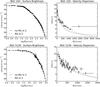 |
Fig. 13 Photometric and kinematic fits for NGC 104 and NGC 5139. The curves represent the surface brightness profile (left panels) and velocity dispersion profile (right panels) calculated by means of two-component models in two ways: taking the heavier component as made of only dark remnants or including the presence of RGs in the heavier component. |
The photometric and kinematic fits for these clusters are presented in Fig. 13. The fits are performed by means of the two procedures outlined in Sect. 4.1. In particular, for the procedure in which RGs are included in the heavier component, we assumed that RGs contribute 60% of the total luminosity of the cluster in the V band. As in the previous subsection, we report the best-fit parameters (see Table 4) and some relevant physical quantities (see Table 5).
The two-component models appear to provide good fits to the observed profiles, thus supporting the hypotheses imposed in their construction. For both clusters the fits performed with the procedure that includes RG stars in the heavier component appear to be better. This is particularly evident for the case of 47 Tuc, for which the best-fit model corresponding to the case without RGs in the heavier component does not adequately reproduce the kinematic profile. We then argue that the role of the stars used as kinematic tracer becomes important when we consider more relaxed environments. In turn, the fit to ω Cen suggests that its stellar population is reasonably homogeneous and mass segregation is probably negligible.
5. Conclusions and perspectives
In this paper we constructed a new class of truncated anisotropic models as an extension of
the so-called f(ν) models introduced
by Stiavelli & Bertin (1987) to describe
elliptical galaxies interpreted as the result of incomplete violent relaxation. We applied
such models to perform a combined photometric and
kinematic study of a sample of Galactic globular clusters.
In the first part of the paper, we constructed one-component truncated models to describe a
stellar system made of a single homogeneous stellar population. From our analysis, the new
class of models is found to be well suited to describe the globular clusters of a sample
studied earlier. We compared our fits with those performed for the same sample of globular
clusters by ZBV12 by means of King and
f(ν) models. In general,
the new truncated models represent the surface brightness profiles better, especially in the
outer parts of the systems. In addition, the models tend to reproduce the inner parts of the
velocity dispersion profiles better than the King models. As also noted by ZBV12, this is probably related to the role played by
radially biased pressure anisotropy in partially relaxed clusters. In the f(ν) and in
models, such radial anisotropy is a
signature of the process of incomplete violent relaxation, which may have occurred during
the initial stages of the evolution of globular clusters; of course, we should be aware that
other mechanisms may be responsible for radially biased pressure anisotropy. In contrast to
some cases found earlier by application of the non-truncated f(ν) models, the
models identified by the fits appear to be
stable with respect to the radial-orbit instability.
In the second part of the paper, we extended our analysis by constructing a family of two-component models with the aim of characterizing in the simplest way a stellar system made of stars with different masses. In fact, if some collisionality is present, stars of different masses are expected to differ in their dynamical evolution, by exhibiting phenomena associated with equipartition and mass segregation. In particular, we assumed that the stellar system under consideration is made of only dark remnants and main-sequence stars with the possible inclusion of red giant stars. Red giant stars would naturally belong to the component of heavier stars, but obviously differ from the heavy dark remnants from the point of view of their visibility. This raises an interesting modelling problem; that is, the question of the optimal comparison between the two-component models thus constructed and the available photometric and kinematic data. To explore the relevant underlying modelling issues, we tested the new two-component models on two globular clusters characterized by different relaxation conditions. They generally provide satisfactory fits to the observed photometric and kinematic profiles, in particular when RGs are included in the fitting procedure, by considering their contribution as heavy stars to the photometric profile and their role in tracing the kinematics of the clusters. Interestingly, from our two-component models only the more relaxed cluster (47 Tuc) exhibits the signature of mass segregation in a prominent way.
The two-component models that we have introduced address the effects induced by collisionality on stars characterized by different masses. This is only one particular application of two-component models. In the near future, we plan to consider the construction of two-component models aimed at addressing the issue of dark matter in globular clusters and of others able to touch on the issue of the recently observed multiple stellar populations, which are generally thought to represent different episodes of star formation (see Gratton et al. 2012).
Typically, RGs are estimated to provide ≈60% of the total V-band luminosity and ≈0.5% of the total mass of a globular cluster; these values were computed by evolving a set of stars with masses distributed according to the Kroupa IMF by means of the SSE package (Hurley et al. 2000).
We note that this choice violates the Spitzer criterion (see Spitzer 1969).
Acknowledgments
We would like to thank A. L. Varri and D. Heggie for helpful suggestions and M. Trenti for useful conversations about the topics addressed in this paper. We are also grateful to S. Degl’Innocenti and to P. G. Prada Moroni for discussions related to the properties of stellar populations in globular clusters. A.Z. thanks M. Gieles and V. Hénault-Brunet for many interesting discussions. This work was partially supported by the Italian MIUR. A.Z. acknowledges financial support from the Royal Society (Newton International Fellowship).
References
- Anderson, J., & van der Marel, R. P. 2010, ApJ, 710, 1032 [NASA ADS] [CrossRef] [Google Scholar]
- Bellazzini, M., Bragaglia, A., Carretta, E., et al. 2012, A&A, 538, A18 [NASA ADS] [CrossRef] [EDP Sciences] [Google Scholar]
- Bellini, A., Anderson, J., van der Marel, R. P., et al. 2014, ApJ, 797, 115 [NASA ADS] [CrossRef] [Google Scholar]
- Bellini, A., Vesperini, E., Piotto, G., et al. 2015, ApJ, 810, L13 [NASA ADS] [CrossRef] [Google Scholar]
- Bertin, G., & Trenti, M. 2003, ApJ, 584, 729 [NASA ADS] [CrossRef] [Google Scholar]
- Bertin, G., & Varri, A. L. 2008, ApJ, 689, 1005 [NASA ADS] [CrossRef] [Google Scholar]
- Bertin, G., Ciotti, L., & Del Principe, M. 2002, A&A, 386, 149 [NASA ADS] [CrossRef] [EDP Sciences] [Google Scholar]
- Bianchini, P., Varri, A. L., Bertin, G., & Zocchi, A. 2013, ApJ, 772, 67 [NASA ADS] [CrossRef] [Google Scholar]
- Bianchini, P., van de Ven, G., Norris, M. A., Schinnerer, E., & Varri, A. L. 2016, MNRAS, 458, 3644 [NASA ADS] [CrossRef] [Google Scholar]
- Carballo-Bello, J. A., Gieles, M., Sollima, A., et al. 2012, MNRAS, 419, 14 [Google Scholar]
- Da Costa, G. S., & Freeman, K. C. 1976, ApJ, 206, 128 [NASA ADS] [CrossRef] [Google Scholar]
- Davoust, E. 1977, A&A, 61, 391 [NASA ADS] [Google Scholar]
- Di Cecco, A., Zocchi, A., Varri, A. L., et al. 2013, AJ, 145, 103 [NASA ADS] [CrossRef] [Google Scholar]
- Gieles, M., & Zocchi, A. 2015, MNRAS, 454, 576 [NASA ADS] [CrossRef] [Google Scholar]
- Gill, M., Trenti, M., Miller, M. C., et al. 2008, ApJ, 686, 303 [NASA ADS] [CrossRef] [Google Scholar]
- Goldsbury, R., Heyl, J., & Richer, H. 2013, ApJ, 778, 57 [NASA ADS] [CrossRef] [Google Scholar]
- Gratton, R. G., Carretta, E., & Bragaglia, A. 2012, A&ARv, 20, 50 [CrossRef] [Google Scholar]
- Gunn, J. E., & Griffin, R. F. 1979, AJ, 84, 752 [NASA ADS] [CrossRef] [Google Scholar]
- Hahn, T. 2005, Comput. Phys. Comm., 168, 78 [Google Scholar]
- Harris, W. E. 2010, ArXiv e-prints [arXiv:1012.3224] [Google Scholar]
- Heggie, D. C., & Ramamani, N. 1995, MNRAS, 272, 317 [NASA ADS] [Google Scholar]
- Hunter, C. 1977, AJ, 82, 271 [NASA ADS] [CrossRef] [Google Scholar]
- Hurley, J. R., Pols, O. R., & Tout, C. A. 2000, MNRAS, 315, 543 [NASA ADS] [CrossRef] [Google Scholar]
- King, I. R. 1966, AJ, 71, 64 [Google Scholar]
- Kondratev, B. P., & Ozernoi, L. M. 1982, Ap&SS, 84, 431 [NASA ADS] [Google Scholar]
- Kroupa, P. 2001, MNRAS, 322, 231 [NASA ADS] [CrossRef] [Google Scholar]
- Lardo, C., Bellazzini, M., Pancino, E., et al. 2011, A&A, 525, A114 [NASA ADS] [CrossRef] [EDP Sciences] [Google Scholar]
- McLaughlin, D. E., & van der Marel, R. P. 2005, ApJS, 161, 304 [NASA ADS] [CrossRef] [Google Scholar]
- Merritt, D. 1981, AJ, 86, 318 [NASA ADS] [CrossRef] [Google Scholar]
- Michie, R. W. 1963, MNRAS, 125, 127 [NASA ADS] [CrossRef] [Google Scholar]
- Miller, G. E., & Scalo, J. M. 1979, ApJS, 41, 513 [NASA ADS] [CrossRef] [Google Scholar]
- Miocchi, P. 2006, MNRAS, 366, 227 [NASA ADS] [CrossRef] [Google Scholar]
- Miocchi, P., Lanzoni, B., Ferraro, F. R., et al. 2013, ApJ, 774, 151 [NASA ADS] [CrossRef] [Google Scholar]
- Polyachenko, V. L., & Shukhman, I. G. 1981, Sov. Astron., 25, 533 [NASA ADS] [Google Scholar]
- Richer, H. B., Heyl, J., Anderson, J., et al. 2013, ApJ, 771, L15 [NASA ADS] [CrossRef] [Google Scholar]
- Salpeter, E. E. 1955, ApJ, 121, 161 [Google Scholar]
- Spitzer, Jr., L., 1969, ApJ, 158, L139 [NASA ADS] [CrossRef] [Google Scholar]
- Stiavelli, M., & Bertin, G. 1987, MNRAS, 229, 61 [NASA ADS] [Google Scholar]
- Tiongco, M. A., Vesperini, E., & Varri, A. L. 2016, MNRAS, 455, 3693 [NASA ADS] [CrossRef] [Google Scholar]
- Trenti, M., & Bertin, G. 2005, A&A, 429, 161 [NASA ADS] [CrossRef] [EDP Sciences] [Google Scholar]
- Trenti, M., & van der Marel, R. 2013, MNRAS, 435, 3272 [NASA ADS] [CrossRef] [Google Scholar]
- Trenti, M., Bertin, G., & van Albada, T. S. 2005, A&A, 433, 57 [NASA ADS] [CrossRef] [EDP Sciences] [Google Scholar]
- van den Bosch, R., de Zeeuw, T., Gebhardt, K., Noyola, E., & van de Ven, G. 2006, ApJ, 641, 852 [NASA ADS] [CrossRef] [Google Scholar]
- Varri, A. L., & Bertin, G. 2012, A&A, 540, A94 [NASA ADS] [CrossRef] [EDP Sciences] [Google Scholar]
- Vesperini, E., Varri, A. L., McMillan, S. L. W., & Zepf, S. E. 2014, MNRAS, 443, L79 [NASA ADS] [CrossRef] [Google Scholar]
- Vishniac, E. T. 1978, ApJ, 223, 986 [NASA ADS] [CrossRef] [Google Scholar]
- Watkins, L. L., van der Marel, R. P., Bellini, A., & Anderson, J. 2015, ApJ, 803, 29 [NASA ADS] [CrossRef] [Google Scholar]
- Zocchi, A., Bertin, G., & Varri, A. L. 2012, A&A, 539, A65 (ZBV12) [NASA ADS] [CrossRef] [EDP Sciences] [Google Scholar]
Appendix A: Dark remnants, red giants, and main-sequence stars
In the present study, we simplified the discussion of the structure of a system made of stars of different masses by grouping the various stars into two components, light stars of mass m1 (and total associated mass M1) and heavy stars of mass m2 (and total associated mass M2). Real globular clusters are extremely complex because they contain not only stars with basically a continuous spectrum of masses, but also objects, such as binary stars, that fall outside the paradigm of the equations traditionally used in stellar dynamics. The main goal of this appendix is to determine “reasonable” estimates for the mass ratios m2/m1 and M2/M1 to be used in our idealized models, as introduced in Sect. 3.
Most of the objects that are naturally assigned to the heavier component (and collectively should make most of the mass M2) are often called “dark remnants”. In fact, white dwarfs, neutron stars, and black holes are not expected to contribute much to the surface brightness profile of the cluster. In turn, most of the mass M1 is expected to be made of low-mass (typically below 0.5 M⊙) main-sequence stars. There remains a third class of stars, the red giant stars, which are expected to belong to the heavier component (because their mass is thought to be in the range 0.7−0.8 M⊙, very similar to the average mass of the remnants; see below), with only minor contribution to M2; yet, they are expected to contribute significantly to the observed surface brightness and, importantly, are generally used as kinematic tracers in the sense that they are the main source of the kinematic data points collected by spectroscopic observations. The modelling of globular clusters addressed in this paper is thus significantly different from that used in the two-component description of elliptical galaxies, for which one component represents the luminous collisionless stellar system and the other component the dark matter halo; still, an element of analogy exists because in both cases the structural profiles of self-consistent two-component models are generally different from those of one-component models.
To estimate a priori some quantities that define our idealized model, we start from the
initial mass function (IMF), which defines the initial distribution of stars with mass.
Then we make some very simple assumptions about star evolution to estimate how stars have
evolved from their initial condition and thus infer some properties of the present
distribution of masses. We refer to three different IMFs. The first has been proposed by
Salpeter (1955) and is a single power law
 (A.1)where D is a constant. Thus, the
quantity ξ(m)dm is the
initial number of stars with mass in the range (m,m + dm). The total mass of
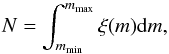
stars within the mass range (mmin, mmax) is given
by a simple integration
(A.1)where D is a constant. Thus, the
quantity ξ(m)dm is the
initial number of stars with mass in the range (m,m + dm). The total mass of
stars within the mass range (mmin, mmax) is given
by a simple integration  (A.2)The corresponding number of stars is
 (A.3)so that a mean value for the single mass is
given by m =
M/N. The other forms of IMF
considered are taken from Miller & Scalo (1979)
and Kroupa (2001).
(A.3)so that a mean value for the single mass is
given by m =
M/N. The other forms of IMF
considered are taken from Miller & Scalo (1979)
and Kroupa (2001).
More massive stars evolve more rapidly, leaving the main sequence and becoming remnants after a relatively rapid transition in the giant branch. For our purposes, we assume that the main-sequence stars with masses larger than ≈0.8 M⊙ become remnants instantly (i.e. in a time very short compared to the age of the cluster). In particular, stars with masses from 0.8 to 10 M⊙ become white dwarfs, those with masses from 10 to 25 M⊙ become neutron stars, and those from 25 to 100 M⊙ end up as black holes (we adopted the same mass ranges used by Gill et al. 2008). A certain fraction of the initial mass is lost through supernova explosions or gas expelled by planetary nebulae. Thus, for white dwarfs we consider masses in the range 0.5−1.4 M⊙; for neutron stars we take masses in the range 1.3−2 M⊙, and for black holes we consider masses in the range 5−10 M⊙. Fast evolution is thus assumed to map an initial range of masses 0.8−100 M⊙ distributed according to the IMF into a present-day mass range 0.5−10 M⊙ for the remnants. The mass functions of the remnants are thus constructed from the IMF by taking the same slope in the corresponding mass ranges. The number of remnants must be equal to the initial number of the main-sequence stars. Such condition fixes the constant D of the mass function of the remnants. Once the various mass functions have been properly defined, we proceed to calculate the mean mass and total mass of each group of objects. The results are summarized in Table A.1.
By identifying the light stars of component 1 with the main-sequence stars and the heavy stars of component 2 with the remnants, in our models we take4, for simplicity, m1 = 0.25 M⊙, m2 = 0.75 M⊙, m2/m1 = 3 and M2/M1 = 1 / 3.
Therefore, the idealized evolution model considered in this appendix does not include the presence of RGs in the final state. A posteriori the presence of RGs may be taken into account by considering the mass-to-light ratio of the heavy component in the idealized two-component models as a parameter depending on the number of RGs present in the cluster. By determining the mass-to-light ratio of the heavy component, a fit to the data could thus give an estimate of the number of giants in the cluster. Alternatively, if an estimate of the number of RGs is available independently, we would have an a priori estimate of the mass-to-light ratio for the heavy component and thus test the adequacy of the two-component models under such a constraint.
Masses of different stellar components.
All Tables
All Figures
|
Fig. 1 Quantity rtr/rM is plotted as a function of γ for selected values of Ψ. |
| In the text | |
|
Fig. 2 Quantity ρ(0) /ρ(rM) is plotted as a function of Ψ for selected values of γ. |
| In the text | |
|
Fig. 3 Left panel: normalized density profile for selected values of γ at fixed Ψ; right panel: normalized density profile for selected values of Ψ at fixed γ. |
| In the text | |
|
Fig. 4 Left panel: normalized total velocity dispersion profile for selected values of γ at fixed Ψ; right panel: normalized total velocity dispersion profile for selected values of Ψ at fixed γ. |
| In the text | |
|
Fig. 5 Left panel: anisotropy profile α(r) for selected values of γ at fixed Ψ; right panel: anisotropy profile for selected values of Ψ at fixed γ. Where a curve terminates, the truncation radius is reached. |
| In the text | |
|
Fig. 6 Ratio of the anisotropy radius rα to the half-mass radius rM as a function of γ for selected values of Ψ. At given Ψ, models with smaller γ are characterized by a more extended isotropic core. |
| In the text | |
|
Fig. 7 Global anisotropy parameter κ = 2Kr/KT for selected values of the parameter Ψ. The grey area indicates the region of the threshold for the onset of the radial orbit instability. |
| In the text | |
|
Fig. 8 Virial coefficient KV for selected values of γ and for the King models. |
| In the text | |
|
Fig. 9 Relative concentration of the two components as a function of Ψ, for selected values of γ. The upper set of curves represents the ratio rM1/rM2 of the half-mass radius of the lighter component to the half-mass radius of the heavier component. The lower set represents the ratio of the density-contrast parameters. |
| In the text | |
|
Fig. 10 Left panel: density profiles of each component and the total density profile for the best-fit model of 47 Tuc (NGC 104), obtained by the procedure in which RG stars are not included in the heavy component (see text); right panel: corresponding density profiles for the best-fit model of ω Cen (NGC 5139). |
| In the text | |
|
Fig. 11 Cumulative mass-to-light ratio as a function of the intrinsic radius r for the best-fit models of two globular clusters. The best-fit models are found by means of two different procedures, that is, by taking the heavier component as made of only dark remnants or by including in the heavier component the presence of red giants. The vertical lines indicate the position of the total half-mass radius. |
| In the text | |
|
Fig. 12 Photometric and kinematic fits for three globular clusters of the sample. Each
cluster is representative of its relaxation class as identified by the core
relaxation time Tc (for NGC 6341, log Tc ≈
7.96; for NGC 6656, log Tc ≈ 8.53; for NGC 2419
log Tc ≈
9.87). The curves represent the surface brightness profile
(left panels) and velocity dispersion profile (right
panels) calculated by means of dynamical models. In particular, dotted
lines correspond to King models; dashed lines to non-truncated f(ν) models, and
solid lines to |
| In the text | |
|
Fig. 13 Photometric and kinematic fits for NGC 104 and NGC 5139. The curves represent the surface brightness profile (left panels) and velocity dispersion profile (right panels) calculated by means of two-component models in two ways: taking the heavier component as made of only dark remnants or including the presence of RGs in the heavier component. |
| In the text | |
Current usage metrics show cumulative count of Article Views (full-text article views including HTML views, PDF and ePub downloads, according to the available data) and Abstracts Views on Vision4Press platform.
Data correspond to usage on the plateform after 2015. The current usage metrics is available 48-96 hours after online publication and is updated daily on week days.
Initial download of the metrics may take a while.