| Issue |
A&A
Volume 590, June 2016
|
|
|---|---|---|
| Article Number | A6 | |
| Number of page(s) | 6 | |
| Section | Stellar atmospheres | |
| DOI | https://doi.org/10.1051/0004-6361/201628266 | |
| Published online | 28 April 2016 | |
Temperatures and metallicities of M giants in the Galactic bulge from low-resolution K-band spectra⋆
1
Laboratoire Lagrange, Université Côte d’Azur, Observatoire de la Côte
d’Azur, CNRS, Bvd de l’Observatoire,
06304
Nice,
France
e-mail:
This email address is being protected from spambots. You need JavaScript enabled to view it.
2
Department of Astronomy and Theoretical Physics, Lund Observatory,
Lund University, Box
43, 221 00
Lund,
Sweden
e-mail:
This email address is being protected from spambots. You need JavaScript enabled to view it.
Received: 7 February 2016
Accepted: 7 March 2016
Abstract
Context. With the existing and upcoming large multifibre low-resolution spectrographs, the question arises of how precise stellar parameters such as Teff and [Fe/H] can be obtained from low-resolution K-band spectra with respect to traditional photometric temperature measurements. Until now, most of the effective temperatures in Galactic bulge studies come directly from photometric techniques. Uncertainties in interstellar reddening and in the assumed extinction law could lead to large systematic errors (>200 K).
Aims. We obtain and calibrate the relation between Teff and the 12CO first overtone bands for M giants in the Galactic bulge covering a wide range in metallicity.
Methods. We used low-resolution spectra for 20 M giants with well-studied parameters from photometric measurements covering the temperature range 3200 <Teff< 4500 K and a metallicity range from 0.5 dex down to −1.2 dex and study the behaviour of Teff and [Fe/H] on the spectral indices.
Results. We find a tight relation between Teff and the 12CO(2−0) band with a dispersion of 95 K and between Teff and the 12CO(3−1) with a dispersion of 120 K. We do not find any dependence of these relations on the metallicity of the star, which makes them attractive for Galactic bulge studies. This relation is also not sensitive to the spectral resolution, which allows this relation to be applied in a more general way. We also find a correlation between the combination of the Na i, Ca i, and the 12CO band with the metallicity of the star. However, this relation is only valid for subsolar metallicities.
Conclusions. We show that low-resolution spectra provide a powerful tool for obtaining effective temperatures of M giants. We show that this relation does not depend on the metallicity of the star within the investigated range and is also applicable to different spectral resolutions making this relation in general useful for deriving effective temperatures in high-extinction regions where photometric temperatures are not reliable.
Key words: stars: fundamental parameters / stars: late-type / Galaxy: bulge / infrared: stars
Based on observations collected at the European Southern Observatory, Chile, program number 089.B-0312B.
© ESO, 2016
1. Introduction
While photometric temperatures can be estimated quite precisely in low-extinction windows (see e.g. González Hernández & Bonifacio 2009), regions where interstellar reddening is high (e.g. Galactic bulge, Galactic plane), photometric temperatures by definition suffer from large and unknown systematic uncertainties. Going even closer to the Galactic centre region (RGC< 200 pc) it is virtually impossible to get reliable photometric temperatures owing to the extreme high interstellar reddening (Schultheis et al. 2009, 2014; Gonzalez et al. 2012). To overcome this problem, Ryde & Schultheis (2015) instead derived Teff from spectral indices in low-resolution K-band spectra in their study of Galactic centre stars. They were then able to obtain accurate detailed chemical abundances of nine M giant stars close to the Galactic centre using the CRIRES high-resolution spectrograph. This technique was extended to latitudes at b = −1° and b = −2° (Ryde et al. 2016).
Ramirez et al. (1997) and Ramírez et al. (2000) studied the behaviour of the 12CO band head situated at 2.3 μm with low-resolution K-band spectra (R ~ 2000−4000) and found for M giants a remarkably tight relation between the equivalent width (EW) and the effective temperature. Blum et al. (2003) and Ivanov et al. (2004) confirmed this strong temperature dependence of the 12CO band head using a different spectral resolution.
Ramírez et al. (2000), Frogel et al. (2001), Schultheis et al. (2003), and Ivanov et al. (2004) found that the combined index of the Nai doublet at 2.21 μm and the Cai triplet at 2.261 μm is very sensitive to the surface gravity of the star and can be used, for example, to distinguish M giants from supergiants or dwarf stars. Schultheis et al. (2003) has shown the power of low-resolution spectra in the region of high interstellar extinction. They were able to distinguish between different stellar populations such as red giant branch stars, asymptotic giant branch stars, supergiants, or young stellar objects. Frogel et al. (2001) and Ramírez et al. (2000) obtained relations between EW(Nai), EW(Cai), and [Fe/H] which were calibrated on globular clusters. Based on this calibration, Ramírez et al. (2000) studied the metallicity distributions in the Galactic centre region and found no evidence of a metallicity gradient for the inner Bulge. Pfuhl et al. (2011) determined the average star formation rate from 450 cool giant stars located in the nuclear star cluster. They obtained low-resolution spectra (R ~ 2000−3000) of 33 giants in the solar neighbourhood (−0.3 < [ Fe / H ] < 0.2) with spectral types from G0–M7 and obtained a CO−Teff relation with a residual scatter of 119 K. However, the Teff vs. 12CO calibration has been only investigated for a bright local solar neighbourhood sample with a narrow metallicity range. We extended this study to M giants located in the Galactic bulge and used a wide metallicity range to test this calibration.
Until now most of the abundance studies (e.g. Rich & Origlia 2012; Gonzalez et al. 2011; Zoccali et al. 2008) in Galactic bulge fields use photometric temperatures based on a colour-temperature relation and assuming interstellar reddening values as a first temperature estimate. However, variable extinction, uncertainties in the extinction law, etc. can lead to severe uncertainties in the derived temperatures (>200 K), which can lead to unknown and different systematic offsets in the abundance determination. Here we apply and investigate these relations for stellar abundances studies in the Bulge, extending their use to a wide range of metallicities
In this paper, we show how low-resolution spectra can be a powerful tool with which to obtain highly accurate effective temperatures in highly extincted regions (such as the Galactic centre). We are able to show that this method chosen by e.g. Ryde & Schultheis (2015) and Ryde et al. (2016), indeed is a good choice. The paper is structured as follows: in Sect. 2 we describe the data and the data reduction process; in Sect. 3 we discuss how the known effective temperature and metallicity of our calibration stars relates with the CO bands and the spectral indices such as Na i and Ca i; in Sect. 4 we apply our method to M giants in the inner Galactic bulge; and we finish in Sect. 5 with the conclusions.
2. Observations
We obtained near-IR spectra on 27 June–30 June 2010 with ISAAC at ESO, Paranal, Chile. We used the red grism of the ISAAC spectrograph, covering 2.0–2.53 μm, to observe 21 M giants in the Galactic bulge. We observed the spectra under photometric conditions through a 1″ slit providing a resolving power of R ~ 2000. We obtained a Ks-band acquisition image before each spectrum to identify the source and place it on the slit. We used UKIDSS finding charts for source identification and to choose empty sky positions for sky subtraction for each source along the 90″ slit. We used an ABBA observing sequence for optimal sky subtraction.
We observed B dwarfs (typically 6−8 stars per night) close to the airmass range of our targets as telluric standard stars to correct for the instrumental and atmospheric transmission. We used IRAF to reduce the ISAAC spectra. We removed cosmic ray events, subtracted the bias level, and then divided all frames by a normalized flat field. We used the traces of stars at two different positions (AB) along the slit to subtract the sky. After extracting and co-adding the spectra, we calibrated wavelengths using the Xe-lamp. The rms. of the wavelength calibration is better than 0.5 Å.
We rebinned the spectra to a linear scale with a dispersion of ~7 Å pixel and a wavelength range from 2.0 μm to 2.51 μm. We then divided each spectrum by the telluric standard observed closest in time and in airmass (airmass difference <0.05). We then normalized the resulting spectra by the mean flux between 2.27 and 2.29 μm. Table 1 shows the list of known Bulge stars with precise stellar parameters. Our stars lie in the temperature range 3200 <Teff< 4500 K and are selected from Rich & Origlia (2005), Rich et al. (2012), Gonzalez et al. (2011a), and Monaco et al. (2011). They span a wide range of metallicities ensuring that we can study a possible metallicity dependance of the CO vs. Teff relation
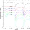 |
Fig. 1 Temperature sequence of the CO bandhead starting from 4500 K (black) going down to 3200 K (cyan) in 200 K steps. The star names are indicated (see Table 1). |
Figure 1 shows the temperature sensitivity of the CO bandhead where we see a steady increase in the absorption band with effective temperature.
2.1. Stellar samples: Calibrators and target M giants
Our sample of stars covers the M giant sample in Baade’s window from Rich & Origlia (2005) and Gonzalez et al. (2011b). All are from low extinction fields where we can trust and account for the reddening in an accurate way. In addition, we include stars from Rich et al. (2012) that are located at l = 0° and b = −1°. This field, which is close to the Galactic centre, shows well-studied interstellar extinction (see e.g. Schultheis et al. 1999; Gonzalez et al. 2012). The other stars come from the thick disc study of Monaco et al. (2011) where the temperatures were obtained by using the dereddened (J − K)0 colour, but with little and well-quantified reddening.
We use our derived calibration based on the stars in Table 1 on a sample of stars in the highly extincted inner Bulge region. Thus to obtain effective temperatures, we have also observed, using the same instrument setup, 28 Bulge M giants within 2 deg of the Galactic centre along the southern minor axis. These 28 stars were also observed with CRIRES in order to get detailed chemical abundances (see Ryde & Schultheis 2015; Ryde et al. 2016). Nine stars were observed in the Galactic centre (Ryde & Schultheis 2015), nine stars at (l,b) = (0, −1°), and ten stars at (l,b) = (0, −2°). These stars are M giants with Teff = 3300−4200 K and 0.7 < log g< 2.25, for which metallicities, [Fe/H], and the abundances of the α elements Mg, Si, and Ca were determined. Table 2 shows the M giant sample of Ryde et al. (2016) together with the derived effective temperatures and metallicities in this work (see Sect. 4) and the metallicities derived in Ryde et al. (2016).
Observed targets together with RA, Dec, K magnitude, spectral type, Teff, log g, and [Fe/H].
3. Method: Empirical temperatures and metallicities
In this section we discuss our method based on our calibration sample (Table 1).
3.1. Effective temperature
When measuring the equilavent width of the 12CO band, the choice of the pseudo-continuum bands is important (see e.g. Ivanov et al. 2004). We tested different continuum bands such as those from Ramírez et al. (2000), Frogel et al. (2001), Ivanov et al. (2004), Pfuhl et al. (2011) and looked for the smallest dispersion in Teff in our sample. We have found that the Blum et al. (2003) bandpasses and continuum points show in general the smallest rms dispersion. The absorption indices defined by Blum et al. (2003) are measured relative to spectral regions adjacent to the absorption itself and are thus independent of reddening. The 12CO(2−0) index is defined as the percentage of the flux in the 12CO(2−0) feature relative to a continuum band centred at 2.284 μm. The 12CO(2−0) band and continuum band is 0.015 μm wide and the 12CO(2−0) band is centred at 2.302 μm (see Blum et al. 2003). In addition, we also measure the 12CO(3−1) bandhead. Table 1 gives central wavelengths and bandpasses for the CO lines and their pseudo-continuum.
Figure 2 shows the 12CO(2−0) index of the Blum et al. (2003) sample and the value of our sample. The black lines give the fitted relation of Blum et al. (2003) with Teff = 4828.0−77.5 × CO(2−0) which is very similar to our linear least-square fit. The rms of the fit is 95 K which is comparable with the rms scatter of Pfuhl et al. (2011).
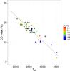 |
Fig. 2 Effective temperature vs. 12CO(2−0) band as a function of metallicity. Black asterisks are the stars from Blum et al. (2003) The straight line shows the fitted relation by Blum et al. (2003). |
The Blum et al. (2003) sample covers bright solar neighbourhood giant stars (see their Table.3) with typical solar metallicities. We extended this work for Galactic bulge stars in low extinction fields covering a wide metallicity range, −1.2 < [ Fe / H ] < 0.5, which enables any possible metallicity dependence of this relation to be tested. As shown in Fig. 2, we do not find any metallicity dependence on this relation within the metallicity range of our calibration stars, relevant for the Bulge, making this method extremely interesting for Galactic bulge studies. The spectral resolution of the comparison stars in Blum et al. (2003) is ~750. As can be seen in Fig. 2, the effect of using a different instrument setup with a different spectral resolution (i.e. R ~ 2000 vs. R ~ 750) does not affect the 12CO(2−0) vs. Teff relation. This also indicates that the CO index is insensitive to spectral resolution and could therefore be used more generally.
Effective temperatures from this work, metallicities from the high-resolution work of Ryde et al. (2016), and metallicities from this work (Col. 4) of the Galactic bulge M giant sample.
Band passes and continuum points of the 12CO bands.
Figure 3 shows a similar plot but using the 12CO(3−1) band centred at λc = 2.3245 μm. We use the same continuum points as for the 12CO(2−0) band (see Table 1). We see here again a very tight relation between Teff and the 12CO(3−1) band. A linear least-square fit gives us this relation with Teff = 4974.85−56.53 × CO(3–1) with an rms of 120 K which is slightly higher than it is for 12CO(2−0). However, both CO band heads are clearly excellent temperature indicators. In addition, we tried to measure the 12CO(4–2) band centred at λc = 2.3535 μm. Although we see clearly, as for the other bands, an increase of the band strength with decreasing temperature, the intrinsic scatter is much higher (~200 K) and so we do not discuss this relation further.
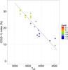 |
Fig. 3 Effective temperature vs. 12CO(3−1) band as a function of metallicity. The straight line shows our best fit. |
How do the spectroscopic temperatures compare with those derived from photometric measurements? Figure 4 shows the comparison between temperatures derived from photometric colours and from spectroscopy for our sample (see Table 1). In order to calculate the photometric temperatures, here we used the temperature scale of M giants from Montegriffo et al. (1998), which is derived from black-body fits of population II stars and those of Houdashelt et al. (2000) using synthetic colours of M giants from MARCS models. We used the dereddened (J − K)0 colour of our stars to obtain the photometric temperatures. The mean difference between Montegriffo et al. (1998) and the temperatures from the 12CO(2−0) index is 10 K ± 200, while for the photometric temperatures of Houdashelt et al. (2000) they are systematically about 90 K higher with a higher rms dispersion ± 250 K.
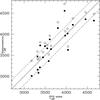 |
Fig. 4 Photometric temperatures vs. spectroscopically derived temperatures. Open circles use the relation by Houdashelt et al. (2000), black circles those from Montegriffo et al. (1998). |
3.2. Metallicity
With the upcoming low-resolution multifibre near-IR spectrographs (MOONS, MOS, etc.), the main question arises of how accurate the metallicities with low-resolution infrared spectra are compared to high-resolution IR spectra. During the last years several studies have been published that trace metallicity distribution functions and metallicity gradients. Gonzalez et al. (2011b) has derived photometric metallicities based on VVV data along the Bulge minor axis where accurate high-resolution spectroscopic metallicities are available. They find a remarkable agreement between the two methods. Gonzalez et al. (2013) has obtained a full low-resolution metallicity map over the VVV Bulge footprint where they revealed a clear metallicity gradient of 0.28 dex/kpc. Owing to the high extinction, this map is restricted to | b | > 3°. Ramirez et al. (1997) have established an [Fe/H] scale for Galactic globular clusters based on medium-resolution (1500−3000) infrared K-band spectra. The technique uses the same absorption features that we use here (Na i, Ca, and CO). The technique was calibrated and tested for globular cluster giants with −1.8 < [ Fe / H ] < −0.1 and −7 < MK< −4 and has a typical uncertainty of ± 0.1 dex. Ramírez et al. (2000) has calculated metallicities for 110 M giants in the inner Bulge using these spectral indices of Na i, Ca, and CO. Schultheis et al. (2003) has applied this technique to obtain the metallicity distribution of ISOGAL sources in the inner degree of our Galaxy. Do et al. (2015) has observed low-resolution K-band spectra (R ~ 5000) of late-type giants within the central 1 pc and obtained metallicities by fitting very sparsely sampled synthetic spectra, intended for calculating MARCS model atmospheres (which should actually not be used as synthetic stellar spectra; see the MARCS homepage1). Their estimated uncertainties are consequently larger than 0.3 dex with some very uncertain systematic effects leading to extremely metal-rich stars.
We used solution 1 from Ramírez et al. (2000), which does not take any photometric quantities into account with the following relation, ![Mathematical equation: \begin{eqnarray} \rm [Fe/H] &=&\, -1.782 + 0.352 \times {\it EW}({\rm Na}) - 0.0231\notag\\& \times {\it EW}({\rm Na})^{2}- 0.0267 \times {\it EW}({\rm Ca}) + 0.0129\notag\\ && \times {\it EW}({\rm Ca})^{2} +0.0472 \notag\\&\times {\it EW}({\rm CO}) - 0.00109\notag \times {\it EW}({\rm CO})^{2}, \end{eqnarray}](/articles/aa/full_html/2016/06/aa28266-16/aa28266-16-eq53.png) where EW(CO), EW(Na), and EW(Ca) are the equilavent widths of CO, Na, and Ca, respectively. Figure 5 shows the comparison of metallicities derived as in Ramírez et al. (2000) from low-resolution spectra and those from high-resolution infrared spectra coming from our calibration sample. We note that there is a general correlation between the metallicities derived from high-resolution IR spectra and those from low-resolution spectra. The dispersion is of the order of ~0.2 dex.
where EW(CO), EW(Na), and EW(Ca) are the equilavent widths of CO, Na, and Ca, respectively. Figure 5 shows the comparison of metallicities derived as in Ramírez et al. (2000) from low-resolution spectra and those from high-resolution infrared spectra coming from our calibration sample. We note that there is a general correlation between the metallicities derived from high-resolution IR spectra and those from low-resolution spectra. The dispersion is of the order of ~0.2 dex.
4. Application of the method to M giants in the Galactic bulge
4.1. Temperature
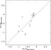 |
Fig. 5 [Fe/H] comparison between low-resolution spectra (Ramirez et al. 2000) and high-resolution spectra from our calibration sample (Table 1). |
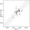 |
Fig. 6 Photometric temperatures vs. spectroscopically derived temperatures for the stars of Ryde et al. (2016). Open circles use the Houdashelt et al. (2000) relation, black circles Montegriffo et al. (1998). Owing to the missing J counterpart, the stars in the Galactic centre (see Table 2) were omitted. |
We applied this method to the M giant sample of Ryde et al. (2016) located in the inner 300 pc of the Milky Way. Figure 6 shows the comparison between our method and photometrically derived temperatures. We see here a more scattered diagram which is due to variable, patchy extinction making the photometric temperatures less reliable. Owing to the extreme high extinction in the Galactic centre region, the M giants of Ryde & Schultheis (2015) do not have J counterparts and are not included in Fig. 6
4.2. Metallicity
Figure 7 shows the application of this method to the M giant Bulge sample of Ryde & Schultheis (2015) and Ryde et al. (2016). We see an increased spread or even a plateau at about [ Fe / H ] = 0.0 for the low-resolution part where the metal-rich stars no longer follow this relation. This indicates that the Na and the Ca lines saturate in the most metal-rich stars. Indeed, by tracing the equilavent width of Na i and Ca i alone, one can see this plateau at around solar metallicity. This means that the proposed relation of Ramírez et al. (2000) is only valid for M giants with subsolar metallicities. Therefore, this metallicity index is not suitable for Galactic bulge studies or for the metal-rich component of the metallicity distribution of Bulge stars, but can be used in low-metallicity systems such as globular clusters or dwarf spheroidals.
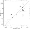 |
Fig. 7 [Fe/H] comparison between low-resolution spectra and high-resolution spectra for the stars from Ryde & Schultheis (2015) and Ryde et al. (2016). |
5. Conclusions
In high extincted regions such as the Galactic bulge and especially the Galactic centre, the precision in the photometric temperatures and gravities are hampered by the poor knowledge of interstellar extinction. We have studied 20 well-known M giants with well-known stellar parameters and covering the temperature range 3200 <Teff< 4500 K and with a metallicity range −1.2 < [ Fe / H ] < 0.5. We confirm the straight relation found by Blum et al. (2003) between Teff and the 12CO(2−0)
index with a dispersion of 95 K. We also find a relation between 12CO(3−1) and Teff with a dispersion of 120 K. We do not find any critical dependence of these relations on metallicity or on the adopted spectral resolution, which makes them a very powerful tool for obtaining accurate temperatures in the inner Galactic bulge and the Galactic centre; this tool has been applied by Ryde & Schultheis (2015) and Ryde et al. (2016). Finally, we confirm that the combination of Na i, Ca i, and CO bands is an excellent metallicity index as has been pointed out by Ramírez et al. (2000). However, this relation is only valid for M giants with subsolar metallicities and cannot be applied to metal-rich stars and thus to the metal-rich part of the Galactic bulge.
Acknowledgments
We want to thank the referee L. Origlia for her extremly useful comments and suggestions. N.R. acknowledges support from the Swedish Research Council, VR (project number 621-2014-5640), and funds from Kungl. Fysiografiska Sällskapet i Lund. (Stiftelsen Walter Gyllenbergs fond and Märta och Erik Holmbergs donation).
References
- Blum, R. D., Ramírez, S. V., Sellgren, K., & Olsen, K. 2003, ApJ, 597, 323 [NASA ADS] [CrossRef] [Google Scholar]
- Do, T., Kerzendorf, W., Winsor, N., et al. 2015, ApJ, 809, 143 [NASA ADS] [CrossRef] [Google Scholar]
- Frogel, J. A., Stephens, A., Ramírez, S., & DePoy, D. L. 2001, AJ, 122, 1896 [NASA ADS] [CrossRef] [Google Scholar]
- Gonzalez, O. A., Rejkuba, M., Zoccali, M., et al. 2011a, A&A, 530, A54 [NASA ADS] [CrossRef] [EDP Sciences] [Google Scholar]
- Gonzalez, O. A., Rejkuba, M., Zoccali, M., Valenti, E., & Minniti, D. 2011b, A&A, 534, A3 [NASA ADS] [CrossRef] [EDP Sciences] [Google Scholar]
- Gonzalez, O. A., Rejkuba, M., Zoccali, M., et al. 2012, A&A, 543, A13 [NASA ADS] [CrossRef] [EDP Sciences] [Google Scholar]
- Gonzalez, O. A., Rejkuba, M., Zoccali, M., et al. 2013, A&A, 552, A110 [NASA ADS] [CrossRef] [EDP Sciences] [Google Scholar]
- González Hernández, J. I., & Bonifacio, P. 2009, A&A, 497, 497 [NASA ADS] [CrossRef] [EDP Sciences] [Google Scholar]
- Houdashelt, M. L., Bell, R. A., & Sweigart, A. V. 2000, AJ, 119, 1448 [Google Scholar]
- Ivanov, V. D., Rieke, M. J., Engelbracht, C. W., et al. 2004, ApJS, 151, 387 [NASA ADS] [CrossRef] [Google Scholar]
- Monaco, L., Villanova, S., Moni Bidin, C., et al. 2011, A&A, 529, A90 [NASA ADS] [CrossRef] [EDP Sciences] [Google Scholar]
- Montegriffo, P., Ferraro, F. R., Origlia, L., & Fusi Pecci, F. 1998, MNRAS, 297, 872 [NASA ADS] [CrossRef] [Google Scholar]
- Pfuhl, O., Fritz, T. K., Zilka, M., et al. 2011, ApJ, 741, 108 [NASA ADS] [CrossRef] [Google Scholar]
- Ramirez, S. V., Depoy, D. L., Frogel, J. A., Sellgren, K., & Blum, R. D. 1997, AJ, 113, 1411 [NASA ADS] [CrossRef] [Google Scholar]
- Ramírez, S. V., Stephens, A. W., Frogel, J. A., & DePoy, D. L. 2000, AJ, 120, 833 [NASA ADS] [CrossRef] [Google Scholar]
- Rich, R. M., & Origlia, L. 2005, ApJ, 634, 1293 [NASA ADS] [CrossRef] [MathSciNet] [Google Scholar]
- Rich, R. M., Origlia, L., & Valenti, E. 2012, ApJ, 746, 59 [NASA ADS] [CrossRef] [Google Scholar]
- Ryde, N., & Schultheis, M. 2015, A&A, 573, A14 [NASA ADS] [CrossRef] [EDP Sciences] [Google Scholar]
- Ryde, N., Schultheis, M., Grieco, V., et al. 2016, AJ, 151, 1 [NASA ADS] [CrossRef] [Google Scholar]
- Schultheis, M., Ganesh, S., Simon, G., et al. 1999, A&A, 349, L69 [NASA ADS] [Google Scholar]
- Schultheis, M., Lançon, A., Omont, A., Schuller, F., & Ojha, D. K. 2003, A&A, 405, 531 [NASA ADS] [CrossRef] [EDP Sciences] [Google Scholar]
- Schultheis, M., Sellgren, K., Ramírez, S., et al. 2009, A&A, 495, 157 [NASA ADS] [CrossRef] [EDP Sciences] [Google Scholar]
- Schultheis, M., Chen, B. Q., Jiang, B. W., et al. 2014, A&A, 566, A120 [NASA ADS] [CrossRef] [EDP Sciences] [Google Scholar]
All Tables
Observed targets together with RA, Dec, K magnitude, spectral type, Teff, log g, and [Fe/H].
Effective temperatures from this work, metallicities from the high-resolution work of Ryde et al. (2016), and metallicities from this work (Col. 4) of the Galactic bulge M giant sample.
All Figures
|
Fig. 1 Temperature sequence of the CO bandhead starting from 4500 K (black) going down to 3200 K (cyan) in 200 K steps. The star names are indicated (see Table 1). |
| In the text | |
|
Fig. 2 Effective temperature vs. 12CO(2−0) band as a function of metallicity. Black asterisks are the stars from Blum et al. (2003) The straight line shows the fitted relation by Blum et al. (2003). |
| In the text | |
|
Fig. 3 Effective temperature vs. 12CO(3−1) band as a function of metallicity. The straight line shows our best fit. |
| In the text | |
|
Fig. 4 Photometric temperatures vs. spectroscopically derived temperatures. Open circles use the relation by Houdashelt et al. (2000), black circles those from Montegriffo et al. (1998). |
| In the text | |
|
Fig. 5 [Fe/H] comparison between low-resolution spectra (Ramirez et al. 2000) and high-resolution spectra from our calibration sample (Table 1). |
| In the text | |
|
Fig. 6 Photometric temperatures vs. spectroscopically derived temperatures for the stars of Ryde et al. (2016). Open circles use the Houdashelt et al. (2000) relation, black circles Montegriffo et al. (1998). Owing to the missing J counterpart, the stars in the Galactic centre (see Table 2) were omitted. |
| In the text | |
|
Fig. 7 [Fe/H] comparison between low-resolution spectra and high-resolution spectra for the stars from Ryde & Schultheis (2015) and Ryde et al. (2016). |
| In the text | |
Current usage metrics show cumulative count of Article Views (full-text article views including HTML views, PDF and ePub downloads, according to the available data) and Abstracts Views on Vision4Press platform.
Data correspond to usage on the plateform after 2015. The current usage metrics is available 48-96 hours after online publication and is updated daily on week days.
Initial download of the metrics may take a while.