| Issue |
A&A
Volume 590, June 2016
|
|
|---|---|---|
| Article Number | A35 | |
| Number of page(s) | 11 | |
| Section | Extragalactic astronomy | |
| DOI | https://doi.org/10.1051/0004-6361/201527580 | |
| Published online | 04 May 2016 | |
Four and one more: The formation history and total mass of globular clusters in the Fornax dSph
Institute of Astronomy, University of
Cambridge, Madingley
Road, Cambridge CB3
0HA, UK
e-mail: This email address is being protected from spambots. You need JavaScript enabled to view it.
Received:
16
October
2015
Accepted:
6
April
2016
Abstract
We have determined the detailed star formation history and total mass of the globular clusters in the Fornax dwarf spheroidal using archival HST WFPC2 data. Colour-magnitude diagrams were constructed in the F555W and F814W bands and corrected for the effect of Fornax field star contamination, after which we used the routine Talos to derive the quantitative star formation history as a function of age and metallicity. The star formation history of the Fornax globular clusters shows that Fornax 1, 2, 3, and 5 are all dominated by ancient (>10 Gyr) populations. Clusters Fornax 1, 2, and 3 display metallicities as low as [Fe/H] = −2.5, while Fornax 5 is slightly more metal-rich at [Fe/H] = −1.8, consistent with resolved and unresolved metallicity tracers. Conversely, Fornax 4 is dominated by a more metal-rich ([Fe/H] = −1.2) and younger population at 10 Gyr, inconsistent with the other clusters. A lack of stellar populations overlapping with the main body of Fornax argues against the nucleus cluster scenario for Fornax 4. The combined stellar mass in globular clusters as derived from the SFH is (9.57 ± 0.93) × 105 M⊙, which corresponds to 2.5 ± 0.2 percent of the total stellar mass in Fornax. The mass of the four most metal-poor clusters can also be compared to the metal-poor Fornax field to yield a mass fraction of 19.6 ± 3.1 percent. Therefore, the SFH results provide separate supporting evidence for the unusually high mass fraction of the globular clusters compared to the Fornax field population.
Key words: galaxies: stellar content / galaxies: star clusters: general / Local Group / Hertzsprung-Russell and C-M diagrams / galaxies: evolution
© ESO, 2016
1. Introduction
Dwarf spheroidal galaxies (dSph) of the Local Group provide an excellent laboratory to test theories of galaxy formation and evolution (e.g. Tolstoy et al. 2009). The Fornax dSph is no exception, with its unusually complex formation history consisting of stellar populations covering a wide range in age and metallicity. The star formation history (SFH) of the Fornax dSph shows that it has experienced an extended evolution with many periods of active star formation ranging from ancient (14 Gyr old) to young (100 Myr) (e.g. Gallart et al. 2005; Coleman & de Jong 2008; de Boer et al. 2012b; del Pino et al. 2013). Studies of the kinematics of red giant branch (RGB) stars have uncovered at least three kinematically distinct populations (Battaglia et al. 2006; Amorisco & Evans 2012). Furthermore, spectroscopic studies of RGB stars have determined the detailed metallicity distribution function of Fornax, showing a broad distribution with a dominant metal-rich ([Fe/H] ≈−0.9 dex) component (e.g. Pont et al. 2004; Battaglia et al. 2006; Letarte et al. 2010).
Analysis of the spatial distribution shows that Fornax contains a radial population gradient in which younger, more metal-rich stars are found progressively more towards the centre (Battaglia et al. 2006; Coleman & de Jong 2008; de Boer et al. 2012b). In addition, photometric surveys of Fornax have found several stellar overdensities, some of which have been interpreted as young shell features resulting from the in-fall of a smaller system less than 2 Gyr ago, while another has been confirmed to be a background galaxy cluster (Coleman et al. 2004, 2005; Olszewski et al. 2006; de Boer et al. 2013; Bate et al. 2015). Finally, Fornax is one of the few Local Group dSph found to contain a globular cluster (GC) system (Shapley 1938; Hodge 1961).
Models of Fornax have tried to explain the spatial complexity and numerous star formation episodes using tidal encounters with the Milky Way or dwarf-dwarf merging (e.g. Nichols et al. 2012; Yozin & Bekki 2012). A model involving re-accretion of expelled gas proposed for the Carina dSph might also be invoked to explain the formation of Fornax (Pasetto et al. 2011). However, the exact drivers of the evolution history of Fornax are still unclear, such as the origin of the rapid early enrichment and the occurrence of extended, multiple episodes of star formation. Moreover, the role of the GC system in the formation of Fornax is also unclear, with some studies concluding that an extremely large portion (between 20 and 50 percent, depending on age effects) of the metal-poor stars may be located in GCs, indicating that the metal-poor Fornax field might have formed solely through the dissipation of clusters during the early formation of the system (Larsen et al. 2012b). By comparing the detailed properties of the GCs to the old stellar populations within Fornax, it will therefore be possible to set greater constraints on the origin of the rapid enrichment and the role played by the GC system.
The five GCs of Fornax (see Fig. 1) have been investigated in great detail using both resolved and integrated-light techniques (e.g. Buonanno et al. 1985, 1998, 1999; Dubath et al. 1992; Strader et al. 2003; Letarte et al. 2006; Greco et al. 2007). Fornax 1, 2, 3, and 5 have generally been found to be metal-poor, while the innermost GC (Fornax 4) is more metal-rich. Based on accurate high-resolution (HR) spectroscopic observations, the mean metallicities of Fornax 1, 2, 3, and 4 have been determined as ⟨[Fe/H]⟩ = −2.5, −2.1, −2.4, and −1.6 dex, respectively, from small samples of stars (Letarte et al. 2006; Hendricks et al. 2016). The Ca ii triplet spectroscopic metallicities have been obtained for four stars in Fornax 1 ([Fe/H] = −2.81, −2.71, −2.54, and −2.16 dex), one star in Fornax 2 ([Fe/H] = −1.76 dex), two stars in Fornax 3 ([Fe/H] = −2.38 and −1.25 dex), and one star in Fornax 4 ([Fe/H] = −0.99 dex), consistent with other metallicity estimates (Battaglia et al. 2008). However, some of these stars are expected to belong to the Fornax field populations and not to the GCs. Finally, integrated-light studies of the cluster have determined metallicities of [Fe/H] = −2.3, −1.4, and −2.1 for Fornax 3, 4, and 5, respectively (Larsen et al. 2012a).
From simple isochrone fitting to resolved colour-magnitude diagrams (CMDs), the ages of the metal-poor GCs were determined to be consistent with the old population of Fornax (Buonanno et al. 1998). Conversely, the CMD of Fornax 4 is dominated by stars ≈3 Gyr younger than the other clusters (Buonanno et al. 1999). Furthermore, estimates of the age from unresolved indices have shown that Fornax 2, 3, and 4 display a similar age, while Fornax 5 is found to be ≈2 Gyr younger (Strader et al. 2003). Finally, studies of the mass content of the Fornax GCs have determined that the M/L ratios are comparable to values found in Galactic GCs (Dubath et al. 1992; Strader et al. 2003).
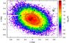 |
Fig. 1 Spatial Hess diagram of the RGB population of Fornax from a wide-field dataset (de Boer et al. 2011). The circles indicate the position of the GCs in the Fornax dSph, with positions according to Mackey & Gilmore (2003b). The solid ellipse indicates the core radius of the Fornax dSph. |
In this paper we use archival Hubble Space Telescope (HST) imaging presented in Buonanno et al. (1998, 1999) to determine the detailed SFH of each GC. We use a detailed synthetic CMD method to model the full CMD of each cluster while taking the photometric errors and completeness into account instead of fitting simple isochrones and ridgelines. This determines the accurate age and metallicity of each cluster and whether they are consistent with a single, short burst of star formation or if a more complex mix of stellar populations is present. As a byproduct of the SFH determination, we are then also able to determine the total stellar mass of each cluster, which can be compared to the total stellar mass of the Fornax dSph.
The paper is structured as follows: in Sect. 2 we outline the data reduction, followed by the sample selection and CMD construction in Sect. 3. Section 4 discusses the determination of the best-fit distance to each cluster, and in Sect. 5 we present the best-fit SFH results. Based on the quantitative SFH results, we derive the total stellar masses of the cluster in relation to the total mass of the Fornax field and present the results in Sect. 7. Finally, Sect. 8 discusses the results obtained from the SFH and the conclusions for the formation and evolution of the Fornax dSph.
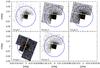 |
Fig. 2 Spatial distribution of stars within the HST pointings of each GC, with coordinates centred on the literature positions according to Mackey & Gilmore (2003b). Blue dashed lines indicate the tidal radius of each cluster, while the red solid circles for Fornax 3 and 4 indicate the region heavily affected by stellar crowding. For clusters 1, 2, 3, and 5 we limit our sample to the WFPC2 PC chip (smaller square coverage), while for Fornax 4 our sample consists of all stars within a radius of 48′′ (see Sect. 3). The representative foreground contamination region is constructed from stars outside the blue tidal radius region, except for Fornax 4, where a radius of 48″ is adopted. |
2. Data
To determine the detailed SFH of the GCs of the Fornax dSph, we used archival data. Deep images were obtained with HST/WFPC2 in the broadband F555W and F814W filters for each cluster, as discussed in detail in Buonanno et al. (1998, 1999). The data consist of several long exposures in each filter, accompanied by short exposures to include the otherwise saturated bright stars. For Fornax 1, 2, 3, and 5 the cluster centre was placed on the high-resolution PC chip, while the centre of Fornax 4 was located mainly on the WF3 chip.
All HST+WFPC2 images were downloaded from the Mikulski Archive for Space Telescopes (MAST1), and point spread function (PSF) fitting photometry was performed on them using hstphot (Dolphin 2000). hstphot is a stand-alone photometry package designed for use on WFPC2 data. In each instance, the associated data quality image from MAST was used to mask bad pixels in the image. Cosmic rays and hot pixels were identified and masked before multiple exposures taken with the same filter and pointing were combined. The offsets between the combined frames were then measured before hstphot was run simultaneously on all images.
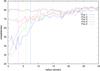 |
Fig. 3 Sampling completeness as a function of radius for each GC as derived from artificial star tests. Vertical lines indicate the radial cuts imposed on GCs 3, 4, and 5 to restrict the data sample to a completeness greater than ≈60 percent. |
A threshold of 3.5σ in a single frame was used to detect sources, while we required sources to be detected at an overall combined significance of 5σ across all images. The recommended parameters were used when running hstphot (i.e. refitting the sky background for all images using option 512), with the exception of those taken for Fornax 5, where a local sky background was measured. We also tested the effect of a weighted PSF fit, but found this did not noticeably improve the photometry in the crowded centres of the clusters (as gauged by the width of the main sequence on the resulting CMD).
To simulate observational conditions in the synthetic CMDs used to determine the SFH, we used artificial star test simulations. To this end, we carried out many simulations, in which a number of artificial stars (with known brightness) were placed on the observed images. These images were then analysed in exactly the same way as the original images, after which the artificial stars were recovered from the photometry. In this way, we obtained a look-up table that can be used to accurately model the effects of crowding and completeness as a function of magnitude (e.g. Stetson & Harris 1988; Gallart et al. 1996). The lookup-table was used in Talos to assign an individual artificial star (with similar colours and magnitudes) to each star in an ideal synthetic CMD and considering the manner in which this star is recovered to be representative of the effect of the observational biases.
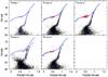 |
Fig. 4 Observed CMD diagrams of the five GCs in the Fornax dSph. Red datapoints show confirmed RR Lyrae stars collected from Mackey & Gilmore (2003a), Greco et al. (2007). Overlaid isochrones trace a metal-poor ([Fe/H] = −2.5 dex) population at a fixed age of 14 Gyr, taken from the Dartmouth Stellar Evolution Database isochrone set (Dotter et al. 2008). For each isochrone, we adopted a distance as derived from RR Lyrae stars assuming a metallicity as determined from spectroscopic measurements (see Table 1). |
3. Colour-magnitude diagrams
Figure 2 presents the spatial distribution of stars within each HST pointing, with coordinates centred on their literature positions according to Mackey & Gilmore (2003b). The literature tidal radius of each cluster is indicated by the blue circles, making it clear that the HST data does not sample the full stellar distribution of the clusters. Several clusters also suffer from extensive stellar crowding towards their centres, as shown in Fig. 3. The sampling completeness drops significantly for small radii in Fornax 3, 4, and 5, possibly impeding a full sampling of the CMD stellar populations in these clusters. Therefore, we excised the overcrowded central regions inside the radius indicated by the vertical lines in Fig. 3. To select a stellar sample for which the SFH was to be determined, we limited ourselves to the WFPC2 PC chip (smaller square footprint) for Fornax 1, 2, 3, and 5 to avoid introducing inhomogeneous data and to use the greater spatial resolution in the best way. Finally, we corrected the magnitude of each star for the effect of dust extinction using maps of Schlegel et al. (1998) to determine the extinction towards each individual star.
Figure 4 shows the resulting F814W and F555W-F814W CMD for each cluster, overlaid with isochrones from the Dartmouth Stellar Evolution Database isochrone set (Dotter et al. 2008) tracing metal-poor ([Fe/H] = −2.5 dex) populations at a fixed age of 14 Gyr. For each metallicity, we adopted a value of [α/Fe] consistent with the α-element distribution determined from high-resolution spectroscopic measurements (Letarte et al. 2006; Lemasle et al. 2014; Hendricks et al. 2016). Confirmed RR Lyrae stars for each cluster are indicated with red circles, according to data collected from Mackey & Gilmore (2003a), Greco et al. (2007).
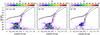 |
Fig. 5 Hess diagrams of Fornax 4 after correcting for MW and Fornax field background contamination, with different cuts for the cluster and background population, at 32′′, 48′′, and 64′′ (the tidal radius). A metal-poor ([Fe/H] = −2.5 dex, solid) and metal-rich ([Fe/H] = −1.5 dex, dashed) isochrone at a fixed age of 14 Gyr are overlaid to highlight the shape of population features. |
For each cluster, we also constructed Hess diagrams by computing the density of observed stars in small bins in the CMD. The Hess diagrams determined in this way contain stars of the Fornax GC and stars belonging to the MW and the Fornax dSph field population. To correct for these contaminants, we corrected the cluster CMDs by subtracting a representative comparison CMD for each sample. The comparison CMD Hess diagram was scaled using the spatial area subtended on the sky of each cluster and background sample (see Fig. 2) before subtraction. For the outer clusters, the coverage of our observations outside the tidal radius (blue circle in Fig. 2) is sufficient to sample the background contamination.
However, for Fornax 4 the observations cover very little area outside the literature tidal radius, providing a limited sampling of the background CMD features. As a result of the central location of Fornax 4, the surface density of contaminants is expected to dominate the density of cluster stars that are already well within the tidal radius. Therefore, contamination regions inside the tidal radius are still expected to provide a good background representation, while the larger area covered will lead to a better CMD sampling. To gauge this effect, we constructed a BG-contamination-corrected Hess diagram with three radial data cuts, at 32′′, 48′′, and 64′′ (the tidal radius), shown in Fig. 5. For the cut at the tidal radius, the Hess diagram shows stellar populations that are well traced by the overlaid isochrones, but a patchy CMD with strong residuals due to the limited sampling of CMD features in the background region. Conversely, for the innermost cut at half the tidal radius, only limited CMD features are present, indicating that the adopted background region samples and over-subtracts the cluster populations. Therefore, we adopted a radial cut at 48′′, in which case the Hess diagram recovers a well-defined stellar main-sequence turn-off and RGB while minimising the residual Fornax field populations.
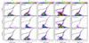 |
Fig. 6 Hess diagrams of the GCs in the Fornax dSph, showing the observed data adopted for each cluster (top row), the data in the MW and Fornax field background reference region (middle row, scaled to the same area as the observed data), and the difference between the two (bottom row). For the outer four clusters, the level of MW and Fornax field contamination within the cluster aperture is low. We therefore multiplied the reference Hess diagram for these clusters by a factor 10 to highlight features in the CMD. Overlaid (solid) isochrones trace a metal-poor ([Fe/H] = −2.5 dex) population at a fixed age of 14 Gyr, taken from the Dartmouth Stellar Evolution Database isochrone set (Dotter et al. 2008). We also show for Fornax 4 a more metal-rich ([Fe/H] = −1.5 dex) isochrone at a fixed age of 14 Gyr as the dashed line. For each isochrone, we adopted the distance given in Table 1 that was derived from RR Lyrae stars. |
Figure 6 shows the selected Hess diagrams for each cluster, displaying the observed data (top row), the MW, and Fornax field background reference region after scaling to the same area as the observed data (middle row) and the difference between the two (bottom row). Metal-poor ([Fe/H] = −2.5 dex) isochrones at a fixed age of 14 Gyr are overlaid as solid lines, while for Fornax 4 we also show a more metal-rich ([Fe/H] = −1.5 dex) isochrone (dashed line).
The CMDs for Fornax 1, 2, 3, and 5 displayed in Figs. 4 and 6 trace a well-defined stellar population locus consistent with a low metallicity and old age. Clusters Fornax 1 and 3 appear consistent with the [Fe/H] = −2.5 dex isochrone, while the RGB of Fornax 2 and 5 is redder than the isochrone, indicating a slightly higher metallicity (although still quite metal-poor). This is in line with results from unresolved metallicity-sensitive line indices (Larsen et al. 2012a). Clear signs of a blue HB are visible in Fornax 2, 3, and 5, indicating the presence of metal-poor stars. No clear HB population can be seen in Fornax 1, which might be due to the relatively low number of stars in this outer GC, leading to a sparsely populated RGB and HB. The four metal-poor GCs display colours at the main-sequence turn-off level in agreement with old ages, with metal-poor isochrones tracing the middle of the CMD distribution. The cluster sequences are well defined in the CMD, with little intrinsic dispersion and no clear signs of multiple composite populations.
Finally, the observed CMD of Fornax 4 shows a more complex mix of populations, with a range of populations at the main-sequence turn-off level and evidence for low levels of young stars (see Fig. 4). After subtracting the Hess diagram of the Fornax field star contamination (see Fig. 6), the CMD becomes more defined, with a clear main-sequence turn-off consistent with old ages. However, young populations are still visible in Fig. 6, which may be residual Fornax field populations due to imperfect background subtraction, given the high levels of contamination. When we consider only bright stars, Fornax 4 shows a well-defined thin red RGB, indicating more metal-rich and potentially younger stellar populations. No clear indication of a metal-poor RGB is seen in the CMD, suggesting that this cluster is different from the other four Fornax GCs.
4. Distance
A crucial parameter for determining the detailed SFH is the distance to each individual GC. An incorrect distance would lead to a systematic offset between the model and observed CMD, which leads to a bias in the stellar populations of the cluster by for instance adopting too young and too metal-poor populations in the case of a too large distance. The Fornax dSph is located at a distance of 147 ± 4 kpc ((m − M)V = 20.84 ± 0.04), determined using RR Lyrae stars, in good agreement with other measurements using the infrared tip of the RGB method and the horizontal branch (HB) level (Greco et al. 2005; Rizzi et al. 2007; Pietrzyński et al. 2009). The GCs of Fornax have also been the subject of variability studies, leading to the detection of RR Lyrae stars in each cluster, as plotted in Fig. 4 (Mackey & Gilmore 2003a; Greco et al. 2007).
However, the distance toward each cluster is not only dependent on the mean RR Lyrae brightness, but also on the metallicity of the cluster. The size of this effect can be significant, with a change in distance modulus of ≈0.2 mag when switching from a metallicity of [Fe/H] = −2.5 dex to [Fe/H] = −1.5 dex. This means that assuming an incorrect metallicity for the clusters would lead to a bias in the distance and consequently a bias in the SFH results.
To determine the distance toward each cluster, we used the spectroscopic metallicity studies conducted for each cluster. For Fornax 1, 2, and 3 we adopted metallicities from high-resolution spectroscopy of individual stars from Letarte et al. (2006), and for Fornax 4 and 5 we adopted the most recent integrated-light metallicity estimates from Larsen et al. (2012a). We then determined the intrinsic brightness of RR Lyrae stars of each metallicity using relations by Cacciari & Clementini (e.g. 2003), Clementini et al. (e.g. 2003), Gratton et al. (e.g. 2004). Following this, we compared the observed mean brightness of the RR Lyrae stars as presented in Mackey & Gilmore (2003a), Greco et al. (2007) and took the average visual dust extinction into account. This uniquely determines the distance towards each cluster. The adopted parameters for the Fornax GCs and their uncertainties are presented in Table 1. The table shows that all clusters are consistent within the uncertainties with a location inside the main body of Fornax. The outermost cluster Fornax 1 is located at a distance consistent with or slightly behind the Fornax centre, whereas the other four clusters are more consistent with being located slightly in front of the main body.
Adopted parameters for each globular cluster.
5. Star formation history
The SFH of each GC was determined using the SFH-fitting code Talos, described in detail in de Boer et al. (2012a). The SFH is derived on the basis of the extinction-free (F814W, F555W−F814W) CMD, corrected for foreground MW and Fornax field star contamination. A uniform bin size of 0.05 in colour and 0.1 in magnitude was used for all clusters except Fornax 4. For this cluster, we doubled the bin sizes because of the sparse sampling of CMD features after correcting for Fornax field contamination. No spectroscopic metallicity distribution function was used in the SFH determination because of the limited sample of spectroscopic observations available. We adopted the Dartmouth Stellar Evolution Database isochrone set (Dotter et al. 2008) in the SFH fitting, since this set was also used in the derivation of the SFH of the Fornax field population (de Boer et al. 2012b). For the SFH solution, metallicities were allowed to range from −2.5 ≤ [Fe/H] ≤ +0.3 dex with a spacing of 0.2 dex for ages between 0.5 and 14 Gyr with a spacing of 0.5 Gyr. While it is possible for a cluster to have a metallicity below [Fe/H] = −2.5 dex, isochrones which such low metallicities become degenerate, producing indistinguishable CMDs. Therefore, we only considered metallicities down to this limit.
The fitting procedure results in a 3D solution giving the star formation rate (SFR) for each age and metallicity, which is presented for each cluster in Fig. 7. By projecting this solution onto the age axis, we obtain the SFH, while projection onto the metallicity axis gives the chemical evolution history, presented in Fig. 8. To assess the width of SFR peaks in age and metallicity space, we fitted Gaussian profiles to the SFH to determine the mean position of the central peak and the variance. The Gaussian profiles are also shown as dashed lines in Fig. 8, with fitted values for age and metallicity presented in Table 2.
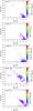 |
Fig. 7 Full 2D SFH solution derived for each of the five Fornax GCs from fits to the CMDs as shown in Fig. 6. Values for the SFR have been corrected for the missing mass fraction using values given in Table 1. |
Following the fitting procedure, Fig. 9 shows the observed and synthetic (F814W and F555W−F814W) CMD of each Fornax cluster and the residual in each bin in terms of Poissonian uncertainties. The residuals show that the synthetic CMDs are largely consistent with the observed CMDs within three sigma in each bin barring a small fraction of bins with positive residuals, indicating an overall good fit of the data. The synthetic CMDs correctly reproduce all evolutionary features in the lower CMD, including the location and spread of the main-sequence turn-off, subgiant branch, and the slope of the RGB.
Figures 7 and 8 show that Fornax 1, 2, 3, and 5 are all dominated by ancient metal-poor populations, consistent with the CMDs presented in Fig. 6, while Fornax 4 displays a peak at more intermediate age and metallicity. Each cluster displays a somewhat extended sequence in age-metallicity space caused by the ever-present age-metallicity degeneracy, which results in different combinations of age and metallicity producing a very similar CMD. This degeneracy is not fully broken when sampling the full CMD at high resolution, especially at old ages. Nonetheless, the combination of a well-sampled narrow main-sequence turn-off and a thin RGB places strong constraints on the possible age and metallicity of the cluster, as shown by the peaks in SFR. The SFH of each cluster also displays a small burst of star formation at young (2−4 Gyr) ages, which is due to the small numbers of blue straggler stars. These small peaks are ignored during the following discussion.
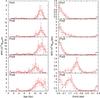 |
Fig. 8 SFH (left) and chemical evolution history (right) of the five GCs of the Fornax dSph as obtained from the HST F814W and F555W−F814W CMD. Values for the SFR have been corrected for the missing mass fraction using values given in Table 2. Dashed lines show the Gaussian profile that best fits the age and metallicity distribution, with parameters given in Table 2. |
The SFH of Fornax 1 peaks at an age of ≈12 Gyr, favouring an age slightly younger than the maximum allowed. The chemical evolution history peaks towards the lower limit in our parameter space, indicating that this is indeed a metal-poor ancient GC, consistent with a scenario in which it formed in a single short episode of star formation. The SFH of Fornax 3 is very similar, although the age distribution is broader and can be linked to the relatively wide RGB observed in Fig. 6. Likewise, Fornax 2 is also an ancient cluster with an age of ≈12 Gyr and a metallicity that peaks at the limit of our parameter space. This is slightly more metal-poor than the results from spectroscopic measurements, although broadly consistent within the uncertainties of the peak.
Fornax 5 peaks at a slightly younger age than the other metal-poor clusters, but shows a distribution in age wider than any of the other old clusters. This wide distribution might result in a younger average light-weighted age as observed by Strader et al. (2003). The chemical evolution history of Fornax 5 is wide, with a high SFR at −2.5 dex and a more defined Gaussian peak at [Fe/H] = −1.7 dex, consistent with measurements using unresolved metallicity indicators (Larsen et al. 2012a). Finally, the SFH of Fornax 4 displays many patchy low SFR populations, mosst likely a result of residual contamination by the underlying Fornax field, as seen in the CMD in Figs. 4 and 6. Nonetheless, the chemical evolution history shows a well-defined metallicity distribution peaking at [Fe/H] = −1.2 dex and a clear peak in the SFH at an age of ≈10 Gyr (see Table 2). These parameters are consistent with both the red RGB and relatively blue main-sequence turn-off in Fig. 5.
6. Testing for extended populations
After determining the detailed SFH of the Fornax GCs, we considered whether the clusters show any signs of composite multiple populations. An important consideration when judging the population spread in the clusters is the intrinsic uncertainty on age and metallicity that is due to the adopted SFH method. The ability to resolve an episode of star formation depends mainly on the photometric depth and associated photometric errors of the observed data. The method of determining the uncertainties of the solution also results in a smoothing of the SFH, which limits the resolution of the SFH. To determine the intrinsic resolution, we constructed a set of mock synthetic CMDs for single-burst populations, similar to the scheme proposed by Hidalgo et al. (e.g. 2011). The manner in which these single-burst populations are recovered will determine the intrinsic resolution of the SFH.
We constructed a synthetic CMD for each cluster, with an age and metallicity corresponding to the middle of the population bin in which the SFH peak is located, as shown in Fig. 8 and listed in Table 2. Subsequently, we convolved the CMD with artificial star test completeness results and photometric error curves from the observed CMD to simulate the observational conditions of each Fornax GC. The synthetic CMDs were subsequently analysed in exactly the same manner as the data, and the manner in which the single bursts are recovered indicates the intrinsic uncertainty due to the adopted method.
The recovered SFH for the synthetic bursts is shown in Fig. 10 for each cluster along with the SFH corresponding to a perfect recovery for comparison as the solid black histogram. The recovered SFH is fit by a Gaussian distribution, from which we determined the age of the central peak and the variance, as shown in Table 2.
Figure 10 shows that the central peak is correctly recovered for each cluster, barring small offsets towards younger ages for the most metal-poor clusters, which are most likely due to edge effects in the metallicity distribution. The Gaussian fits show that the widths of the distribution of recovered mock populations are similar to those of the cluster SFHs in Fig. 8. This means that we find no clear signs of extended populations in any of the clusters, given the smoothing induced by the data quality and SFH method. Age distributions in the recovered SFHs are slightly narrower than those in cluster SFHs, which might indicate that the clusters are more extended in age than delta function single-burst populations. However, the width of the distributions might also be affected by residual contamination, by blue straggler stars, and by unresolved binaries.
7. Total mass
With the results of the SFH, it is possible to derive the total mass formed in each GC directly from the CMD fitting. By integrating the SFR of each stellar population, we obtained the total mass in stars formed over the mass range 0.1−120 M⊙ under the assumption of a Kroupa initial mass function (IMF; Kroupa 2001). However, to obtain the full stellar mass of the GCs, we need to account for the fact that we did not sample the full stellar distribution of each cluster. To this end, we employed the stellar density models derived for the cluster by Mackey & Gilmore (2003b), where King profiles were fit to the stellar number counts as a function of radius.
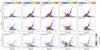 |
Fig. 9 Top: observed foreground-corrected Hess diagrams as used in the SFH determination for each cluster. Middle: best-fit model CMD obtained by Talos. Bottom: difference between the observed and best-fit CMD, expressed as a function of the uncertainty in each CMD bin. |
We used these best-fit models to compute the fraction of the stellar mass sampled by our target selection and SFHs. For each cluster, we constructed the 2D spatial distribution of stars according to the King profile parameters of Mackey & Gilmore (2003b). Subsequently, we convolved the distribution with the HST footprint and the radial cuts applied to remove spatial regions heavily influenced by stellar crowding. The observed and model distributions obtained in this way are shown in Fig. 11 for Fornax 4 to illustrate the process. We used the comparison between the total number of stars in each distribution to determine the fraction of stars and therefore mass missing from the SFH of each cluster, shown in Table 1. For the mass segregation with the Fornax clusters, the question remains whether the fits derived using relatively bright and massive stars provide a valid fit to the spatial distribution of stars of all masses. However, to probe this effect, better spatial resolution data extending down to the lower main sequence are needed.
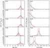 |
Fig. 10 Input and recovered SFH (left) and chemical evolution history (right) of mock stellar populations for each cluster based on the peaks of star formation in Fig. 8. The black solid histogram shows the input SFH, given the adopted binning of the solution. The red histograms show the recovered SFH, while the black dashed lines show the best-fit Gaussian distribution, with mean and variance listed in Table 2. |
Total mass in stars formed in each GC over the mass range 0.1−120 M⊙.
The resulting total mass derived for each GC after correcting for the missing mass fraction is shown in Table 3. The computed total stellar masses show that Fornax 3 is the most massive cluster in the Fornax dSph, followed by Fornax 5 and 2. As expected, the outermost cluster Fornax 1 has the lowest mass of the GC system, resulting in a sparsely populated CMD in Fig. 6. The computed masses agree reasonably well with the results of Mackey & Gilmore (2003b) given the error bars, and the order of cluster masses is also in line with unresolved absolute magnitudes (Larsen et al. 2012b).
Following the work of Larsen et al. (2012b), it is useful to compare the masses of the Fornax GCs to the total stellar mass in the Fornax dSph field. To compute the total stellar mass in Fornax, we used the data presented in de Boer et al. (2012b), where SFHs were determined within the same framework as the results presented here. Given the old age of stellar populations found in the outskirts of Fornax, we redetermined the SFH using the deep V, B − V data to gain the best possible sampling of the oldest main-sequence turn-off region. The SFH obtained in this way can be integrated to obtain the total stellar mass out to an elliptical radius of 0.8 degrees, which falls short of the tidal radius of 1.18 degrees (Irwin & Hatzidimitriou 1995). To obtain the total stellar mass out to the tidal radius, we corrected the stellar mass obtained from the SFH by assuming that the outer regions of Fornax display the same population mix and density as the outermost ellipse in de Boer et al. (2012b). The total stellar mass in the outermost region (as derived from the SFH) was scaled to the spatial area of the missing part and added to the derived SFH mass to obtain a total stellar mass within the tidal radius of (3.82 ± 0.12) × 107 M⊙. This value is lower than the results computed in de Boer et al. (2012b) as a result of the depth of the B−V data, leading to better constraints on the oldest populations that make up the bulk of the mass in Fornax.
The combined mass in the Fornax GCs is (9.57 ± 0.93) × 105 M⊙, which corresponds to 2.5 ± 0..2 percent of the total stellar mass in Fornax. However, the bulk of the stars in Fornax is metal-rich ([Fe/H] >− 1.5 dex), while the majority of the clusters are metal-poor. It is therefore useful to compare the total mass of the metal-poor clusters of (8.81 ± 0.92) × 105 M⊙ to the SFH-derived metal-poor ([Fe/H] <−2 dex) stellar mass in the Fornax main body of (44.9 ± 5.3) × 105 M⊙ to give a mass fraction of 19.6 ± 3.1 percent. This shows that the metal-poor globular clusters encompass a substantial fraction of the stellar mass of the Fornax dwarf galaxy. This recovered value for the total stellar mass of the cluster agrees with the results of Larsen et al. (2012b) when corrected for age effects.
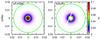 |
Fig. 11 Left: normalised spatial distribution for cluster Fornax 4 with a stellar density according to King profile fits from Mackey & Gilmore (2003b). The green (dashed) circle indicates the tidal radius. Right: spatial distribution for the cluster convolved with the actual coverage of the HST pointing, and the rejection of a central region due to incomplete data. Comparison between the two distributions allows us to determine the fraction of stars (and therefore mass) missing from the adopted sample. |
8. Discussions and conclusions
The SFH derived for the Fornax GCs shows that Fornax 1, 2, 3, and 5 are all old and metal-poor clusters, while Fornax 4 is dominated by more metal-rich and younger stars. The metallicities derived for the GCs (Fig. 8) agree with integrated-light and HR spectroscopic measurements (e.g. Letarte et al. 2006; Larsen et al. 2012a; Hendricks et al. 2016). However, the results obtained from the SFH fitting further quantify the age and metallicity distribution of the GCs and determine the mass in stars formed at each epoch.
The SFH of Fornax 1, 2, and 3 display a clear peak at [Fe/H] ≈−2.5 dex, with ages consistent with an ancient (≥10 Gyr) population. The results obtained from the CMD clearly confirm their status as some of the most metal-poor GCs known (Letarte et al. 2006). Results for Fornax 3 indicate that it is the most massive cluster in the Fornax dSph, with a mass more than twice that of any of the other clusters. The higher mass of Fornax 3 has not resulted in faster enrichment and a consequently higher metallicity. Instead, the SFH results agree well with the lower mass clusters Fornax 1 and 2.
The SFH of Fornax 4 is found to be different from that of the other clusters in Fornax, with a clear peak at an intermediate age of 10 Gyr and a metallicity of −1.2 dex. This shows that this cluster is substantially more metal-rich than the other clusters, in agreement with previous results based on integrated-light spectroscopy. Previous isochrone analysis of the age of Fornax 4 determined it to have an age ≈3 Gyr younger than the other Fornax GCs, which roughly agrees with the age peak in our SFH (Buonanno et al. 1999; Hendricks et al. 2016).
The location close to the centre of Fornax has given rise to multiple explanations on the nature of Fornax 4. In particular, Hardy (2002) and Strader et al. (2003) argued that it is the nucleus of the Fornax dSph, explaining its unusual populations, high metallicity, and central location. The spatial Hess diagram of Fornax in Fig. 1 shows that the position of Fornax 4 coincides with the highest density region of Fornax, which is also associated with the youngest populations of Fornax distributed in a shape inconsistent with that of the old populations (Battaglia et al. 2006). Our SFH shows that Fornax 4 is dominated by a single stellar population at an age of ≈10 Gyr with little dispersion in age and metallicity. However, there is residual star formation at other ages as a result of the high levels of Fornax field contamination. Nonetheless, the lack of ancient metal-poor populations argues against the nucleus scenario. This is consistent with the radial velocity of Fornax 4, which is distinctly different from that of the main body of Fornax (Larsen et al. 2012a; Hendricks et al. 2016). If this cluster is indeed a genuine globular cluster seen in projection to the centre of Fornax, it is still unclear why the cluster shows populations so different from others GCs in Fornax. A more complete photometric mapping of the inner regions of Fornax 4 with higher spatial resolution is needed to unambiguously separate the cluster population from the field contamination, preferably supported by spectroscopic observations of the bright cluster giants.
Finally, the CMD of Fornax 5 (see Fig. 6) shows a relatively red RGB that can be explained by a slightly higher metallicity and a wider age distribution than the other clusters, in line with light-weighted ages by Strader et al. (2003). We derived a relatively low mass with regard to integrated-light observations, which may be a result of the M/L ratio assumed for the cluster (e.g. Mackey & Gilmore 2003b). A younger age for the cluster would result in a smaller M/L ratio and a lower total stellar mass.
The total stellar masses of the Fornax GCs computed from the SFH is (9.57 ± 0.93) × 105 M⊙, which corresponds to a small fraction of the total stellar mass in the Fornax dSph. Comparison between the metal-poor clusters and the metal-poor field gives a mass fraction of 19.6 ± 3.1 percent, providing separate supporting evidence for the results of Larsen et al. (2012b). This unusually high mass fraction of the Fornax GCs compared to the field can be used to set valuable constraints on self-enrichment scenarios in which GCs were initially much more massive and lost most of their stars to the Fornax field (e.g. Schaerer & Charbonnel 2011; Bekki 2011; Larsen et al. 2012b). Clearly, unlocking the full formation history of the Fornax dSph and its individual components will provide vital insights into the complex formation scenario of the high end of the dwarf galaxy mass scale.
Acknowledgments
The research leading to these results has received funding from the European Research Council under the European Unions Seventh Framework Programme (FP/2007-2013) / ERC Grant Agreement No. 308024. This work was partly supported by the European Union FP7 programme through ERC grant number 320360. The authors would like to thank the anonymous referee for the comments that greatly helped us to improve the paper.
References
- Amorisco, N. C., & Evans, N. W. 2012, ApJ, 756, L2 [NASA ADS] [CrossRef] [Google Scholar]
- Bate, N. F., McMonigal, B., Lewis, G. F., et al. 2015, MNRAS, 453, 690 [NASA ADS] [CrossRef] [Google Scholar]
- Battaglia, G., Tolstoy, E., Helmi, A., et al. 2006, A&A, 459, 423 [NASA ADS] [CrossRef] [EDP Sciences] [Google Scholar]
- Battaglia, G., Irwin, M., Tolstoy, E., et al. 2008, MNRAS, 383, 183 [NASA ADS] [CrossRef] [MathSciNet] [Google Scholar]
- Bekki, K. 2011, MNRAS, 412, 2241 [NASA ADS] [CrossRef] [Google Scholar]
- Buonanno, R., Corsi, C. E., Fusi Pecci, F., Hardy, E., & Zinn, R. 1985, A&A, 152, 65 [NASA ADS] [Google Scholar]
- Buonanno, R., Corsi, C. E., Zinn, R., et al. 1998, ApJ, 501, L33 [NASA ADS] [CrossRef] [Google Scholar]
- Buonanno, R., Corsi, C. E., Castellani, M., et al. 1999, AJ, 118, 1671 [NASA ADS] [CrossRef] [Google Scholar]
- Cacciari, C., & Clementini, G. 2003, in Stellar Candles for the Extragalactic Distance Scale (Berlin: Springer Verlag), eds. D. Alloin, & W. Gieren, Lect. Notes Phys., 635, 105 [Google Scholar]
- Clementini, G., Gratton, R., Bragaglia, A., et al. 2003, AJ, 125, 1309 [NASA ADS] [CrossRef] [Google Scholar]
- Coleman, M. G., & de Jong, J. T. A. 2008, ApJ, 685, 933 [NASA ADS] [CrossRef] [Google Scholar]
- Coleman, M., Da Costa, G. S., Bland-Hawthorn, J., et al. 2004, AJ, 127, 832 [NASA ADS] [CrossRef] [Google Scholar]
- Coleman, M. G., Da Costa, G. S., Bland-Hawthorn, J., & Freeman, K. C. 2005, AJ, 129, 1443 [NASA ADS] [CrossRef] [Google Scholar]
- de Boer, T. J. L., Tolstoy, E., Saha, A., et al. 2011, A&A, 528, A119 [NASA ADS] [CrossRef] [EDP Sciences] [Google Scholar]
- de Boer, T. J. L., Tolstoy, E., Hill, V., et al. 2012a, A&A, 539, A103 [NASA ADS] [CrossRef] [EDP Sciences] [Google Scholar]
- de Boer, T. J. L., Tolstoy, E., Hill, V., et al. 2012b, A&A, 544, A73 [NASA ADS] [CrossRef] [EDP Sciences] [Google Scholar]
- de Boer, T. J. L., Tolstoy, E., Saha, A., & Olszewski, E. W. 2013, A&A, 551, A103 [NASA ADS] [CrossRef] [EDP Sciences] [Google Scholar]
- del Pino, A., Hidalgo, S. L., Aparicio, A., et al. 2013, MNRAS, 433, 1505 [NASA ADS] [CrossRef] [Google Scholar]
- Dolphin, A. E. 2000, PASP, 112, 1383 [NASA ADS] [CrossRef] [Google Scholar]
- Dotter, A., Chaboyer, B., Jevremović, D., et al. 2008, ApJS, 178, 89 [NASA ADS] [CrossRef] [Google Scholar]
- Dubath, P., Meylan, G., & Mayor, M. 1992, ApJ, 400, 510 [NASA ADS] [CrossRef] [Google Scholar]
- Gallart, C., Aparicio, A., & Vilchez, J. M. 1996, AJ, 112, 1928 [NASA ADS] [CrossRef] [EDP Sciences] [Google Scholar]
- Gallart, C., Aparicio, A., Zinn, R., et al. 2005, in IAU Colloq. 198: Near-fields cosmology with dwarf elliptical galaxies, eds. H. Jerjen, & B. Binggeli, 25 [Google Scholar]
- Gratton, R. G., Bragaglia, A., Clementini, G., et al. 2004, A&A, 421, 937 [NASA ADS] [CrossRef] [EDP Sciences] [Google Scholar]
- Greco, C., Clementini, G., Held, E. V., et al. 2005, ArXiv e-prints [arXiv:astro-ph/0507244] [Google Scholar]
- Greco, C., Clementini, G., Catelan, M., et al. 2007, ApJ, 670, 332 [NASA ADS] [CrossRef] [Google Scholar]
- Hardy, E. 2002, in Extragalactic Star Clusters, eds. D. P. Geisler, E. K. Grebel, & D. Minniti, IAU Symp., 207, 62 [Google Scholar]
- Hendricks, B., Boeche, C., Johnson, C. I., et al. 2016, A&A, 585, A86 [NASA ADS] [CrossRef] [EDP Sciences] [Google Scholar]
- Hidalgo, S. L., Aparicio, A., Skillman, E., et al. 2011, ApJ, 730, 14 [NASA ADS] [CrossRef] [Google Scholar]
- Hodge, P. W. 1961, AJ, 66, 83 [NASA ADS] [CrossRef] [Google Scholar]
- Irwin, M., & Hatzidimitriou, D. 1995, MNRAS, 277, 1354 [NASA ADS] [CrossRef] [Google Scholar]
- Kroupa, P. 2001, MNRAS, 322, 231 [NASA ADS] [CrossRef] [Google Scholar]
- Larsen, S. S., Brodie, J. P., & Strader, J. 2012a, A&A, 546, A53 [NASA ADS] [CrossRef] [EDP Sciences] [Google Scholar]
- Larsen, S. S., Strader, J., & Brodie, J. P. 2012b, A&A, 544, L14 [NASA ADS] [CrossRef] [EDP Sciences] [Google Scholar]
- Lemasle, B., de Boer, T. J. L., Hill, V., et al. 2014, A&A, 572, A88 [NASA ADS] [CrossRef] [EDP Sciences] [Google Scholar]
- Letarte, B., Hill, V., Jablonka, P., et al. 2006, A&A, 453, 547 [NASA ADS] [CrossRef] [EDP Sciences] [Google Scholar]
- Letarte, B., Hill, V., Tolstoy, E., et al. 2010, A&A, 523, A17 [NASA ADS] [CrossRef] [EDP Sciences] [Google Scholar]
- Mackey, A. D., & Gilmore, G. F. 2003a, MNRAS, 345, 747 [NASA ADS] [CrossRef] [Google Scholar]
- Mackey, A. D., & Gilmore, G. F. 2003b, MNRAS, 340, 175 [NASA ADS] [CrossRef] [Google Scholar]
- Nichols, M., Lin, D., & Bland-Hawthorn, J. 2012, ApJ, 748, 149 [NASA ADS] [CrossRef] [Google Scholar]
- Olszewski, E. W., Mateo, M., Harris, J., et al. 2006, AJ, 131, 912 [NASA ADS] [CrossRef] [Google Scholar]
- Pasetto, S., Grebel, E. K., Berczik, P., Chiosi, C., & Spurzem, R. 2011, A&A, 525, A99 [NASA ADS] [CrossRef] [EDP Sciences] [Google Scholar]
- Pietrzyński, G., Górski, M., Gieren, W., et al. 2009, AJ, 138, 459 [NASA ADS] [CrossRef] [Google Scholar]
- Pont, F., Zinn, R., Gallart, C., Hardy, E., & Winnick, R. 2004, AJ, 127, 840 [NASA ADS] [CrossRef] [Google Scholar]
- Rizzi, L., Held, E. V., Saviane, I., Tully, R. B., & Gullieuszik, M. 2007, MNRAS, 380, 1255 [NASA ADS] [CrossRef] [MathSciNet] [Google Scholar]
- Schaerer, D., & Charbonnel, C. 2011, MNRAS, 413, 2297 [NASA ADS] [CrossRef] [MathSciNet] [Google Scholar]
- Schlegel, D. J., Finkbeiner, D. P., & Davis, M. 1998, ApJ, 500, 525 [NASA ADS] [CrossRef] [Google Scholar]
- Shapley, H. 1938, Nature, 142, 715 [NASA ADS] [CrossRef] [Google Scholar]
- Stetson, P. B., & Harris, W. E. 1988, AJ, 96, 909 [NASA ADS] [CrossRef] [Google Scholar]
- Strader, J., Brodie, J. P., Forbes, D. A., Beasley, M. A., & Huchra, J. P. 2003, AJ, 125, 1291 [NASA ADS] [CrossRef] [Google Scholar]
- Tolstoy, E., Hill, V., & Tosi, M. 2009, ARA&A, 47, 371 [NASA ADS] [CrossRef] [Google Scholar]
- Yozin, C., & Bekki, K. 2012, ApJ, 756, L18 [NASA ADS] [CrossRef] [Google Scholar]
All Tables
All Figures
|
Fig. 1 Spatial Hess diagram of the RGB population of Fornax from a wide-field dataset (de Boer et al. 2011). The circles indicate the position of the GCs in the Fornax dSph, with positions according to Mackey & Gilmore (2003b). The solid ellipse indicates the core radius of the Fornax dSph. |
| In the text | |
|
Fig. 2 Spatial distribution of stars within the HST pointings of each GC, with coordinates centred on the literature positions according to Mackey & Gilmore (2003b). Blue dashed lines indicate the tidal radius of each cluster, while the red solid circles for Fornax 3 and 4 indicate the region heavily affected by stellar crowding. For clusters 1, 2, 3, and 5 we limit our sample to the WFPC2 PC chip (smaller square coverage), while for Fornax 4 our sample consists of all stars within a radius of 48′′ (see Sect. 3). The representative foreground contamination region is constructed from stars outside the blue tidal radius region, except for Fornax 4, where a radius of 48″ is adopted. |
| In the text | |
|
Fig. 3 Sampling completeness as a function of radius for each GC as derived from artificial star tests. Vertical lines indicate the radial cuts imposed on GCs 3, 4, and 5 to restrict the data sample to a completeness greater than ≈60 percent. |
| In the text | |
|
Fig. 4 Observed CMD diagrams of the five GCs in the Fornax dSph. Red datapoints show confirmed RR Lyrae stars collected from Mackey & Gilmore (2003a), Greco et al. (2007). Overlaid isochrones trace a metal-poor ([Fe/H] = −2.5 dex) population at a fixed age of 14 Gyr, taken from the Dartmouth Stellar Evolution Database isochrone set (Dotter et al. 2008). For each isochrone, we adopted a distance as derived from RR Lyrae stars assuming a metallicity as determined from spectroscopic measurements (see Table 1). |
| In the text | |
|
Fig. 5 Hess diagrams of Fornax 4 after correcting for MW and Fornax field background contamination, with different cuts for the cluster and background population, at 32′′, 48′′, and 64′′ (the tidal radius). A metal-poor ([Fe/H] = −2.5 dex, solid) and metal-rich ([Fe/H] = −1.5 dex, dashed) isochrone at a fixed age of 14 Gyr are overlaid to highlight the shape of population features. |
| In the text | |
|
Fig. 6 Hess diagrams of the GCs in the Fornax dSph, showing the observed data adopted for each cluster (top row), the data in the MW and Fornax field background reference region (middle row, scaled to the same area as the observed data), and the difference between the two (bottom row). For the outer four clusters, the level of MW and Fornax field contamination within the cluster aperture is low. We therefore multiplied the reference Hess diagram for these clusters by a factor 10 to highlight features in the CMD. Overlaid (solid) isochrones trace a metal-poor ([Fe/H] = −2.5 dex) population at a fixed age of 14 Gyr, taken from the Dartmouth Stellar Evolution Database isochrone set (Dotter et al. 2008). We also show for Fornax 4 a more metal-rich ([Fe/H] = −1.5 dex) isochrone at a fixed age of 14 Gyr as the dashed line. For each isochrone, we adopted the distance given in Table 1 that was derived from RR Lyrae stars. |
| In the text | |
|
Fig. 7 Full 2D SFH solution derived for each of the five Fornax GCs from fits to the CMDs as shown in Fig. 6. Values for the SFR have been corrected for the missing mass fraction using values given in Table 1. |
| In the text | |
|
Fig. 8 SFH (left) and chemical evolution history (right) of the five GCs of the Fornax dSph as obtained from the HST F814W and F555W−F814W CMD. Values for the SFR have been corrected for the missing mass fraction using values given in Table 2. Dashed lines show the Gaussian profile that best fits the age and metallicity distribution, with parameters given in Table 2. |
| In the text | |
|
Fig. 9 Top: observed foreground-corrected Hess diagrams as used in the SFH determination for each cluster. Middle: best-fit model CMD obtained by Talos. Bottom: difference between the observed and best-fit CMD, expressed as a function of the uncertainty in each CMD bin. |
| In the text | |
|
Fig. 10 Input and recovered SFH (left) and chemical evolution history (right) of mock stellar populations for each cluster based on the peaks of star formation in Fig. 8. The black solid histogram shows the input SFH, given the adopted binning of the solution. The red histograms show the recovered SFH, while the black dashed lines show the best-fit Gaussian distribution, with mean and variance listed in Table 2. |
| In the text | |
|
Fig. 11 Left: normalised spatial distribution for cluster Fornax 4 with a stellar density according to King profile fits from Mackey & Gilmore (2003b). The green (dashed) circle indicates the tidal radius. Right: spatial distribution for the cluster convolved with the actual coverage of the HST pointing, and the rejection of a central region due to incomplete data. Comparison between the two distributions allows us to determine the fraction of stars (and therefore mass) missing from the adopted sample. |
| In the text | |
Current usage metrics show cumulative count of Article Views (full-text article views including HTML views, PDF and ePub downloads, according to the available data) and Abstracts Views on Vision4Press platform.
Data correspond to usage on the plateform after 2015. The current usage metrics is available 48-96 hours after online publication and is updated daily on week days.
Initial download of the metrics may take a while.