| Issue |
A&A
Volume 590, June 2016
|
|
|---|---|---|
| Article Number | A34 | |
| Number of page(s) | 10 | |
| Section | Cosmology (including clusters of galaxies) | |
| DOI | https://doi.org/10.1051/0004-6361/201527540 | |
| Published online | 04 May 2016 | |
Model-independent characterisation of strong gravitational lenses
Universität Heidelberg, Zentrum für Astronomie,
Institut für Theoretische Astrophysik, Philosophenweg 12, 69120 Heidelberg, Germany
e-mail: This email address is being protected from spambots. You need JavaScript enabled to view it.
Received:
12
October
2015
Accepted:
4
December
2015
Abstract
We develop a new approach to extracting model-independent information from observations of strong gravitational lenses. The approach is based on the generic properties of images near the fold and cusp catastrophes in caustics and critical curves. The observables we used are the relative image positions, the magnification ratios and ellipticities of extended images, and time delays between images with temporally varying intensity. We show how these observables constrain derivatives and ratios of derivatives of the lensing potential near a critical curve. Based on these measured properties of the lensing potential, classes of parametric lens models can then easily be restricted to the parameter values that are compatible with the measurements, thus allowing fast scans of a large variety of models. Applying our approach to a representative galaxy (JVAS B1422+231) and a galaxy-cluster lens (MACS J1149.5+2223), we show which model-independent information can be extracted in each case and demonstrate that the parameters obtained by our approach for known parametric lens models agree well with those found by detailed model fitting.
Key words: dark matter / gravitational lensing: strong / methods: data analysis / methods: analytical / galaxies: clusters: general / galaxies: luminosity function, mass function
© ESO, 2016
1. Introduction and motivation
Fitting a parametric gravitational lens model to a given set of observed, gravitationally lensed images returns a set of parameter values that optimally reproduce the measured characteristics of the images with the given parametrised mass distribution. These kinds of models are generally not unique because the same set of images can usually be fitted by many different parametrisations. It is thus a question of conceptual and possibly practical importance as to what model-independent information is actually contained in strongly-lensed configurations of point-like or extended images. In fact, the only information we can infer on the deflector from the observables of strongly-lensed images is locally confined to the vicinity of these images. In this paper, we investigate which model-independent information can be obtained from a given set of gravitationally lensed images. As we show, this information amounts to ratios of derivatives of the lensing potential on or near the critical curve.
In Sect. 2, we derive which model-independent information about the gravitational lens can generally be obtained from the mutual distances, the ellipticities, and magnification ratios, as well as time delays of multiply-lensed images near fold and cusp points in critical curves. We further analyse the remaining degeneracies and estimate the measurement uncertainties and systematic errors of the results. In Sect. 3, we show how the parameters of parametrised mass models can be constrained by our approach. The permitted parameter ranges can then be compared to those obtained by direct model fitting. As representative example models, we consider axisymmetric and mildly elliptical models and investigate the influence of external shear on the ratios of derivatives. In Sect. 4, we then extract the model-independent information from the bright triple images in the galaxy lens JVAS B1422+231 and the cluster lens MACS J1149.5+2223. Specialising our approach to lens models from the literature, we compare model parameters inferred from our approach with parameter values obtained by detailed model fitting. We summarise our results in Sect. 5.
2. Model-independent characterisation of gravitational lenses near folds and cusps
According to Whitney (1955), the Fermat potential φ(x,y), x,y ∈ R2, of a sufficiently smooth gravitational lens model can be approximated around a singular point (x(0),y(0)) by the fourth-order polynomial 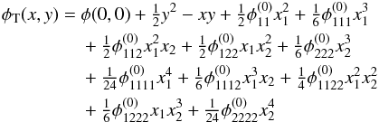 (1)if we introduce a coordinate system in the image plane with its origin shifted to (x(0),y(0)) and rotated such that
  (2)and a coordinate system in the source plane such that
  (3)without loss of generality. We further abbreviate
  (4)for i = 1,2.
Given φT(x,y), approximate lensing equations can be obtained from ∇xφT(x,y) = 0, where ∇x denotes the gradient with respect to x. These approximate lensing equations are then simplified by keeping only the leading-order terms in x, as explained in Schneider et al. (1992) or Petters et al. (2001).
2.1. Folds
At a fold singularity, coordinate systems can be chosen such that the conditions  (5)hold without loss of generality. In such coordinates, the approximate lensing equations to leading order in x read
 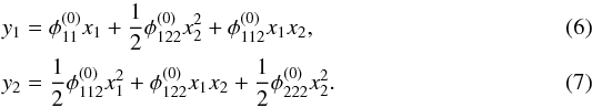 Evaluating these equations for both images of a source at y = (y1,y2), with image positions at xA and xB, a system of lensing equations can be set up and solved for the derivatives of φ at x(0) by eliminating y.
If available, we can use the observed ratios of the semi-major to the semi-minor axis of the images, 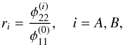 (8)to leading order in x and the equation for the time delay between the two images to obtain
 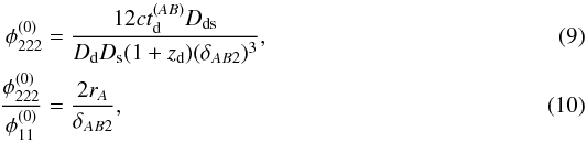 where c denotes the speed of light, zd the redshift of the lens plane,
  the measured time delay, Dds, Dd, and Ds the angular diameter distances between the lens and the source planes, the observer and the lens, and the observer and the source, respectively. δAB2 = xA2 − xB2 is the separation between (the centres of light of) the two images A and B at a fold in the lens plane. In the chosen coordinate system, the line connecting the two images is perpendicular to the critical curve, Schneider et al. (1992) (detailed derivations can be found in the Appendix).
The parity of the images can be determined by noting that the image leading in time has positive parity, while the following image has negative parity. Since the magnifications are equal for both images near a fold, no information can be gained to leading order from the magnification ratio.
For a physical interpretation of the ratios of derivatives of the lens potential, we rewrite Eq. (10) in terms of convergence, shear and flexion 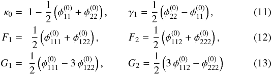 to obtain in the chosen coordinates
  (14)
(14)
2.2. Cusps
At a cusp singularity, we introduce coordinates such that  (15)as well as
  (16)and
  (17)hold. Again, this is possible without loss of generality, Schneider et al. (1992). Figure 1 shows the coordinate systems in the source and image planes for this cusp case.
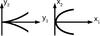 |
Fig. 1 Cusp singular point at the origins of the coordinate systems in the source and image planes defined by Eqs. (15)−(17). |
We label the three images such that image A is closest to the cusp inside the critical curve and has negative parity, while B and C have positive parity and fall above and below the critical curve, respectively. The image coordinates then satisfy  The configuration with opposite parities can be calculated analogously. The observed image configuration is degenerate with respect to the parity of their images until time delay information is included to decide which of the images is leading in time and thus has positive parity. This implies that
  and
and  are only determined up to their signs without time delay information. Hence, we choose
  and
and  to fix the signs in the lensing equations.
As a result, the Taylor-expanded lensing equations to leading order in x read  Using the same notation for the constants and observables as for the folds, we find
  these expressions are derived in the Appendix.
If the images are extended and time delays are available, Eqs. (23) and (25) can be combined to determine  . As the coordinate differences δijk, i,j = A,B,C, k = 1,2 between the images are not observable, we express them in terms of the measurable angles enclosed by the lines connecting A, B, and C,
  with αi, i = A,B,C, denoting the angles at the vertices i of the image triangle.
Even if magnification ratios are prone to large uncertainties, we consider using them, as they allow us to determine the absolute position of one image. Inserting the image position into the lensing equations Eqs. (21) and (22), the source position can be determined. The latter, in turn, can be used to estimate the effect of truncating the Taylor approximation (as further detailed in Sect. 2.3) or to calculate the image positions assuming a certain lens model. This allows us to test whether a given model describes an observed image configuration, or to predict positions of further images not located in the vicinity of the critical curve.
Without loss of generality, we determine xA, starting from the system of equations for the observable magnification ratios μAB and μAC,  where the ratios
  and
and  are given by the right-hand sides of Eqs. (24) and (25), respectively. Using the coordinate distances δijk from Eqs. (26) to (28) to replace xBi and xCi, i = 1,2, we can solve for xA and obtain
  Table 1 summarises the model-independent information that can be determined for the different combinations of given observables.
Model-independent information that can be determined for different combinations of observables at folds and cusps.
2.3. Uncertainties, errors and degeneracies
Each (ratio of) potential derivatives in Sect. 2 is subject to measurement uncertainties, a possible systematic error from signal processing, and a systematic deviation from the true value due to truncating the Taylor approximation after the leading order.
Statistical and systematic uncertainties can be propagated as usual, if given. Otherwise, calculating the results for all possible combinations of observables yields a range of values whose width indicates their uncertainties, because we expect the results to be independent of the specific image pair they are derived from. For example, by Eq. (10),  can be calculated from the axis ratios of both images A and B. The difference between the two results is an estimate for the combined observational and methodical uncertainties. For potential ratios at a cusp, the number of possible ways to derive the same quantity is increased by the third image, thus improving the uncertainty estimate.
The possible bias due to truncating the Taylor series of the potential is expected to decrease the closer the images are to the critical curve and the closer the source is to the caustic. At a cusp, these distances can be calculated as described in Sect. 2.2, if the required observables are available.
Since the accuracy of the Taylor approximation is model-dependent, a specific lensing potential needs to be assumed to estimate it. For elliptical models (elliptical potentials or surface-mass densities with singular isothermal density profiles, as detailed in the Appendix) of moderate ellipticity ≲0.2, we obtain deviations of a few percent for sources closer to the caustic than ~5% of the maximum extent of the caustic. In this case, results from time delays deviate by ~0.1% and ratios of potential derivatives by up to 3.5%. The lower accuracy of the latter is due to the Taylor-expanded lensing equations having been further linearised, which is not necessary for the time-delay equation (details about the calculations can be found in the Appendix). Our estimates for the accuracy of results from time delays agree with similar estimates by Congdon et al. (2008).
Furthermore, the possible bias due to the restriction to leading-order terms is negligible for axisymmetric and elliptical models because their symmetry implies that most of the omitted terms vanish.
As already pointed out by Gorenstein et al. (1988) and further developed by Schneider & Sluse (2014), several continuous transformations can be applied to the lens-modelling equations, leaving the observables invariant. Therefore, we still have the freedom to scale all derivatives of φ by a factor λ ∈R. This would only change the source position, which is not observable. The ratios of the derivatives remain invariant, and only the time delay can be used to break the degeneracy.
3. Model selection
While our approach to extracting model-independent information on strong gravitational lenses from the observables is new to our knowledge, numerous ways to constrain parameters for lens models have been developed in the past, e.g. Bartelmann (1996), Gorenstein et al. (1988), Grossman & Narayan (1988), Hammer (1992), Jullo et al. (2007), Keeton (2001), Limousin et al. (2005), Narayan (1986), Narayan & Grossman (1989), Oguri (2010), and Suyu (2012). To connect our work to previous studies, we now relate our model-independent (ratios of) potential derivatives to those of specific lens models to constrain their parameters.
For any gravitational lens producing one image pair at a fold singularity only, we can determine a single model parameter by means of Eq. (10), and use Eq. (9) to break the scaling degeneracy discussed in Sect. 2.3. At a cusp singularity with three neighbouring images, we have Eqs. (24) and (25) to determine up to two model parameters and break the scaling degeneracy with Eq. (23).
If the number of parameters exceeds the number of equations, the system of equations is underdetermined and a family of model parameters that satisfies the observational constraints is obtained as a solution set, unless the system is inconsistent owing to contradictory observations, or further information about the lens is available from non-lensing measurements, e.g. from observed velocity dispersions along the line of sight. Multiple sets of images from different sources at several singular points allow us to further narrow the range of feasible model parameters.
3.1. Axisymmetric lens models
As cusps in axisymmetric models always degenerate to a point singularity in the source plane, next to which sources form two images on opposite sides of the lens, the only applicable axisymmetric case for our approach are double images at radial critical curves. Hence, models with tangential critical curves only, such as the point mass or the singular isothermal sphere, can be excluded from the analysis. Furthermore, lying much closer to the lens centre than the tangential critical curves, images near radial critical curves are hard to detect and, so far, only a few of them have been found; see Molikawa & Hattori (2001) and Meneghetti et al. (2013) for an overview of the current observational status. Despite the restricted number of viable axisymmetric models, such as the non-singular isothermal sphere, the Plummer (1911), Navarro-Frenk-White (Navarro et al. 1997), and Hernquist (1990) models and the small number of confirmed, observed radial arcs, this class of model may still prove useful for primary lens models when adding external shear, as detailed in Sect. 3.3.
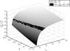 |
Fig. 2 Dependence of |
Moreover, to show how model parameters can be obtained in the case of an underdetermined system of equations, we consider the subclass of non-singular axisymmetric models given by 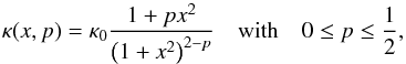 (33)as defined in Schneider et al. (1992). For p = 0, the distribution yields the Plummer model, for p = 1 / 2, we obtain a non-singular isothermal sphere. In these two cases, κ0 is given by
 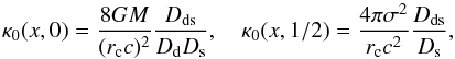 (34)where G denotes the gravitational constant, M the total lensing mass, rc the finite core radius of the lens, and σ2 the (measurable) velocity dispersion along the line of sight. The other quantities remain the same as defined in Sect. 2.1.
As x(0) is only determined numerically for given values of p and κ0, we obtain the ratio of derivatives dependent on p and κ0 as shown in Fig. 2 in the parameter range of p ∈ [0,1 / 2] and κ0 ∈ (1,10]. Given measured values for , the viable (p,κ0)-sets can be read off the graph, as indicated by the black area for the example range of  .
.
3.2. Elliptical lens models
Elliptical lens models can be further divided into two classes, elliptical mass distributions and elliptical lensing potentials, as compared in Kassiola & Kovner (1993). For large ellipticities, the latter generate dumb-bell shaped, unrealistic mass distributions, while for small ellipticities an equivalence relation to elliptical mass distributions can be found (see Sect. 5 of Kassiola & Kovner 1993, for details), such that elliptical potentials yield similar observables as elliptical mass distributions. To simplify calculations further, an axi-symmetric primary potential with external shear can also be considered equivalent in many cases of small ellipticities, as stated in Kovner (1987).
For the general case of arbitrary ellipticity, we now calculate the model parameters of a singular isothermal ellipse (SIE) as a representative example model of elliptical mass distributions, which we test for its suitability to describe the gravitational lensing configurations shown in Sect. 4. The deflection potential of an SIE in polar coordinates is given by  (35)with
 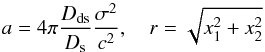 (36)and
  (37)where f denotes the axis ratio of the semi-minor to the semi-major axis in addition to the quantities already introduced.
Inserting ψ into the lensing potential φ(x) = 1 / 2(x − y)2 − ψ(x) and calculating the derivatives of this lens model as required by Eqs. (24) and (25), we can use these equations to solve for a and f to obtain  (38)for images in the vicinity of a cusp singularity on the semi-major axis of the lens and
  (39)for images in the vicinity of a cusp singularity on the semi-minor axis of the lens, with given by the right-hand side of Eq. (24) and by the right-hand side of Eq. (25) containing the measured quantities.
Measured quantities for B1422+231 as summarised in JVAS Collaboration (1992).
3.3. External shear
External shear is included into the analysis by adding the term  (40)to the lensing potential φ(x) of the primary gravitational lens, where Γi, i = 1,2 are real constants. They parametrise the external shear whose orientation θ and magnitude Γ are given by
  (41)Since φΓ is quadratic in the coordinates, second-order derivatives of the lensing potential change to
  and all higher-order derivatives remain unchanged. Thus, information from measured time delays is also not affected. This implies that external shear only affects the denominator of the ratios of derivatives in Eqs. (10), (24), and (25). For a fixed, measured right-hand side, the convergence of the primary model with external shear changes compared to the convergence of a model without external shear κ(x(0)) according to
 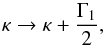 (45)now to be taken at the new position of the critical curve after introducing the external shear.
Since adding a constant external shear is a global property of the lens mapping, a consistency check can be established by comparing the values of Γi, = 1,2 determined by several sets of images. For this, the shear values obtained at different singular points have to be aligned by rotation into one global coordinate system.
4. Examples
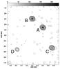 |
Fig. 3 MERLIN map of B1422+231 at 5 GHz radio frequency, shown here to define our labelling of the four gravitationally lensed images. Images A, B, and C are close to a cusp singularity, A being closest to the singular point. Image D is on the opposite side and thus not included in our data analysis. |
4.1. Galaxy lensing – JVAS B1422+231
JVAS B1422+231, as first described in Patnaik et al. (1992), is a quadruple-image gravitational lens at z = 0.34 showing three images of a source at z = 3.62 lying close together, as shown in Fig. 3. The measured data for this system is summarised in Table 2. They suggest that the images A, B, and C originate from a source near a cusp singularity in the caustic. Following our earlier notation, we label the images as shown in Fig. 31.
Since the time delays in Table 2 imply that image A follows both B and C, we conclude that A must have negative parity, while B and C must have positive parity (see also Congdon et al. 2008). Applying Eqs. (23)−(25) to the data in Table 2, we obtain the model-independent information after all observed image positions have been converted to radians 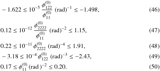 Using Eq. (38) on these ratios, we infer the model parameters of an SIE
  (51)which, solving a for σ, yields a velocity dispersion of
  (52)
(52)
These parameter values agree well with those found by Bradač et al. (2002) and Kormann et al. (1994): Kormann et al. (1994) determine the velocity dispersion of B1422+231 to be around 200 km s-1 for axis ratios between 0.35 and 0.60, while Bradač et al. (2002) get an axis ratio of 0.68 with an SIE that includes external shear and velocity dispersions of 190 km s-1. Although being consistent with each other and our results, both methods yield χ2 values per degree of freedom much larger than unity, rejecting the hypothesis that the resulting model parameters are (locally) optimal.
To assess the quality of our Taylor approximation in this case, we can determine the source position as described in Sect. 2.2 to obtain  (53)Furthermore, taking into account that the Einstein radius of the lens is of the order of 1′′, as estimated by the distance between the images A and D, a distance of the source to the singular point of the order of 10 mas implies that the Taylor-expanded ratios of derivatives should deviate only by a few percent from their true value, as argued in Sect. 2.3.
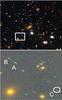 |
Fig. 4 Multi-wavelength image of the galaxy cluster MACS J1149.5+223, taken by the Hubble space telescope (top). The white box marks the position of the three gravitationally lensed images. A, B, and C (bottom) used for the mass reconstruction within the galaxy cluster. Image credits: NASA, ESA, and M. Postman (STScI), and the CLASH collaboration. |
4.2. Galaxy cluster lensing – MACS J1149.5+2223
The galaxy cluster MACS J1149.5+223, where a multiply-imaged supernova was recently detected (Kelly et al. 2014) is an X-ray bright, strongly lensing cluster at redshift z = 0.544, as described in Ebeling et al. (2007). For the three images of a source at z = 1.89 in the right part of Fig. 4, the CLASH collaboration has determined the distances between the images  (54)with the image ellipticities and their rms-errors obtained from SExtractor
  (55)Using the distances of Eq. (54) in radians and the image ellipticities of Eq. (55), we obtain
  Lacking time-delay information, we can neither determine the parity of the images nor gain further information as to whether the images are in the vicinity of the cusp on the semi-minor or semi-major axis of the lens. From the observed values, the model parameters for a singularity on the semi-major axis of an SIE are
  (58)and if the images are in the vicinity of a cusp singularity at the semi-minor axis of an SIE,
  (59)From these parameters the velocity dispersion for both cases, Eqs. (58) and (59), is derived to be
  (60)which agrees well with the measured values that fall between 500 and 1270 km s-1 from Smith et al. (2009).
Because of the different definitions and the addition of further visible mass content to the halo of dark matter, there is a large, but consistent range of mass estimates obtained for MACS J1149 of the order 1015 M⊙ (Limousin et al. 2005; Smith et al. 2009; Umetsu et al. 2014; Zitrin et al. 2015), which agrees with the estimated mass of an SIE, given the observables for MACS J1149 ![Mathematical equation: \begin{eqnarray} M_{200} = \dfrac{\pi\sigma^2}{200G}\, D_\mathrm{d} \in \left[6.56, 9.46 \right]\,10^{15}\,M_{\odot} , \label{eq:mass_SIE} \end{eqnarray}](/articles/aa/full_html/2016/06/aa27540-15/aa27540-15-eq174.png) (61)where M200 is the dark halo mass at r200, the radius enclosing a mean overdensity of 200 times the critical density of the universe. Calculating the dark matter mass enclosed within the critical curve, we arrive at
(61)where M200 is the dark halo mass at r200, the radius enclosing a mean overdensity of 200 times the critical density of the universe. Calculating the dark matter mass enclosed within the critical curve, we arrive at ![Mathematical equation: \begin{eqnarray} M_{\mathrm{cc}} = \dfrac{4 \pi^2 \sigma^4}{G c^2}\, \dfrac{D_\mathrm{d} D_\mathrm{ds}}{D_\mathrm{s}} \in \left[1.49, 3.09 \right]\,10^{14}\,M_{\odot} . \end{eqnarray}](/articles/aa/full_html/2016/06/aa27540-15/aa27540-15-eq177.png) (62)Comparing this value to the total mass (including luminous matter) found by Zitrin et al. (2015), Mcc = 9.83 × 10¹³ M⊙, we observe that the numbers are close. A more detailed comparison cannot be performed yet, since we do not include luminous matter in our model and only derive our mass estimate from a single set of three images close to a critical curve.
(62)Comparing this value to the total mass (including luminous matter) found by Zitrin et al. (2015), Mcc = 9.83 × 10¹³ M⊙, we observe that the numbers are close. A more detailed comparison cannot be performed yet, since we do not include luminous matter in our model and only derive our mass estimate from a single set of three images close to a critical curve.
5. Summary and discussion
We have studied which model-independent characteristics of strong gravitational lenses can be extracted directly from observational data. These observational data include the distances, ellipticities, magnification ratios, and time delays of multiply gravitationally-lensed images of sources close to fold and cusp singularities. Taylor-expanding the lensing potential around these singular points and choosing a special coordinate system, we set up a system of non-linear, approximate lensing equations. We solved these equations for the derivatives of the lensing potential at the cusps and folds. As the system is underdetermined even in the leading-order approximation, we could not determine the derivatives directly, but rather obtained ratios of derivatives. These are connected to physically more intuitive quantities like ratios of flexion and convergence. Time-delay information was used to determine the parities of the images. With given magnification ratios, the source position can be reconstructed, which allows us to estimate the accuracy of the Taylor expansion of the lensing potential. Furthermore, assuming a specific lens model, we showed that the derivatives of this lens model can be used to determine lens-model parameters. The application of our method to the galaxy-lensing configuration of JVAS B1422+231 and the galaxy-cluster lensing configuration of MACS J1149.5+2223 demonstrated that the model-independent information is capable of reproducing parameter values for an SIE that agree well with measured values and those obtained by χ2-parameter-estimation. Next, we plan to study more realistic potentials with substructure perturbations. It remains to be tested how generic our approach is in practice, i.e. to what subsample of gravitational-lens systems it can safely be applied.
Note that common labelling interchanges A and B in Fig. 3.
Acknowledgments
We wish to thank Mauricio Carrasco, Dan Coe, Matteo Maturi, Massimo Meneghetti, Sven Meyer, Eberhard Schmitt, Gregor Seidel, Keiichi Umetsu, Gerd Wagner, and Leonard Wirsching for helpful discussions. We gratefully acknowledge the support by the Deutsche Forschungsgemeinschaft (DFG) WA3547/1-1.
References
- Bartelmann, M. 1996, A&A, 313, 697 [NASA ADS] [Google Scholar]
- Bradač, M., Schneider, P., Steinmetz, M., et al. 2002, A&A, 388, 373 [NASA ADS] [CrossRef] [EDP Sciences] [Google Scholar]
- Congdon, A. B., Keeton, C. R., & Nordgren, C. E. 2008, MNRAS, 389, 398 [NASA ADS] [CrossRef] [Google Scholar]
- Ebeling, H., Barrett, E., Donovan, D., et al. 2007, ApJ, 661, L33 [NASA ADS] [CrossRef] [Google Scholar]
- Gorenstein, M. V., Shapiro, I. I., & Falco, E. E. 1988, ApJ, 327, 693 [NASA ADS] [CrossRef] [Google Scholar]
- Grossman, S. A., & Narayan, R. 1988, ApJ, 324, L37 [NASA ADS] [CrossRef] [Google Scholar]
- Hammer, F. 1992, in Distribution of Matter in the Universe, eds. G. A. Mamon, & D. Gerbal, 81 [Google Scholar]
- Hernquist, L. 1990, ApJ, 356, 359 [NASA ADS] [CrossRef] [Google Scholar]
- Jullo, E., Kneib, J.-P., Limousin, M., et al. 2007, New J. Phys., 9, 447 [Google Scholar]
- JVAS Collaboration 1992, Jodrell/VLA Astrometric Survey (JVAS), http://www.jb.man.ac.uk/research/gravlens/lensarch/B1422+231/B1422+231.html [Google Scholar]
- Kassiola, A., & Kovner, I. 1993, ApJ, 417, 450 [NASA ADS] [CrossRef] [Google Scholar]
- Keeton, C. R. 2001, ArXiv e-prints [arXiv:astro-ph/0102340] [Google Scholar]
- Kelly, P. L., Rodney, S. A., Treu, T., et al. 2014, ATel, 6729, 1 [NASA ADS] [Google Scholar]
- Kormann, R., Schneider, P., & Bartelmann, M. 1994, A&A, 286, 357 [NASA ADS] [Google Scholar]
- Kovner, I. 1987, ApJ, 312, 22 [NASA ADS] [CrossRef] [Google Scholar]
- Limousin, M., Kneib, J.-P., & Natarajan, P. 2005, MNRAS, 356, 309 [NASA ADS] [CrossRef] [Google Scholar]
- Meneghetti, M., Bartelmann, M., Dahle, H., & Limousin, M. 2013, Space Sci. Rev., 177, 31 [NASA ADS] [CrossRef] [Google Scholar]
- Molikawa, K., & Hattori, M. 2001, ApJ, 559, 544 [NASA ADS] [CrossRef] [Google Scholar]
- Narayan, R. 1986, in Quasars, eds. G. Swarup, & V. K. Kapahi, IAU Symp., 119, 529 [Google Scholar]
- Narayan, R., & Grossman, S. 1989, in Gravitational Lenses in Honor of Bernard F. Burke’s 60th Birthday, eds. J. N. Hewitt, J. M. Moran, B. F. Burke, & K. Y. Lo, 31 [Google Scholar]
- Navarro, J. F., Frenk, C. S., & White, S. D. M. 1997, ApJ, 490, 493 [NASA ADS] [CrossRef] [Google Scholar]
- Oguri, M. 2010, PASJ, 62, 1017 [NASA ADS] [Google Scholar]
- Patnaik, A. R., Browne, I. W. A., Walsh, D., Chaffee, F. H., & Foltz, C. B. 1992, MNRAS, 259, 1P [NASA ADS] [CrossRef] [Google Scholar]
- Petters, A. O., Levine, H., & Wambsganss, J. 2001, Singularity Theory and Gravitational Lensing, Progress in Mathematical Physics, Vol. 21 (Birkhäuser) [Google Scholar]
- Plummer, H. C. 1911, MNRAS, 71, 460 [CrossRef] [Google Scholar]
- Schneider, P., & Sluse, D. 2014, A&A, 564, A103 [NASA ADS] [CrossRef] [EDP Sciences] [Google Scholar]
- Schneider, P., Ehlers, J., & Falco, E. E. 1992, Gravitational Lenses, Astronomy and Astrophysics Library (New York: Springer) [Google Scholar]
- Smith, G. P., Ebeling, H., Limousin, M., et al. 2009, ApJ, 707, L163 [NASA ADS] [CrossRef] [Google Scholar]
- Suyu, S. H. 2012, MNRAS, 426, 868 [NASA ADS] [CrossRef] [Google Scholar]
- Umetsu, K., Medezinski, E., Nonino, M., et al. 2014, ApJ, 795, 163 [NASA ADS] [CrossRef] [Google Scholar]
- Whitney, H. 1955, The Annals of Mathematics, 62, 374 [CrossRef] [Google Scholar]
- Zitrin, A., Fabris, A., Merten, J., et al. 2015, ApJ, 801, 44 [NASA ADS] [CrossRef] [Google Scholar]
Appendix A: Derivations
Appendix A.1: Folds
The Taylor expansions of the derivatives at the centre of light image points i = A,B are given by 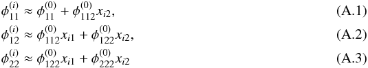 from which follows
 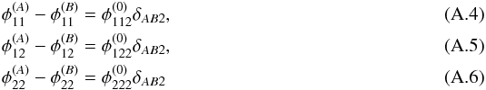 from which can be deduced
 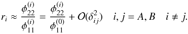 (A.7)Inserting the Taylor expansions into the lensing equations, Eqs. (6) and (7), we obtain
 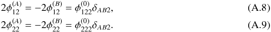 From Eq. (A.8) we cannot retrieve any information about the ratio of the derivatives, as the equation is also solved by setting
  . Using
  in Eq. (A.9), we arrive at
  (A.10)
Appendix A.2: Cusps
Subtracting the first lensing equation, Eq. (21) for B and C from A, respectively, Eq. (24) can be immediately obtained. Subsequently, the second lensing equations, Eq. (22), for the three images are analogously subtracted and the two resulting equations linearised. The Taylor expansions of the second order derivatives of image i,j = A,B,C with i ≠ j are 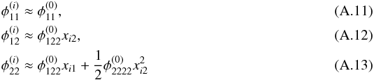 from which follows
 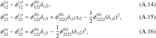 where we used
  in the last step. Applying these relations to the two resulting, linearised lensing equations yields
  (A.17)To be able to set up this equation, we require that xA2 ≠ 0. This is a reasonable requirement, if the images are not supposed to lie at the singular point. Assuming that δAB has an angle α with the x1-axis of the coordinate system, all coordinate distances δijk can be expressed in terms of δij, the observed angles αi, i = A,B,C, and α:
  so that we can solve Eq. (A.17) for α
 (A.22)Subtracting the ratios of two images, i = A,B,C
 (A.23)and inserting Eq. (24), we obtain Eq. (25).
Analogously to the fold case derived in Schneider et al. (1992), we can derive the time delay to leading order for the cusp between two of the three images i and j, with i,j = A,B,C, i ≠ j
Appendix B: Deviations due to the Taylor approximation
For the fold in the leading order approximation, Eq. (9) implies the deviations due to the Taylor approximation  (B.1)given an analytical lens model from which the image positions and potential derivatives are determined for a predefined source position with a certain distance dy to the fold singularity in the source plane.
For the cusp, we analogously obtain the following estimates for Eqs. (23) and (24) with i = B,C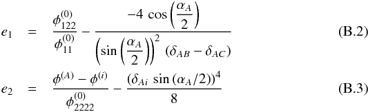 and similar expressions for the remaining images B and C.
Inserting a potential to calculate the Taylor errors for a specific case, we use a singular isothermal potential (SIEP) with the deflection potential  (B.4)in which f denotes the axis ratio, and the deflection potential of a singular isothermal ellipse (SIE) in polar coordinates given by
  (B.5)with
  (B.6)We consider the representative models with parameters a = 1 and f = 0.95,0.9,0.8 for both model types. To investigate the influence of the distance to the singularity, we generate four different point-source positions and determine their respective image positions with respect to the singularity in the image plane from the analytic models. Given the distance of the singular point to the origin dy = ||y(0)|| in the source plane before the transformation to the coordinate system in which y(0) = (0,0), the four different sources are located at distances 0.01,0.1,1,2,5% dy on the line that connects the singular point with the origin in the source plane in the case of the fold. To avoid xA2 = 0 in the cusp case, we arbitrarily choose to put the sources on a line that crosses the singularity with slope m = tan(α) = π × 10-4.
Calculating the errors of the leading order Taylor approximation to the ratios of derivatives of the analytic potentials as defined in Eq. (B.1), we arrive at the results shown in Fig. B.1, choosing the fold point in the source plane that is farthest away from the cusps on the coordinate axes. Figure B.2 shows analogous results for the cusp located on the y1-axis for the errors defined in Eqs. (B.2) and (B.3). For the latter, we inserted i = B.
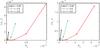 |
Fig. B.1 Dependence of the errors due to leading-order Taylor approximation of the potential ratios on the distance to the fold singularity as defined in Eq. (B.1) for the representative examples of an SIE (left) and an SIEP (right) for the parameter values a = 1 and f = 0.95 (black solid line), f = 0.9 (green dashed line), and f = 0.8 (red dash-dotted line). |
 |
Fig. B.2 Dependence of the errors due to leading-order Taylor approximation of the potential ratios on the distance to the cusp singularity, as defined in Eqs. (B.2) (top) and (B.3) (bottom) for the representative examples of an SIE (left) and an SIEP (right) for the parameter values a = 1 and f = 0.95 (black, solid line), f = 0.9 (green, dashed line), and f = 0.8 (red, dash-dotted line). |
All Tables
Model-independent information that can be determined for different combinations of observables at folds and cusps.
All Figures
|
Fig. 1 Cusp singular point at the origins of the coordinate systems in the source and image planes defined by Eqs. (15)−(17). |
| In the text | |
|
Fig. 2 Dependence of |
| In the text | |
|
Fig. 3 MERLIN map of B1422+231 at 5 GHz radio frequency, shown here to define our labelling of the four gravitationally lensed images. Images A, B, and C are close to a cusp singularity, A being closest to the singular point. Image D is on the opposite side and thus not included in our data analysis. |
| In the text | |
|
Fig. 4 Multi-wavelength image of the galaxy cluster MACS J1149.5+223, taken by the Hubble space telescope (top). The white box marks the position of the three gravitationally lensed images. A, B, and C (bottom) used for the mass reconstruction within the galaxy cluster. Image credits: NASA, ESA, and M. Postman (STScI), and the CLASH collaboration. |
| In the text | |
|
Fig. B.1 Dependence of the errors due to leading-order Taylor approximation of the potential ratios on the distance to the fold singularity as defined in Eq. (B.1) for the representative examples of an SIE (left) and an SIEP (right) for the parameter values a = 1 and f = 0.95 (black solid line), f = 0.9 (green dashed line), and f = 0.8 (red dash-dotted line). |
| In the text | |
|
Fig. B.2 Dependence of the errors due to leading-order Taylor approximation of the potential ratios on the distance to the cusp singularity, as defined in Eqs. (B.2) (top) and (B.3) (bottom) for the representative examples of an SIE (left) and an SIEP (right) for the parameter values a = 1 and f = 0.95 (black, solid line), f = 0.9 (green, dashed line), and f = 0.8 (red, dash-dotted line). |
| In the text | |
Current usage metrics show cumulative count of Article Views (full-text article views including HTML views, PDF and ePub downloads, according to the available data) and Abstracts Views on Vision4Press platform.
Data correspond to usage on the plateform after 2015. The current usage metrics is available 48-96 hours after online publication and is updated daily on week days.
Initial download of the metrics may take a while.