| Issue |
A&A
Volume 590, June 2016
|
|
|---|---|---|
| Article Number | A47 | |
| Number of page(s) | 12 | |
| Section | Stellar atmospheres | |
| DOI | https://doi.org/10.1051/0004-6361/201527508 | |
| Published online | 10 May 2016 | |
Spectral characterization and differential rotation study of active CoRoT stars
Hamburger Sternwarte, Gojenbergsweg 112, 21029 Hamburg Germany
e-mail:
This email address is being protected from spambots. You need JavaScript enabled to view it.
Received: 6 October 2015
Accepted: 29 February 2016
Abstract
The CoRoT space telescope observed nearly 160 000 light curves. Among the most outstanding is that of the young, active planet host star CoRoT-2A. In addition to deep planetary transits, the light curve of CoRoT-2A shows strong rotational variability and a superimposed beating pattern. To study the stars that produce such an intriguing pattern of photometric variability, we identified a sample of eight stars with rotation periods between 0.8 and 11 days and photometric variability amplitudes of up to 7.5%, showing a similar CoRoT light curve. We also obtained high-resolution follow-up spectroscopy with TNG/SARG and carried out a spectral analysis with SME and MOOG. We find that the color dependence of the light curves is consistent with rotational modulation due to starspots and that latitudinal differential rotation provides a viable explanation for the light curves, although starspot evolution is also expected to play an important role. Our MOOG and SME spectral analyses provide consistent results, showing that the targets are dwarf stars with spectral types between F and mid-K. Detectable Li i absorption in four of the targets confirms a low age of 100–400 Myr also deduced from gyrochronology. Our study indicates that the photometric beating phenomenon is likely attributable to differential rotation in fast-rotating stars with outer convection zones.
Key words: techniques: photometric / techniques: spectroscopic / stars: solar-type / stars: fundamental parameters / stars: activity / stars: variables: general
© ESO, 2016
1. Introduction
Dark surface spots are among the most prominent manifestations of solar and stellar activity. While they typically cover less than one percent of the solar surface, their coverage fractions on highly active stars can reach tens of percent (e.g., O’Neal et al. 1996). Therefore, the surfaces of active stars are not always homogeneously bright. Starspots are ultimately caused by the stellar magnetic field, which is sustained by a stellar dynamo. Although mostly spatially unresolved, the photometric and spectral variability induced by rotating stellar surfaces can be used to study the photospheres of active stars using techniques such as Doppler imaging and light curve inversion (e.g., Rodono et al. 1986; Piskunov et al. 1990; Karoff et al. 2013).
While long-term ground-based photometric observation campaigns have long been used to study stellar activity (e.g., Järvinen et al. 2005; Oláh et al. 2006), the recent advent of the space-based observatories CoRoT and Kepler (Baglin et al. 2006; Jenkins et al. 2010) offers photometric data of unprecedented temporal cadence, continuity, and accuracy. Although the main objectives of both missions are the search for extrasolar planets and asteroseismological studies, the data are also extremely interesting in the context of stellar activity.
CoRoT-2A is among the most active planet host-stars known to date. The star shows strong Ca ii H and K emission line cores and X-ray emission as well as Li i absorption (Bouchy et al. 2008), suggesting an age of ~300 Myr (Schröter et al. 2011). The broad band light curve of the CoRoT-2 system is among the most remarkable discoveries made by the CoRoT mission. In addition to deep transits caused by a bloated hot Jupiter (Guillot & Havel 2011), the light curve shows photometric variability on at least two distinct timescales (e.g., Alonso et al. 2008; Lanza et al. 2009; Czesla et al. 2009; Huber et al. 2010). First, there is clear evidence for rotational variability with a period of ~4.5 days. Second, the amplitude of the rotation-induced pattern is itself variable, showing modulation reminiscent of a “beating pattern” with a period of roughly 50 days. The general pattern remained stable for at least 140 d, i.e., the duration of the CoRoT observation. In their analyses of the spot configuration, Lanza et al. (2009) and Huber et al. (2010) reconstructed two active longitudes on opposing hemispheres. The prominent photometric beating pattern is related to an alternation in the strength of these active longitudes, in combination with differential rotation.
A similar photometric behavior, however, at a much longer timescale, has been observed in the active late-type giant FK Comae Berenices (e.g., Jetsu et al. 1993). Here, the pattern has also been attributed to a pair of opposing active longitudes of alternating strengths. A change in the center of activity, i.e., starspot coverage fraction, to the opposing hemisphere is known as a “flip-flop” event (Jetsu et al. 1993; Oláh et al. 2006; Hackman et al. 2013). The discovery of such flip-flops in FK Com was later supplemented with the observation of flip-flops in nearly a dozen additional objects such as RS CVn-type stars (e.g., Berdyugina & Tuominen 1998) and young solar analogs (Berdyugina & Järvinen 2005). These observations have inspired a number of theoretical works on the magnetic field configurations capable of reproducing the observed behavior (for an overview see Berdyugina et al. 2006).
Parameters of the observed stars provided by the Exo-Dat information system.
In this paper, we present the analysis of the CoRoT photometry and follow-up high-resolution spectra of a sample of eight CoRoT targets. The sample stars were selected by their photometric variability which show a variation pattern similar to that of CoRoT-2A. Our main observational objective is to find common spectral characteristics and to establish a link between the structure of the light curves and the stellar parameters. In particular, we are interested in the nature of the observed activity pattern and whether this pattern is powered by differential rotation. We also provide estimates of stellar age and distance in an attempt to thoroughly characterize a larger number of stars with a well-observed beating behavior to significantly increase the data base on which a theory of the underlying dynamo processes can be established.
Our paper is organized as follows. In Sect. 2 we describe the sample selection and the photometric/spectroscopic data. The analysis of the data is presented in Sects. 3 and 4. We discuss our findings in Sect. 5 and, finally, present our conclusions in Sect. 6.
2. Observations
2.1. CoRoT photometry and target selection
CoRoT was a space-based 30 cm telescope dedicated to stellar photometry (Auvergne et al. 2009). The satellite observed a few thousand stars simultaneously with a temporal cadence of either 32 s or 512 s. The CoRoT mission was divided into several runs, i.e., continuous observing periods pointed at a specific section of the sky. CoRoT provided simultaneous three-color photometry in a red, a green, and a blue channel (Auvergne et al. 2009). Although the exact passbands of these channels remain essentially unknown and are expected to vary between individual targets and observations, they can still be used to test the plausibility of physical assumptions. The sum of the signals registered in the individual color channels is known as the “white” light curve.
We checked the light curves of about 11 000 stars situated in CoRoT’s first two Long Run fields (LRc01 and LRa01) for variability and manually grouped the light curves into variability classes. In the course of this analysis, we discovered about 40 objects with photometric characteristics similar to those of CoRoT-2A. The light curves of these objects show a dominant modulation between 2 and 11 days, which is most likely caused by rotation. Additionally, there is a beating pattern found with Pbeat ≫ Prot. On the rotational and beating timescale, the photometric variability is typically a few percent.
Eight of the brightest targets were selected for spectroscopic follow-up observations. These stars are listed in Table 1, along with their available observational stellar parameters from the Exo-Dat database1 (Deleuil et al. 2009). This database contains photometric information from several catalog references. To provide uniform photometry, we give B,V,R, and I magnitudes from the OBSCAT catalog. The spectral type and luminosity class were derived using spectral energy distribution (SED) analysis (Deleuil et al. 2009). However, such assigned spectral types and luminosity classes have to be used with some caution.
CoRoT light curves of sample targets.
The light curves of our sample stars were observed in the frame of the first Long Run (LRa01), which lasted for about 131 d starting in October 2007. Later, a subsample of four targets was reobserved during sixth Long Run (LRa06) with a duration of 77 d, which began in January 2012; the observations are summarized in Table 2. We used the N2-level pipeline data available from the CoRoT Data Center2.
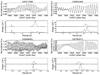 |
Fig. 1 Light curves and periodograms of CoRoT 102577568, CoRoT 102601465, CoRoT 102606401, and CoRoT 102763571 (LRa01). The origin of the CoRoT Julian day is 1 January 2000 12:00.00. |
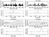 |
Fig. 2 Light curves and periodograms of CoRoT 102743567 and CoRoT 102778303 (left: LRa01, right: LRa06). |
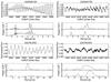 |
Fig. 3 Light curves and periodograms of CoRoT 102656730 and CoRoT 102791435 (left: LRa01, right: LRa06). |
After acquiring the data we first removed all data points marked as “bad quality” by the CoRoT pipeline. Such points are produced, for example, by the impact of high-energy particles during CoRoT passages of the South Atlantic Anomaly. Second, we normalized the light curves by dividing by the mean flux. In a final step, we detrended the light curves to remove instrumental long-term trends by subtracting a linear model. The resulting white light curves are shown in the upper panels of Figs. 1–3. For the purpose of visualization, we rebinned the light curves except that of CoRoT 102743567, which shows a particularly fast pattern of variability. In particular, we binned by a factor of 8 for light curves with a 512 s sampling rate and by a factor of 16 for those with a 32 s sampling.
For all our light curves we estimated the photometric error, σ. To this end, we divided the light curves into consecutive 0.5 d long chunks, fitted them using a second-order polynomial, and determined the standard deviation of the residuals. The mean standard deviation determined in the chunks was used as an error estimate on individual data points. The photometric error was used as an input parameter when we utilized the generalized Lomb-Scargle periodogram, which takes the photometric error of the light curve into account (see Sect. 3.3).
2.2. High-resolution spectroscopy
The spectroscopic observations of our target stars were carried out between 8 and 12 December, 2011, with the SARG echelle spectrograph, mounted on the 3.58 m “Telescopio Nazionale Galileo” (TNG) on La Palma. We used the yellow cross-disperser, which provides wavelength coverage in the 5200–7800 Å range with a gap of 150 Å at around 6200 Å caused by the separation of the CCD detectors. Our setup yields a spectral resolution of R ~ 57 000.
During our observations, weather conditions were unstable with periods of excellent conditions interrupted by rather cloudy phases. Therefore, seeing varied between 0.6′′ and 5′′. As part of our observational campaign, we also obtained a solar spectrum by observing the light reflected from the asteroid 15 Eunomia, which is required for a differential abundance analysis.
The data reduction was carried out using the REDUCE package developed by Piskunov & Valenti (2002). In particular, we performed a bias correction, order definition, extraction of the blaze function, and flat fielding. The treatment of scattered light and hot pixels is described by Piskunov & Valenti (2002). The wavelength calibration is based on ThAr-lamp reference frames and was carried out using the WAVECAL extension of REDUCE. Finally, a barycentric velocity correction was applied.
The majority of the targets was observed several times with individual exposure times between 1800 s and 3600 s. To improve the signal-to-noise ratio (S/N), we averaged all spectra taken for an individual target. For every spectrum we then computed a S/N in the 6578–6580 Å interval, which contains no strong spectral features. The resulting values are listed in Table 3 along with the total integration time. Here, the S/N refers to the averaged spectrum and although it varies across individual echelle orders and across the entire spectrum, these numbers broadly characterize the data quality. Finally, we manually continuum-normalized the spectra by dividing the flux by linear functions, which were adjusted to have the same gradient as the continuum.
3. CoRoT light curves analysis
In the upper panels of Figs. 1–3, we show the white-band CoRoT light curves of our target stars. All light curves show pronounced variability with peak-to-peak amplitudes of several percent (see Table 4), which we attribute to a rotating and temporally evolving starspot pattern.
3.1. Starspot induced color changes
To assess the plausibility of the starspot hypothesis to explain the observed variability, we examined the individual CoRoT color channels and their relation. As observed on the Sun, we postulate that the temperature of the starspots is lower than the remaining stellar photosphere (e.g., Strassmeier 2009). Once a spot appears on the visible hemisphere, the flux in all three color channels decreases. However, because the spot is cooler, the stellar spectrum appears redder. Therefore, the decrease in the blue channel flux is expected to be stronger than in the red channel. The opposite is the case, when a spot rotates off the visible hemisphere.
In Fig. 4 we show an excerpt of the white-band light curve of CoRoT 102577568 along with the ratio of the fluxes recorded in the red and blue channels. Clearly, both curves are anticorrelated. A decrease in the white light flux is accompanied by a reddening of the star, which is consistent with spot-induced photometric modulation. We verified that all investigated light curves show this behavior. Alternatively, also pulsations could cause a similar signature. Yet, typical photometric pulsation amplitudes on solar-like stars fall far behind the observed modulation (<10-5, White et al. 2011). Therefore, we conclude that the modulation in the light curves is indeed dominated by starspots with only a marginal contribution from pulsations.
3.2. Comparing LRa01 and LRa06
For half of our targets, two light curves observed about 4 yrs apart are available (see Table 2). A visual comparison of the two light curves allows to assess the temporal stability of the variability pattern. For CoRoT 102743567 and CoRoT 102778303 both the amplitude and appearance of the light curves remained unchanged. For CoRoT 102656730 this may also be the case, although it seems less clear. During the second, shorter observation, the amplitude is smaller and the pattern appears somewhat more chaotic. However, this is compatible with an observation in the low-amplitude phase of the beating pattern clearly visible during the first Long Run. The situation is similar for CoRoT 102791435, whose light curve appears more erratic, but still periodically variable during the later Long Run.
3.3. Period analysis
Clearly, the light variation of our target stars shows some periodic components. To study the variability in the frequency domain, we applied the generalized Lomb-Scargle periodogram (Zechmeister & Kürster 2009) to all light curves and show the results in the upper subfigures in the lower panels of Figs. 1–3.
All periodograms show distinguished peaks at periods between about one and twelve days. We attribute these peaks and the associated modulation in the light curve to rotating starspots and, therefore, also identify the associated period with the stellar rotation period. Generally, periodograms obtained from stellar light curves observed in LRa01 and their counterparts observed in LRa06 show similar structures. Peaks are generally less well resolved in the LRa06 periodograms, because the observation is only about half as long as the LRa01 data set.
Spectroscopic data obtained with SARG.
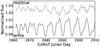 |
Fig. 4 Excerpt of the light curve of CoRoT 102577568 obtained in the white band (solid line) along with the ratio of the red- and blue-channel light curves (dashed, shifted upward by 0.025 for clarity). |
Measured peak-to-peak variability amplitude, App, and fitted rotation periods, Pfit,1 and Pfit,2.
The maximum-power periodogram peaks, which we call the primary peaks, clearly show a tendency to be accompanied by at least one nearby secondary peak. A particularly clear example for such a double-peak structure is the periodogram of CoRoT 102656730 in Fig. 3. We adopted the prewhitening procedure described by Reinhold et al. (2013) to extract closely spaced periods from the periodogram. The period associated with the primary peak was used as input for a sine, whose amplitude and phase were fitted to the data. After subtracting the resulting sine from the light curve, we computed the periodogram of the residuals. Following Reinhold et al. (2013), we examined the period space within 30% of the primary period, mainly to avoid alias periods. The resulting periodograms are shown in the lower subfigures in the lower panels of Figs. 1–3.
To determine the periods associated with the main and secondary peaks, we fitted the peaks using a Gaussian profile and used the center as an estimate of the peak location. Additionally, we interpret their FWHM as an error estimate on the location. The resulting periods and errors are listed in Table 4, and the locations of the primary and secondary peak are indicated by black vertical dots in Figs. 1–3.
In two out of the four stars observed twice by CoRoT we found that the primary and secondary peaks in the LRa06 periodograms remained at essentially the same location (CoRoT 102743567 and CoRoT 102656730). Another case is CoRoT 102778303, where the secondary peak was already quite weak in the LRa01 periodogram. The structure is mostly washed out in the LRa06 periodogram. The situation is also different for CoRoT 102791435, where the secondary peak changed in position and power, possibly indicating considerable change in the stellar spot configuration.
In the case of CoRoT 102601465, CoRoT 102606401, CoRoT 102763571 (all LRa01), and CoRoT 102791435 (LRa06) the power of the secondary peak is larger than that of the primary peak. We were able to reproduce this behavior in simulated light curves generated by the superposition of sines with a continuum of periods. Nevertheless, we interpret the secondary peak and the associated period in terms of differential rotation, but advise some caution in interpreting the result.
Results of spectral analysis with MOOG and SME.
We note that the light curves of CoRoT 102606401 and CoRoT 102601465 were also included in the study presented by Affer et al. (2012), who provide period measurements of almost two thousand stars observed by CoRoT. For CoRoT 102606401 and CoRoT 102601465, they found rotational periods of 3.039 and 6.375 days, which are compatible with our results.
3.3.1. Differential rotation
The presence of two similar periods in the periodograms of stellar light curves has been attributed to differentially rotating starspots (e.g., Reinhold et al. 2013). Differential rotation is also a possible explanation for the marked beating pattern in the light curve of CoRoT-2A (e.g., Lanza et al. 2009; Huber et al. 2010) and, therefore, also of our target stars.
On the Sun the observed latitude-dependent rotation velocity can be parametrized by  (1)where Ψ denotes the latitude, Ωeq is the equatorial angular velocity, ΔΩ = Ωeq − Ωpole is the “absolute horizontal shear”, and α is dubbed the “relative horizontal shear” (e.g., Snodgrass 1983; Reinhold et al. 2013). Similar to the situation on the Sun we may expect that the rotation rates of starspots depend not only on latitude but also on their anchoring depth. Therefore, we caution that there may not be a unique relation between latitude and starspot rotation rate as suggested by Eq. (1) and helioseismology reveals that the rotation rate of the Sun depends on both latitude and depth (Schou et al. 1998).
Therefore, if there are two measurements of Ω at two latitudes Ψ1 and Ψ2, ΔΩ can be written as  (2)Remaining ignorant of Ψ1 and Ψ2, as is often the case, a lower limit on | ΔΩ | may be obtained by assigning Ψ1 = 0° and Ψ2 = 90°, which is of course a rather unsatisfactory choice. Furthermore, attributing the larger rotational velocity measurement to the equator (Ψ = 0°), we ensure ΔΩ > 0 and thus, solar-like differential rotation. As the angular velocity is related to the rotation period P, via Ω = 2πP-1, a lower limit on the absolute and relative latitudinal shear may be obtained by
  (3)where we demand P2>P1 to endure solar-like differential rotation.
Fröhlich et al. (2009) used a three-spot model to reproduce the light curve of CoRoT-2A. Their modeling showed one slowly rotating and two fast rotating spot components. In particular, they found the length of the beating period to be compatible with the overtaking period  (4)of the slowest and the fastest differentially rotating spots. Tentatively assigning the primary and secondary peaks identified in the periodograms to differentially rotating spots, we used Eq. (3) to derive lower limits for the absolute and relative horizontal shear and Eq. (4) to estimate the beating period; the values are listed in Table 4.
In our data, the beating period is not always well defined. Some light curves do not fully cover a pattern as is the case for CoRoT 102601465 (Fig. 1) and the definition of the start and end of a cycle remains somewhat ambiguous. Nonetheless, the calculated beating periods are in reasonable agreement with the observed behavior in the light curves. In CoRoT 102743567, a number of beating cycles with different duration was observed and the beating structure persisted over (or reappeared after) four years. If attributable to differential rotation, this indicates varying relative spot velocities. Given a temporally constant and unique mapping between latitude and velocity, this implies changing spot latitudes.
4. Spectral analysis
We determined the stellar parameters using two complementary approaches. First, the curve-of-growth based MOOG package (Sneden 1973) and, second, the Spectroscopy Made Easy (SME) package presented by Valenti & Piskunov (1996), which relies on direct spectral modeling. A visual inspection of the spectra with regard to double line profiles did not reveal indications for binarity in any of our target stars.
4.1. Stellar parameter determination using MOOG
The stellar atmospheric parameters effective temperature (Teff), surface gravity (log g), metallicity ([Fe/H]), and microturbulence velocity (ξmic) were derived using the 2014 version of MOOG3 and a grid of 1D Kurucz ATLAS9 model atmospheres4 (Kurucz 1993). Additionally, we used PYSPEC, a Python interface to run MOOG (Bubar & King 2010).
The analysis carried out by MOOG relies on a curve-of-growth approach in which the stellar atmospheric equilibrium is adjusted to match equivalent width (EW) measurements (see also Gray 2005). To adjust the equilibrium and find the stellar parameters, it is essential to measure the EWs of lines originating from a single element in different ionization states. For low-mass stars, iron provides a plethora of Fe i and Fe ii lines distributed over the optical spectral range; the Fe ii lines, however, are usually more scarce. Our choice of Fe i and Fe ii lines is based on the final line list5 provided by Sousa et al. (2008), who present a total of 263 Fe i and 36 Fe ii lines, together with their excitation potentials and oscillator strengths in the wavelength range between 4500 Å and 6900 Å. We scrutinized their line list and eliminated lines not usable in our analysis, for example, lines suffering from heavy blending or lines for which we could not derive adequate continua to obtain the EW. Additionally, we neglected weak lines (≲5 mÅ) and lines in wavelength intervals with low S/N. The number of the remaining Fe i and Fe ii lines of each star are listed in Table 5.
Equivalent widths were measured by fitting the line profiles using a Gaussian. The local continuum was adjusted manually for each line to achieve the optimal normalization. To this end, a solar model spectrum served as a comparison, which we also used for the unambiguous line identification in the observed spectra. For CoRoT 102743567 no EWs could be determined from our spectra owing to extreme rotational broadening (≈64 km s-1, see Sect. 4.2 and Table 5).
To minimize the impact of uncertainties in the atomic line parameters and the characteristics of our particular instrumental setup on the analysis, we carried out a differential abundance analysis. Abundances are thus defined with respect to the Sun ![Mathematical equation: \begin{equation} [\mathrm{Fe/H}] = \mathrm{log} \left(\frac{N(\mathrm{Fe})}{N(\mathrm{H})}\right)_* - \mathrm{log} \left( \frac{N(\mathrm{Fe})}{N(\mathrm{H})} \right)_{\odot},\quad \log\, N(\mathrm{H}) \equiv 12. \end{equation}](/articles/aa/full_html/2016/06/aa27508-15/aa27508-15-eq169.png) (5)Therefore, we determined the EWs of our sample of spectral lines in a solar spectrum, which we obtained by observing light reflected off the asteroid 15 Eunomia with the same instrumental setup. Our results are summarized in Table 5.
(5)Therefore, we determined the EWs of our sample of spectral lines in a solar spectrum, which we obtained by observing light reflected off the asteroid 15 Eunomia with the same instrumental setup. Our results are summarized in Table 5.
In MOOG, errors were estimated by studying various correlations. In particular, the temperature value was varied until the correlation between excitation potential and the Fe i abundances reached the 1σ level. The error on the microturbulence velocity was derived equivalently by adapting it until the correlation between the abundances and the reduced EWs6 reached 1σ. In MOOG, the surface gravity is determined by minimizing the difference between the abundances obtained from the Fe i and Fe ii lines. Yet, the abundances depend on the stellar parameters including the surface gravity, which implies that the error on the surface gravity depends on the surface gravity itself. Therefore, the error had to be derived in an iterative process, which is described in detail by Bubar & King (2010).
4.2. Stellar parameter determination using SME
Following the analysis with MOOG, we used the software package SME in version 2.1 to derive a complementary set of parameters. In contrast to MOOG, the technique employed by SME is based on fitting synthetic spectra to the observations. As input, a grid of model atmospheres and an atomic line list are required. For the latter we obtained atomic data from VALD37 (Kupka et al. 2000) and, again, used ATLAS9 Kurucz atmospheres.
In our analysis, we used SME to fit individual echelle orders neglecting the low S/N edges of the orders and other unsuitable spectral regions. The latter comprise sections with spectral lines missing in the line list; regions affected by cosmics, telluric lines, airglow emission lines, and bands lacking any notable stellar absorption lines.
In our fits, we used the values for Teff, log g, [Fe/H], and ξmic determined with MOOG as initial values for the SME fit. For the macroturbulence parameters, we assumed the solar value of ξmac = 3.57 km s-1. In a first fitting step, we determined the radial velocity shift νrad for all orders. We averaged the results in the different orders and interpreted the mean as the best estimate of the stellar parameter and its standard deviation as a robust error estimate. Second, we determined the mean rotational broadening parameter, ν sin i, in the same manner. In a third step, we fitted ξmic and [M/H], and finally, fitted Teff and log g. During the fitting process, all parameters not currently fitted remained fixed at their best-fit values. The final values are summarized in Table 5. An example of a spectral interval of CoRoT 102656730 is shown together with the best-fit synthetic spectrum in Fig. 5.
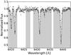 |
Fig. 5 Segment of the observed (open squares) and synthetic spectrum (solid line) of CoRoT 102656730. The grey shaded regions were used to determine the stellar parameters. |
In the case of CoRoT 102743567 we fitted νrad and ν sin i using only orders covering the strong Hα Balmer line and the Na i doublet at ≈5990 Å. As initial values we calculated Teff photometrically using B − V colors as described in Sect. 4.4. Furthermore, we chose typical values of main-sequence stars for log g = 4.3 based on Gray (2005), solar metallicity, and ξmic = 1.5 km s-1.
4.3. Stellar parameters obtained using MOOG and SME
In general, we find good agreement between the effective temperatures, surface gravities, metallicities, and microturbulence velocities derived with SME and MOOG. With a few exceptions, the values agree within their respective uncertainties. However, the surface gravities found with SME are systematically higher than those determined with MOOG. In particular, we find differences between 0.12 and 0.37 for all stars but CoRoT 102778303 for which the deviation reaches 0.88; however, the error is also large. This star is the coolest in our sample, and we speculate that the line EW measurements may be affected by line blends, which could also account for the rather low metallicity of −0.54 ± 0.05 found in our MOOG analysis. The direct fitting approach implemented in SME should minimize errors caused by blending effects or continuum determination.
Valenti & Fischer (2005) analyzed 1040 F, G, and K stars using SME and obtained statistical errors of 44 K on Teff, 0.06 on log g, and 0.03 on the metallicity. In our analysis, we found that the deviation among fits to individual echelle orders were larger than their estimates. Thus, our SME errors are likely dominated by systematics.
All stars show substantial photometric variability, which we attribute to starspots. Therefore, high starspot coverage fractions are conceivable (e.g., Huber et al. 2010), although we caution that the data have not been taken simultaneously. A high starspot coverage fraction may actually challenge the assumption of a single-temperature photosphere, which tacitly underlies our spectral analysis. It may also explain at least a fraction of the differences between the MOOG and SME analysis.
4.4. Color, extinction, and distance
Ramírez & Meléndez (2005) provide metallicity-dependent relations between color and effective temperature. Given the spectroscopically determined parameters and the observed B − V colors (see Table 1), we can determine the B − V color excess. The resulting intrinsic colors, (B − V)0, and excesses, E(B − V), are given in Table 6. In the conversion, we applied the effective temperatures and metallicities derived using MOOG (Table 5) and assumed main-sequence stars. By substituting the upper and lower error boundaries on the effective temperature, we estimated that the temperature-induced error on the color excess is on the order of 0.03 mag.
For the star CoRoT 102743567, for which no spectroscopic parameters could be determined, we used the observed B − V color of 0.39 mag to obtain an estimate of 7000 K for its effective temperature, which points to an early F-type star. We note that B − V = 0.39 mag requires a slight stretch of the Ramírez & Meléndez (2005) calibration, which is formally only valid until 0.4. This result is consistent with the classification as an A9III type star by Sebastian et al. (2012) based on low-resolution spectroscopy.
We proceeded by converting the color excess into optical extinction by multiplying with R, for which we assumed a value of 3.1 (Predehl & Schmitt 1995). Using Table 15.7 from Cox (2000), we estimated absolute visual magnitudes based on our effective temperature determinations and, finally, calculated a photometric distance estimate for our target stars, taking the extinction into account. Estimating an accuracy of ±0.5 mag for the distance modulus, the typical error on the distances is 25%.
4.5. Age of the sample stars
The Li i resonance doublet at 6707.76 Å and 6707.91 Å can be used as an age estimator in young stars because lithium depletion progresses quickly during the first few hundred Myr (e.g., Soderblom 2010). In Fig. 6, we show the spectral region around the Li i line for our sample stars. Unambiguous detections are present for four out of the eight targets. In a quantitative analysis, we fitted the line profile by a Gaussian after adjusting the local continuum, which is the main source of error.
Clear detections of the lithium line were obtained in CoRoT 102577568, CoRoT 102601465, CoRoT 102606401, and CoRoT 102763571. A formally significant line detection is also obtained in CoRoT 102778303. We caution, however, that this result may require confirmation at higher S/N. For CoRoT 102656730 and CoRoT 102791435 we derived upper limits on the line EW. To this end, we generated artificial data sets between 6707.0 Å and 6708.5 Å assuming that no line is present and fitted them using the model including the absorption line. Repeating this experiment 10 000 times, we determined the distribution of line EW measurements given that in reality no line exists and give the 90% cut-off as the upper limit for a significant detection. The final EWs along with their 90% confidence intervals are listed in Table 7.
Intrinsic color, color excess, and photometric distance estimate.
The Li i line is known to be blended by an Fe i line at 6707.43 Å, which has not been taken into account in our fitting. Favata et al. (1993) studied the contribution of this iron line to the overall EW. From their Fig. 1, we estimate that the contribution for a star with an effective temperature of 5500 K should be on the order of 10 mÅ and it decreases toward higher temperatures. However, for CoRoT 102778303, at a temperature of about 4700 K, the Fe i line could have an EW of about 20 mÅ, which is on the same order as our measurement. While this could indicate that the line may indeed be attributable to iron, this seems unlikely given the subsolar abundance pattern. All other detections should, if anything, be affected on the 10% level, casting no doubt on the detection of the Li i line itself.
We proceeded by comparing the measured Li i line EWs with measurements in open cluster members of well-known age. In Fig. 7 we show our Li i EW measurements as a function of effective temperature along with results for the open clusters Orion Ic (10 Myr, King 1993), NGC 2264 (10 Myr, Soderblom et al. 1999), Pleiades (100 Myr, Soderblom et al. 1993b), Ursa Major (300 Myr, Soderblom et al. 1993c), Hyades (660 Myr, Soderblom et al. 1990), and Praesepe (660 Myr, Soderblom et al. 1993a). Based on their location in the plot, we arrived at the age estimates provided in Table 7. Although the stars within an open cluster are formed simultaneously, there is a considerable scatter around a mean value in the measured EWs for a given effective temperature.
Equivalent widths of Li i line and stellar age estimates.
As a result of the well-established age-activity-rotation paradigm (e.g., Skumanich 1972), rotation itself can be used as an age indicator. We calculated the stellar ages of our target stars based on gyrochronological models presented by Barnes (2007; their Eq. (3)). In particular, we used the rotation period and the intrinsic color (B − V)0 as input parameters. The errors were estimated using their Eq. (16). Again, we present our results in Table 7.
Almost all of the gyrochronological estimates are consistent with our estimates based on the comparison with open clusters. The single exception is CoRoT 102778303 for which our cluster comparison yields a higher age. However, the star CoRoT 102778303 is the coolest target in our sample, for which we obtained effective temperature estimates of 4840 ± 100 K with MOOG and 4680 ± 150 K with SME. If the star is at the lower edge of the indicated temperature range and the Li i line is not heavily contaminated by iron, its age could also be compatible with that of the Pleiades in Fig. 7.
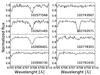 |
Fig. 6 Normalized spectra of our target stars showing the wavelength region around the Li i line at 6708 Å. |
5. Discussion
5.1. Stellar parameters and age determination
The results of our spectral analysis are broadly consistent with the classification provided by Exo-Dat (see Table 1).
All stars show gyrochronological ages between 111 and 418 Myr. Additionally, five stars show a Li i line supporting a low age, although the detection in CoRoT 102778303 remains somewhat ambiguous. Fast rotation and young age are compatible with high levels of activity and large starspot coverage fractions responsible for the photometric variability. Judging from the derived spectroscopic parameters, our sample consists of main-sequence stars. However, we find that the luminosity class for CoRoT 102778303 provided by Exo-Dat is probably inappropriate. The obtained log g and ν sin i values, gyrochronology, and rotation period indicate that CoRoT 102778303 should be classified as a dwarf instead of a subgiant.
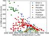 |
Fig. 7 Li i EW vs. effective temperature for several open clusters. The location of our sample stars is indicated by black circles (effective temperatures derived with MOOG). |
5.2. Differential rotation, spot evolution, and flip-flop events
Reinhold et al. (2013) studied differential rotation in a sample of 40 661 active stars observed by Kepler. In this sample, 77.2% of the targets show a second periodogram peak, which they attribute to a second rotation period. Following their interpretation, we show our results for the lower limit of the relative horizontal shear in the context of the sample presented by Reinhold et al. (2013) in Fig. 8. Our values are clearly compatible with theirs, although CoRoT 102601465 lies near their detection limit. In particular, we were able to confirm the trend of increasing relative shear, α, with higher rotation periods. CoRoT 102778303 and CoRoT 102791435, the coolest targets with the longest rotation period which have been observed twice, show a considerable shift in the value of the relative shear parameter between the two observation epochs roughly four years apart. We attribute the difference to both an uncertainty resulting from the prewhitening technique and the variability of the spot configuration. The results reflect the uncertainty that is expected in individual measurements.
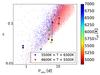 |
Fig. 8 Lower limits of the relative horizontal shear as a function of Pmin for our target stars and the sample of Reinhold et al. (2013). Values determined for stars with two CoRoT light curves obtained during different epochs are connected by a solid line. We adopted the effective temperatures derived with MOOG and used 7000 K for CoRoT 102743567. |
The star CoRoT 102743567 is the earliest star and fastest rotator in our sample. Combining a canonical radius of 1.5 R⊙ for the star (Cox 2000) with the rotation period, we estimate an equatorial rotation velocity, νeq, of 90–100 km s-1. Based on our period analysis, we further estimated a relative horizontal shear parameter of 0.052. Ammler-von Eiff & Reiners (2012) studied differential rotation specifically in A- and F-type stars using line profile analyses. Although the authors find that the fraction of differential rotators decreases both as a function of increasing temperature and rotation velocity, about 10% of their sample stars with ν sin i ≈ 100 km s-1 show measurable differential rotation. Among these stars, a relative horizontal shear of ≈0.05 seems too moderate (see their Fig. 10). Indeed, at 7000 K an absolute horizontal shear, ΔΩ, of 0.6 rad d-1 may be expected, which is also quite compatible with our value of 0.4 rad d-1. We note that the spectral type of CoRoT 102743567 is in the range of γ Dor-type variables, which show pulsations with periods on the order of one day (Kaye et al. 1999; Zwintz et al. 2013). Although it is still hard to unambiguously distinguish between the rotational modulation and a potential pulsational component (cf., Zwintz et al. 2013), our results are consistent with dominant rotational variation.
If the beating pattern is to be caused by differentially rotating active regions (alone), its length also defines a minimal lifetime for the associated regions, which in our case ranges between 15 d and about 150 d. Typical sunspot lifetimes are on the order of or less than one month (Solanki 2003) and low- to mid-latitude spots on rapidly rotating, young single main-sequence stars also appear to have lifetimes of about one month (Hussain 2002). Therefore, the longer beating periods seem challenging in terms of spot lifetimes. However, larger spots tend to have longer lifetimes (Solanki 2003).
The light curves of our sample stars (Figs. 1–3) show a similar pattern of variability to the light curves of flip-flop stars such as the active giant FK Com or young solar analogs (see Jetsu et al. 1993; Berdyugina & Järvinen 2005; Oláh et al. 2006; Hackman et al. 2013). Flip-flops are a specific manifestation of spot evolution, characterized by alternating spot coverage on two long-lived active longitudes on opposing hemispheres, which requires “coordinated” spot evolution. While the origin of the phenomenon may be entirely explained by the evolution of quasi-stationary spots, differential rotation and latitudinal spot migration may also play a role or even largely explain the observations (Jetsu et al. 1993; Hackman et al. 2013).
The surface reconstructions of CoRoT-2 have revealed spot concentrations on active longitude on opposing hemispheres (Lanza et al. 2009; Huber et al. 2010), which alternate in strength on the beating timescale (≈50 d). Owing to the similarity of the light curves studied here, a comparable behavior may be expected. While the behavior of the light curves analyzed here is reminiscent of the flip-flop phenomenon, the flip-flop timescales observed so far are several years (e.g., Hackman et al. 2013). For instance, Jetsu et al. (1993) detected only three flip-flop events in a photometric data set spanning roughly 25 yr. While spot evolution certainly contributes to the morphology of the observed light curves, the absence of differential rotation in our late-type sample stars appears unlikely.
6. Summary and conclusion
We present a photometric and spectroscopic study of eight stars with light curves showing photometric variability similar to that of CoRoT-2A. The sample spans a wide range of spectral types from early F- to mid K-type. The stellar parameters obtained from our spectral analysis with SME and MOOG are generally consistent. For the fastest rotator in our sample, CoRoT 102743567, no detailed spectral analysis could be carried out. For the remaining stars, we obtained surface gravities compatible with that of main-sequence stars. Combining the spectroscopically derived effective temperatures with the stellar colors, we deduced distances corrected for interstellar reddening.
The light curve analysis showed large photometric amplitudes of up to 7.5% and short rotation periods between about 0.8 d and 11 d. We found the photometric variability to be consistent with rotational modulation by starspots. In the majority of cases, our periodogram analysis revealed two peaks corresponding to similar periods, whose spacing is related to the beating period. Attributing the two periods to differentially rotating spots and combining the results with our spectroscopic measurements, we find results consistent with similar previous analyses of Kepler light curves (Reinhold et al. 2013). However, in the end it remains unclear whether the prominent pattern of variability exhibited by the light curves is dominated by differential rotation or spot evolution. In analogy to findings from photometric campaigns of the active giant FK Com, we expect both effects to play a role.
Gyrochronological models show that all sample stars in our sample are young dwarfs (100–400 Myr). In four stars, we also found detectable Li i absorption, which also points toward a low age. This is consistent with the high level of activity evident in the light curves. Our sample shows a wide spread in spectral types including F-, G-, and K-type stars, which all show a similar photometric beating behavior. This suggests that all low-mass stars with outer convection zones may produce a similar CoRoT-2A-like light curve sometime in their early evolution.
The values in Table 1 are rounded. The exact numbers including uncertainties can be found at http://cesam.oamp.fr/exodat/
The Kurucz grids of model atmospheres can be found at http://kurucz.harvard.edu/grids.html
The line list is available online at http://www.astro.up.pt/~sousasag/ares
The EW divided by the line wavelength.
VALD3 is available at http://vald.astro.uu.se/
Acknowledgments
The authors thank Dr. Sebastian Schröter for valuable discussions in preparing the project and support in obtaining the spectra. This work was prepared using PyAstronomy. This research has also made use of the ExoDat Database, operated at LAM-OAMP, Marseille, France, on behalf of the CoRoT/Exoplanet program. We acknowledge use of observational data obtained with SARG at the TNG, Roque de Los Muchachos, Spain. This work has made use of the VALD database, operated at Uppsala University, the Institute of Astronomy RAS in Moscow, and the University of Vienna. Special thanks to Eric J. Bubar (University of Rochester) for making his MSPAWN and PYSPEC codes available to us. We are grateful to Nikolai Piskunov (University of Uppsala) for providing SME to us. We made use of the stellar spectrum synthesis program SPECTRUM of Richard O. Gray (Appalachian State University).
References
- Affer, L., Micela, G., Favata, F., & Flaccomio, E. 2012, MNRAS, 424, 11 [NASA ADS] [CrossRef] [Google Scholar]
- Alonso, R., Auvergne, M., Baglin, A., et al. 2008, A&A, 482, L21 [NASA ADS] [CrossRef] [EDP Sciences] [Google Scholar]
- Ammler-von Eiff, M., & Reiners, A. 2012, A&A, 542, A116 [NASA ADS] [CrossRef] [EDP Sciences] [Google Scholar]
- Auvergne, M., Bodin, P., Boisnard, L., et al. 2009, A&A, 506, 411 [NASA ADS] [CrossRef] [EDP Sciences] [Google Scholar]
- Baglin, A., Auvergne, M., Boisnard, L., et al. 2006, in COSPAR Meeting, 36, 36th COSPAR Scientific Assembly, 3749 [Google Scholar]
- Barnes, S. A. 2007, ApJ, 669, 1167 [NASA ADS] [CrossRef] [Google Scholar]
- Berdyugina, S. V., & Tuominen, I. 1998, A&A, 336, L25 [NASA ADS] [Google Scholar]
- Berdyugina, S. V., & Järvinen, S. P. 2005, Astron. Nachr., 326, 283 [NASA ADS] [CrossRef] [Google Scholar]
- Berdyugina, S. V., Moss, D., Sokoloff, D., & Usoskin, I. G. 2006, A&A, 445, 703 [NASA ADS] [CrossRef] [EDP Sciences] [Google Scholar]
- Bouchy, F., Queloz, D., Deleuil, M., et al. 2008, A&A, 482, L25 [NASA ADS] [CrossRef] [EDP Sciences] [Google Scholar]
- Bubar, E. J., & King, J. R. 2010, AJ, 140, 293 [NASA ADS] [CrossRef] [Google Scholar]
- Cox, A. N. 2000, Allen’s astrophysical quantities (New York: AIP Press) [Google Scholar]
- Czesla, S., Huber, K. F., Wolter, U., Schröter, S., & Schmitt, J. H. M. M. 2009, A&A, 505, 1277 [NASA ADS] [CrossRef] [EDP Sciences] [Google Scholar]
- Deleuil, M., Meunier, J. C., Moutou, C., et al. 2009, AJ, 138, 649 [NASA ADS] [CrossRef] [Google Scholar]
- Favata, F., Barbera, M., Micela, G., & Sciortino, S. 1993, A&A, 277, 428 [NASA ADS] [Google Scholar]
- Fröhlich, H.-E., Küker, M., Hatzes, A. P., & Strassmeier, K. G. 2009, A&A, 506, 263 [NASA ADS] [CrossRef] [EDP Sciences] [Google Scholar]
- Gray, D. F. 2005, The Observation and Analysis of Stellar Photospheres (Cambridge, UK: Cambridge University Press) [Google Scholar]
- Grevesse, N., Asplund, M., & Sauval, A. J. 2007, Space Sci. Rev., 130, 105 [Google Scholar]
- Guillot, T., & Havel, M. 2011, A&A, 527, A20 [NASA ADS] [CrossRef] [EDP Sciences] [Google Scholar]
- Hackman, T., Pelt, J., Mantere, M. J., et al. 2013, A&A, 553, A40 [NASA ADS] [CrossRef] [EDP Sciences] [Google Scholar]
- Huber, K. F., Czesla, S., Wolter, U., & Schmitt, J. H. M. M. 2010, A&A, 514, A39 [NASA ADS] [CrossRef] [EDP Sciences] [Google Scholar]
- Hussain, G. A. J. 2002, Astron. Nachr., 323, 349 [NASA ADS] [CrossRef] [Google Scholar]
- Järvinen, S. P., Berdyugina, S. V., & Strassmeier, K. G. 2005, A&A, 440, 735 [NASA ADS] [CrossRef] [EDP Sciences] [Google Scholar]
- Jenkins, J. M., Caldwell, D. A., Chandrasekaran, H., et al. 2010, ApJ, 713, L120 [NASA ADS] [CrossRef] [Google Scholar]
- Jetsu, L., Pelt, J., & Tuominen, I. 1993, A&A, 278, 449 [NASA ADS] [Google Scholar]
- Karoff, C., Campante, T. L., Ballot, J., et al. 2013, ApJ, 767, 34 [NASA ADS] [CrossRef] [Google Scholar]
- Kaye, A. B., Handler, G., Krisciunas, K., Poretti, E., & Zerbi, F. M. 1999, PASP, 111, 840 [NASA ADS] [CrossRef] [Google Scholar]
- King, J. R. 1993, AJ, 105, 1087 [NASA ADS] [CrossRef] [Google Scholar]
- Kupka, F. G., Ryabchikova, T. A., Piskunov, N. E., Stempels, H. C., & Weiss, W. W. 2000, Balt. Astron., 9, 590 [NASA ADS] [Google Scholar]
- Kurucz, R. L. 1993, SYNTHE spectrum synthesis programs and line data (Cambridge: SAO) [Google Scholar]
- Lanza, A. F., Pagano, I., Leto, G., et al. 2009, A&A, 493, 193 [NASA ADS] [CrossRef] [EDP Sciences] [Google Scholar]
- Oláh, K., Korhonen, H., Kővári, Z., Forgács-Dajka, E., & Strassmeier, K. G. 2006, A&A, 452, 303 [NASA ADS] [CrossRef] [EDP Sciences] [Google Scholar]
- O’Neal, D., Saar, S. H., & Neff, J. E. 1996, ApJ, 463, 766 [NASA ADS] [CrossRef] [Google Scholar]
- Piskunov, N. E., & Valenti, J. A. 2002, A&A, 385, 1095 [NASA ADS] [CrossRef] [EDP Sciences] [Google Scholar]
- Piskunov, N. E., Tuominen, I., & Vilhu, O. 1990, A&A, 230, 363 [NASA ADS] [Google Scholar]
- Predehl, P., & Schmitt, J. H. M. M. 1995, A&A, 293, 889 [NASA ADS] [Google Scholar]
- Ramírez, I., & Meléndez, J. 2005, ApJ, 626, 465 [NASA ADS] [CrossRef] [Google Scholar]
- Reinhold, T., Reiners, A., & Basri, G. 2013, A&A, 560, A4 [NASA ADS] [CrossRef] [EDP Sciences] [Google Scholar]
- Rodono, M., Cutispoto, G., Pazzani, V., et al. 1986, A&A, 165, 135 [NASA ADS] [Google Scholar]
- Schou, J., Antia, H. M., Basu, S., et al. 1998, ApJ, 505, 390 [NASA ADS] [CrossRef] [Google Scholar]
- Schröter, S., Czesla, S., Wolter, U., et al. 2011, A&A, 532, A3 [NASA ADS] [CrossRef] [EDP Sciences] [Google Scholar]
- Sebastian, D., Guenther, E. W., Schaffenroth, V., et al. 2012, A&A, 541, A34 [NASA ADS] [CrossRef] [EDP Sciences] [Google Scholar]
- Skumanich, A. 1972, ApJ, 171, 565 [NASA ADS] [CrossRef] [Google Scholar]
- Sneden, C. A. 1973, Ph.D. Thesis, The University of Texas at Austin [Google Scholar]
- Snodgrass, H. B. 1983, ApJ, 270, 288 [NASA ADS] [CrossRef] [Google Scholar]
- Soderblom, D. R. 2010, ARA&A, 48, 581 [NASA ADS] [CrossRef] [Google Scholar]
- Soderblom, D. R., Oey, M. S., Johnson, D. R. H., & Stone, R. P. S. 1990, AJ, 99, 595 [NASA ADS] [CrossRef] [Google Scholar]
- Soderblom, D. R., Fedele, S. B., Jones, B. F., Stauffer, J. R., & Prosser, C. F. 1993a, AJ, 106, 1080 [NASA ADS] [CrossRef] [Google Scholar]
- Soderblom, D. R., Jones, B. F., Balachandran, S., et al. 1993b, AJ, 106, 1059 [NASA ADS] [CrossRef] [Google Scholar]
- Soderblom, D. R., Pilachowski, C. A., Fedele, S. B., & Jones, B. F. 1993c, AJ, 105, 2299 [NASA ADS] [CrossRef] [Google Scholar]
- Soderblom, D. R., King, J. R., Siess, L., Jones, B. F., & Fischer, D. 1999, AJ, 118, 1301 [NASA ADS] [CrossRef] [Google Scholar]
- Solanki, S. K. 2003, A&A Rev., 11, 153 [NASA ADS] [CrossRef] [Google Scholar]
- Sousa, S. G., Santos, N. C., Mayor, M., et al. 2008, A&A, 487, 373 [NASA ADS] [CrossRef] [EDP Sciences] [MathSciNet] [Google Scholar]
- Strassmeier, K. G. 2009, A&ARv, 17, 251 [NASA ADS] [CrossRef] [Google Scholar]
- Valenti, J. A., & Fischer, D. A. 2005, ApJS, 159, 141 [NASA ADS] [CrossRef] [MathSciNet] [Google Scholar]
- Valenti, J. A., & Piskunov, N. 1996, A&AS, 118, 595 [NASA ADS] [CrossRef] [EDP Sciences] [Google Scholar]
- White, T. R., Bedding, T. R., Stello, D., et al. 2011, ApJ, 743, 161 [NASA ADS] [CrossRef] [Google Scholar]
- Zechmeister, M., & Kürster, M. 2009, A&A, 496, 577 [NASA ADS] [CrossRef] [EDP Sciences] [Google Scholar]
- Zwintz, K., Fossati, L., Ryabchikova, T., et al. 2013, A&A, 550, A121 [NASA ADS] [CrossRef] [EDP Sciences] [Google Scholar]
All Tables
Measured peak-to-peak variability amplitude, App, and fitted rotation periods, Pfit,1 and Pfit,2.
All Figures
|
Fig. 1 Light curves and periodograms of CoRoT 102577568, CoRoT 102601465, CoRoT 102606401, and CoRoT 102763571 (LRa01). The origin of the CoRoT Julian day is 1 January 2000 12:00.00. |
| In the text | |
|
Fig. 2 Light curves and periodograms of CoRoT 102743567 and CoRoT 102778303 (left: LRa01, right: LRa06). |
| In the text | |
|
Fig. 3 Light curves and periodograms of CoRoT 102656730 and CoRoT 102791435 (left: LRa01, right: LRa06). |
| In the text | |
|
Fig. 4 Excerpt of the light curve of CoRoT 102577568 obtained in the white band (solid line) along with the ratio of the red- and blue-channel light curves (dashed, shifted upward by 0.025 for clarity). |
| In the text | |
|
Fig. 5 Segment of the observed (open squares) and synthetic spectrum (solid line) of CoRoT 102656730. The grey shaded regions were used to determine the stellar parameters. |
| In the text | |
|
Fig. 6 Normalized spectra of our target stars showing the wavelength region around the Li i line at 6708 Å. |
| In the text | |
|
Fig. 7 Li i EW vs. effective temperature for several open clusters. The location of our sample stars is indicated by black circles (effective temperatures derived with MOOG). |
| In the text | |
|
Fig. 8 Lower limits of the relative horizontal shear as a function of Pmin for our target stars and the sample of Reinhold et al. (2013). Values determined for stars with two CoRoT light curves obtained during different epochs are connected by a solid line. We adopted the effective temperatures derived with MOOG and used 7000 K for CoRoT 102743567. |
| In the text | |
Current usage metrics show cumulative count of Article Views (full-text article views including HTML views, PDF and ePub downloads, according to the available data) and Abstracts Views on Vision4Press platform.
Data correspond to usage on the plateform after 2015. The current usage metrics is available 48-96 hours after online publication and is updated daily on week days.
Initial download of the metrics may take a while.