| Issue |
A&A
Volume 590, June 2016
|
|
|---|---|---|
| Article Number | A9 | |
| Number of page(s) | 15 | |
| Section | Galactic structure, stellar clusters and populations | |
| DOI | https://doi.org/10.1051/0004-6361/201526765 | |
| Published online | 28 April 2016 | |
FORS2/VLT survey of Milky Way globular clusters
II. Fe and Mg abundances of 51 Milky Way globular clusters on a homogeneous scale⋆,⋆⋆
1
European Southern Observatory, Alonso de Córdova 3107, Santiago, Chile
e-mail: bdias@eso.org
2
Universidade de São Paulo, Dept. de Astronomia, Rua do Matão 1226,
05508-090
São Paulo,
Brazil
3
Department of Physics, Durham University,
South Road, Durham
DH1 3LE,
UK
4
INAF, Osservatorio Astronomico di Padova,
Vicolo dell’Osservatorio 5,
35122
Padova,
Italy
5
Research School of Astronomy & Astrophysics, Australian
National University, Mount Stromlo Observatory, via Cotter Road, Weston Creek, ACT
2611,
Australia
6
Università di Padova, Dipartimento di Astronomia,
Vicolo dell’Osservatorio 2,
35122
Padova,
Italy
7
Instituto de Astrofísica, Pontificia Universidad Católica de
Chile, Av. Vicuña Mackenna 4860,
782-0436 Macul, Santiago, Chile
8
Millennium Institute of Astrophysics, Av. Vicuña Mackenna 4860, 782-0436 Macul,
Santiago,
Chile
9
Museo Interactivo Mirador, Dirección de Educación,
Av. Punta Arenas, 6711 La Granja,
Santiago,
Chile
Received: 16 June 2015
Accepted: 29 February 2016
Context. Globular clusters trace the formation and evolution of the Milky Way and surrounding galaxies, and outline their chemical enrichment history. To accomplish these tasks it is important to have large samples of clusters with homogeneous data and analysis to derive kinematics, chemical abundances, ages and locations.
Aims. We obtain homogeneous metallicities and α-element enhancement for 51 Galactic bulge, disc, and halo globular clusters that are among the most distant and/or highly reddened in the Galaxy’s globular cluster system. We also provide membership selection based on stellar radial velocities and atmospheric parameters. The implications of our results are discussed.
Methods. We observed R ~ 2000 spectra in the wavelength interval 456–586 nm for over 800 red giant stars in 51 Galactic globular clusters. We applied full spectrum fitting with the code ETOILE together with libraries of observed and synthetic spectra. We compared the mean abundances of all clusters with previous work and with field stars. We used the relation between mean metallicity and horizontal branch morphology defined by all clusters to select outliers for discussion.
Results. [Fe/H], [Mg/Fe], and [α/Fe] were derived in a consistent way for almost one-third of all Galactic globular clusters. We find our metallicities are comparable to those derived from high-resolution data to within σ = 0.08 dex over the interval −2.5< [Fe/H] < 0.0. Furthermore, a comparison of previous metallicity scales with our values yields σ< 0.16 dex. We also find that the distribution of [Mg/Fe] and [α/Fe] with [Fe/H] for the 51 clusters follows the general trend exhibited by field stars. It is the first time that the following clusters have been included in a large sample of homogeneous stellar spectroscopic observations and metallicity derivation: BH 176, Djorg 2, Pal 10, NGC 6426, Lynga 7, and Terzan 8. In particular, only photometric metallicities were available previously for the first three clusters, and the available metallicity for NGC 6426 was based on integrated spectroscopy and photometry. Two other clusters, HP 1 and NGC 6558, are confirmed as candidates for the oldest globular clusters in the Milky Way.
Conclusions. Stellar spectroscopy in the visible at R ~ 2000 for a large sample of globular clusters is a robust and efficient way to trace the chemical evolution of the host galaxy and to detect interesting objects for follow-up at higher resolution and with forthcoming giant telescopes. The technique used here can also be applied to globular cluster systems in nearby galaxies with current instruments and to distant galaxies with the advent of ELTs.
Key words: stars: abundances / stars: kinematics and dynamics / stars: Population II / Galaxy: stellar content / Galaxy: evolution / globular clusters: general
Based on observations collected at the European Southern Observatory/Paranal, Chile, under programmes 68.B-0482(A), 69.D-0455(A), 71.D-0219(A), 077.D-0775(A), and 089.D-0493(B).
Full Tables 1 and A.2 with the derived average parameters for the 758 red giant stars are only available at the CDS via anonymous ftp to cdsarc.u-strasbg.fr (130.79.128.5) or via http://cdsarc.u-strasbg.fr/viz-bin/qcat?J/A+A/590/A9
© ESO, 2016
1. Introduction
One of the most important questions about our Universe is, How did galaxies form and evolve? A useful approach is to observe stars of different ages and stellar populations that have imprinted in their kinematics and chemical abundances the signatures of their formation period. Globular clusters are fossils tracing formation processes of their host galaxies at early epochs (~10–13 Gyr ago) and of more recent processes involving mergers with satellite galaxies.
Understanding the system of Galactic globular clusters (GGCs) is of prime importance to build up a picture of the formation and early evolution of the Milky Way. Cluster ages are used to place the GGCs in the chronology of our Galaxy; the evolution of their chemical abundances and kinematics provides evidence for the dynamical and chemical evolution of the protogalactic halo and bulge.
With the advent of multifibre spectrographs used in 8 m class telescopes, high-resolution spectra of sufficient signal-to-noise ratio (S/N) can now be obtained for the cluster giant stars out to (m − M)V ≈ 19, i.e. for >80% of the GGCs. Nevertheless, the largest homogeneous samples of metallicities are still based on low-resolution spectroscopy (and calibrated with high spectral resolution results). Even so, more than 50% of GGCs do not have any spectroscopic estimation of their [Fe/H] (see Saviane et al. 2012b for a review of [Fe/H] values available in the literature).
Homogeneous determinations of [Fe/H] and [α/Fe] for a large set of globular clusters are useful to analyse the chemical evolution of the different components of the Milky Way (bulge, disc, inner and outer halo), and to allow comparisons with field stars. The combination of these abundances with distance to the Galactic centre and ages leads to discussions about the origin of globular clusters and constrains models of the Galaxy’s formation and evolution. In such studies the [Fe/H] values for the GGCs arise from different sources that use different methods and spectral resolution, gathered together on a single scale. This procedure is useful to draw an overall picture of the metallicity distribution of our Galaxy, but has an inherent uncertainty because of the inhomogeneity of the abundance determinations.
In this work we present metallicity [Fe/H], [Mg/Fe], [α/Fe], and radial velocities for 51 of the 157 GGCs in the Harris catalogue (Harris 1996, updated in 2010) from mid-resolution stellar spectra (R ~ 2000). Our survey1 targets are mostly distant and highly reddened clusters, which are poorly studied in the literature. We also observed some well-known clusters for validation purposes The sample was observed with the same set-up, analysed in a homogeneous way, and validated by comparing the data with high-resolution results in a complementary way to the approach discussed in Dias et al. (2015, hereafter Paper I). We discuss how these results can help to understand the formation and evolution of the Milky Way. Similar observations and analysis techniques can be used to study extragalactic globular clusters, such as those in the Magellanic Clouds, in dwarf galaxies and in more distant galaxies, particularly with the emergence of 40 m class telescopes, such as the E-ELT. The method of analysis is described in detail in Paper I.
In Sect. 2 the selection of targets and observations are described. In Sect. 3 the method detailed in Paper I is summarized. Results are presented and the [Fe/H] values are compared to previous metallicity scales in Sect. 4. Chemical evolution of the Milky Way is briefly discussed in Sect. 5. In Sect. 6 the second parameter problem for horizontal branch morphology is considered and used to select candidates for the oldest globular clusters in the Galaxy. Finally, a summary and conclusions are given in Sect. 7.
2. Target selection and observations
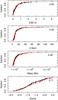 |
Fig. 1 Cumulative distributions of reddening, distance, stellar mass, and metallicity for GGCs in the top to bottom panels, respectively. Black curves represent the total sample (157 clusters) from the catalogue of Harris (1996, 2010 edition), and red curves are the sample from this work (51 clusters). The numbers in the panels are the p-values obtained by applying the Kolmogorov-Smirnov test to the black and red curves. |
Half of the targets were selected from the globular clusters catalogued by Harris (1996, 2010 edition)2 that are more distant and/or highly reddened; many of them are poorly studied.
The other half of the sample consists of well-known brighter objects, observed for
comparison with high-resolution spectroscopic studies available in the literature. In Fig.
1 we show the cumulative distribution of our sample
of 51 clusters in comparison with the total sample from the catalogue of Harris (1996, 2010 edition), in terms of reddening,
distance, stellar mass, and metallicity. Masses were calculated by Norris et al. (2014). When not available we estimated masses from the
MV −
M∗ relation (Eq. (1)) that we fitted from the Norris et al. (2014) data and applied to MV from Harris (1996, 2010 edition):  (1)The shapes of the distributions are very
similar. For an objective comparison, we ran Kolmogorov-Smirnov tests and all
p-values are
greater than 5%, meaning that the distributions are probably drawn from the same underlying
population. In other words, our sample is a bias-free representation of the Milky Way
globular cluster system.
(1)The shapes of the distributions are very
similar. For an objective comparison, we ran Kolmogorov-Smirnov tests and all
p-values are
greater than 5%, meaning that the distributions are probably drawn from the same underlying
population. In other words, our sample is a bias-free representation of the Milky Way
globular cluster system.
 |
Fig. 2 Sky positions of the 51 clusters studied in this work over a Milky Way image (Mellinger 2009) in terms of Galactic coordinates in an Aitoff projection. At the position of each cluster, a letter indicates its Galactic component, namely (B)ulge, (D)isc, (I)nner halo, and (O)uter halo, as given in Table A.1. |
The sample clusters were subdivided into the four Galactic components (bulge, disc, inner halo, and outer halo) following the criteria discussed by Carretta et al. (2010), except for bulge clusters that were classified in more detail by Bica et al. (2016), where a selection by angular distances below 20° of the Galactic center, galactocentric distances RGC ≤ 3.0 kpc, and [Fe/H] >−1.5 was found to best isolate bona fide bulge clusters. According to Carretta et al., outer halo clusters have RGC ≥ 15.0 kpc; the other objects are classified as disc or inner halo depending on their kinematics (dispersion or rotation dominated) and vertical distance with respect to the Galactic plane (see Carretta et al. 2010, for further details). The classification we adopted for each cluster is explicitly shown in Table A.1 together with the classifications of Carretta et al. and Bica et al. We assigned the clusters classified as non-bulge by Bica et al. to the disc cluster category, except for Pal 11, which is classified as inner halo by Carretta et al. The sky positions of our sample of clusters, categorized by Galactic component, are displayed over an all-sky image3 in Fig. 2.
Figure 3 shows reddening versus distance for our clusters in the bulge, disc, inner, and outer halo subsamples. The bulge clusters are located at similar distances from the Sun (~8 kpc) and are spread over a wide range of reddening values between ~0.2 and 1.5 depending on the direction. The closest disc clusters to the Sun have distances of ~2.3 kpc and the farthest are ~19 kpc from the Sun. Because of this distribution and the low latitudes of these clusters, reddening values vary from ~0.04 to ~1.7. The inner halo objects have similar intervals of E(B − V) and distance to the disc clusters. Outer halo clusters have low reddening, E(B − V) < 0.2 and are far from the Sun (11 < d(kpc) < 77).
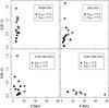 |
Fig. 3 Reddening versus distance of the 51 Milky Way globular clusters in our sample separated by Galactic component: bulge, disc, inner halo, and outer halo. Empty circles represent clusters with horizontal branch magnitude fainter than V = 17.5, filled circles are clusters with VHB brighter than 17.5. |
Identifications, coordinates, instrumental magnitudes and colours, and heliocentric radial velocities for all the stars observed.
To have homogeneous observations for all targets we chose the multi-object spectrograph, the FORS2 instrument on board the ESO Very Large Telescope (FORS2 at VLT/ESO; Appenzeller et al. 1998). This instrument enables observations of the faintest and brightest stars in our sample with a good compromise between S/N and exposure time. For example, the faintest stars we observed have V ≈ 19, and one hour of exposure with FORS24 results in S/N ~ 50 at this magnitude, which is sufficient for our techniques. Higher resolution spectrographs such as the FLAMES instrument on board the ESO Very Large Telescope (FLAMES at VLT/ESO) require prohibitive amounts of telescope time for stars of this faint magnitude. Specifically, the FLAMES user manual5 indicates that observations of stars with V = 17.5 with one hour of exposure will produce spectra with S/N ~ 30 using GIRAFFE fibres and S/N ~ 10 using UVES fibres. Stars fainter than that would require too much telescope time to obtain useful spectra. Consequently, detailed abundance studies based on optical spectra of stars in the more distant/reddened clusters are not feasible at the present time, and must await future Extremely Large Telescope (ELT) class facilities.
We selected red giant stars usually brighter than the horizontal branch level (see Paper I) in each cluster; therefore, the classification of globular clusters with VHB> 17.5 indicates which clusters could not be observed with high-resolution optical spectroscopy with current facilities. In Fig. 3 we note that half of the sample clusters (25 of 51) across all Galactic components are not bright enough for high-resolution observations. Thus, our survey represents a significant improvement in our knowledge of the chemical content of Milky Way globular clusters. We also note that 13 of the brightest clusters are in common with observations that defined the metallicity scale of Carretta et al. (2009a). In Sect. 4 we compare in more detail our results with previous metallicity scales.
Around 16 red giant stars were selected from photometry for each cluster from the pre-imaging observations for a total of 819 stars. We obtained FORS2 at VLT/ESO spectra for them, and 61 spectra (7%) were not considered in the analysis owing to very low S/N or data reduction problems. From the remaining 758 useful spectra, 465 (61%) are of confirmed member stars of the 51 clusters. The spectra were observed in the visible region (grism 1400V, 456–586 nm) with resolution of Δλ = 2.5 Å and typical S/N ~ 30−100. The data were collected from 2001 to 2012 under projects ID 68.B-0482(A, 2001), ID 69.D-0455(A, 2002), ID 71.D-0219(A, 2003), ID 077.D-0775(A, 2006), and ID 089.D-0493(B, 2012). Table A.1 lists the selected clusters, their coordinates, observing dates, and exposure times. Coordinates of the 758 analysed stars and their magnitudes are given in Table 1. The spectra were reduced using FORS2 pipeline inside the EsoRex software6 following the procedure described in Paper I.
3. Method
The method for atmospheric parameter derivation was described and exhaustively discussed in Paper I, and can be summarized as follows. Atmospheric parameters (Teff, log(g), [Fe/H], [Mg/Fe], [α/Fe]) were derived for each star by applying full spectrum fitting through the code ETOILE (Katz et al. 2011 and Katz 2001). The code takes into account a priori Teff and log(g) intervals for red giant branch (RGB) stars and carries out a χ2 pixel-by-pixel fitting of a given target spectrum to a set of template spectra. We chose two libraries of template stellar spectra, one empirical (MILES, Sánchez-Blázquez et al. 2006) and one synthetic (Coelho et al. 2005, hereafter referred to as Coelho).
The library spectra are sorted by similarity (S, proportional to χ2, see Paper I) to the target spectrum and the parameters are calculated by taking the average of the parameters of the top N template spectra. For the Coelho library we adopted N = 10, and for the MILES library N is defined such that S(N) /S(1) ≲ 1.1. For each star, [Mg/Fe] is given by the MILES templates only; [α/Fe] is given by the Coelho templates only; and Teff, log(g), and [Fe/H] are the averages of the MILES and Coelho results. Uncertainties of Teff, log(g), [Fe/H], [Mg/Fe], and [α/Fe] for each star are the standard deviation of the average of the top N templates. It is difficult to estimate the correlation between the parameters because of the nature of the adopted analysis technique (see details in Paper I). The uncertainties of the average of the MILES and Coelho results for each star are calculated through conventional propagation, as are the uncertainties for the average [Fe/H] for the member stars of each globular cluster.
We note that before running the comparison of a given target spectrum with the reference spectra, two important steps are needed: convolving all the library spectra to the same resolution of the target spectrum, and correcting them for radial velocities, also measured with the same ETOILE code using a cross-correlation method with one template spectrum. For detailed discussion of this method and validation with well-known stars and high-resolution analysis, we refer to Paper I.
Membership selection of stars for each cluster was done in two steps: first, by radial velocities and metallicities; second, by proximity of temperature and surface gravity to reference isochrones, which is independent of reddening. In this way we use all the derived atmospheric parameters as input in the selection of member stars. Examples and a detailed description are given in Paper I.
4. Results and comparison with previous metallicity scales
Atmospheric parameters for all 758 studied stars are presented in Table A.2 following the IDs from Table 1. We list Teff, log(g), and [Fe/H] from both the MILES and Coelho libraries, and the averages of these values are adopted as our final parameters (see Paper I for a detailed justification of this procedure). Table A.2 also lists [Mg/Fe] from MILES and [α/Fe] from the Coelho library. The average of [ Fe / H ], [ Mg / Fe ], [ α/ Fe ], and vhelio for the 51 clusters based on their selected member stars are presented in Table A.3. Metallicities from the MILES and Coelho libraries are given; the average of these results is our final abundance for the clusters. We note that while there are some clusters that are known to possess sizeable spreads in individual [Mg/Fe] values, as a result of the light element chemical anomalies usually referred to as the O-Na anti-correlation, in most cases the spread in [Mg/Fe] is small (e.g. Carretta et al. 2009b; Fig. 6). Therefore, our approach of averaging all the determinations for a given cluster should not substantially bias the mean value.
The previous largest abundance collection for GGCs was done by Pritzl et al. (2005) for 45 objects, containing [Fe/H], [Mg/Fe], [Si/Fe], [Ca/Fe], [Ti/Fe], [Y/Fe], [Ba/Fe], [La/Fe], and [Eu/Fe]. More recently Roediger et al. (2014) has compiled chemical abundances from the literature for 41 globular clusters, including [Fe/H], [Mg/Fe], [C/Fe], [N/Fe], [Ca/Fe], [O/Fe], [Na/Fe], [Si/Fe], [Cr/Fe], and [Ti/Fe]. The caveats of these compilations are that they are based on heterogeneous data available in the literature, and the objects are mostly halo clusters for the Pritzl et al. sample. Our results represent the first time that [Fe/H], [Mg/Fe], and [α/Fe], derived in a consistent way, are given for such a large sample of globular clusters (51 objects); this number is almost one-third of the total number of catalogued clusters (157 as compiled by Harris 1996, 2010 edition), and includes all Milky Way components.
In the following sections we compare our metallicity determinations with five other works that report homogenous metallicities for at least 16 GGCs. We begin with the high-resolution study of (Carretta et al. 2009a, hereafter C09) described in Table 3.
4.1. Carretta et al. (2009a) scale
Carretta et al. (2009a) reported a new metallicity scale for Milky Way globular clusters based on their observations of 19 clusters with UVES (Carretta et al. 2009b) and GIRAFFE (Carretta et al. 2009c) at VLT/ESO. This scale superseded their previous scale (Carretta & Gratton 1997). In our survey there are 13 objects in common with their sample covering the metallicity range −2.3 < [ Fe / H ] < −0.4, as shown in Table 2. Carretta et al. added two metal-rich clusters, NGC 6553 and NGC 6528, with previous high-resolution spectroscopy to increase the metallicity range up to solar abundance; specifically, they adopted the abundances from Carretta et al. (2001) who showed that these clusters have similar metallicities, and that NGC 6528 is slightly more metal-rich. They derived [Fe/H] = + 0.07 ± 0.10 for NGC 6528 and then offset the value [Fe/H] = −0.16 ± 0.08 for NGC 6553 from Cohen et al. (1999, C99) to [Fe/H] = −0.06 ± 0.15, a value closer to the one they found for NGC 6528. However, the metallicity derived by C99 agrees well with more recent work. For example, Meléndez et al. (2003, M03) and Alves-Brito et al. (2006, AB06) derived [Fe/H] = −0.2 ± 0.1 and [Fe/H] = −0.20 ± 0.02 for this cluster. Therefore, the original value of C99 for NGC 6553 should be retained. We adopt here the weighted mean metallicity of C99, M03, and AB06 for NGC 6553. In the case of NGC 6528 a more recent work derived [Fe/H] = −0.1 ± 0.2 (Zoccali et al. 2004, Z04), and we took the weighted mean metallicity of the values from Z04 and C01 as our reference for NGC 6528. All values are compiled in Table 2.
Average [Fe/H] from this work compared with the 13 globular clusters in common with C09.
Our [Fe/H] results are compared with the 13 clusters from C09 plus the two metal-rich
clusters (see Table 2) averaged from other sources
in Fig. 4 where the cluster names are indicated. The
metal-rich clusters are indicated by circles and they are included in the linear fit of
Eq. (2), represented by the blue line in
the plot, and valid in the metallicity range −2.4 < [ Fe / H ] < 0.0:![\begin{equation} {\rm [Fe/H]}_{\rm C09} = -0.05(\pm0.04) + 0.99(\pm0.03){\rm [Fe/H]}_{\rm FORS2} \label{eq:fesh-car09} . \end{equation}](/articles/aa/full_html/2016/06/aa26765-15/aa26765-15-eq59.png) (2)Metallicities of the two metal-rich clusters
adopted by Carretta et al. (2001) are overplotted as
red circles in Fig. 4 for reference, but they are not
included in the fit.
(2)Metallicities of the two metal-rich clusters
adopted by Carretta et al. (2001) are overplotted as
red circles in Fig. 4 for reference, but they are not
included in the fit.
 |
Fig. 4 Comparison of [Fe/H] from this work with those from C09 for the 13 clusters in common plus NGC 6553 from C01 and Z04, and NGC 6528 from C99, M03, and AB06. The black line is the one-to-one relation and the blue line is the linear fit to the 15 black points (Eq. (2)). Residuals are presented in the bottom panels. The blue dashed lines represent ± 1σ. Metallicities adopted by Carretta et al. (2001) are shown in red for reference, but they are not considered in the fit. Values are listed in Table 2. |
From Eq. (2) we can conclude that our metallicity results are in excellent agreement with those from high-resolution spectroscopy because the slope of the fit is compatible with 1.0 and the offset is near zero. The correlation coefficient, r2 = 0.99, is close to unity and there is no indication of any correlation between the residuals and metallicity, which justifies the use of a linear relation. The standard deviation, σ = 0.08 dex, can be explained by the uncertainties in the individual cluster metallicities (see Table 2, where our abundances are an excerpt of Table A.3). Moreover, the residuals plot shows explicitly that the [Fe/H] values adopted by Carretta et al. (2001) for NGC 6528 and NGC 6553 are shifted upwards from the relation by at least 1σ with respect to our adopted values. The consistency of our results with C09 (complemented by metal-rich clusters from other works based on high-resolution spectroscopy) scale in the entire range −2.4< [Fe/H] < 0.0 and supports the robustness of the metallicities derived from full spectrum fitting of low- or medium-resolution spectroscopy.
We also note that C09 used their adopted metallicities for NGC 6553 and NGC 6528 in their recalibration of other metallicity scales. Since we have adopted lower metallicities for these clusters, values that agree well with other high-resolution spectroscopic work, the calibration of other metallicity scales – particularly for the metal-rich tail – needs to be reconsidered.
4.2. Zinn and West scale
Zinn & West (1984) published a metallicity
scale 30 years ago that is still a reference, although it is based on the integrated-light
index Q39 (Zinn
1980). We compare their Q39 index with our final [Fe/H] values
for the 31 clusters in common in Fig. 5. The relation
is described well by the second-order polynomial of Eq. (3): ![\begin{equation} \begin{array}{@{}ll} {\rm [Fe/H]}_{\rm FORS2} =&\!\!\!\! -1.92(\pm 0.05) + 5.6(\pm 0.6)\cdot Q_{39} \\[1mm] &\!\!\!\!-4.2(\pm 1.4)\cdot Q_{39}^2. \end{array} \label{eq:q39-d14} \end{equation}](/articles/aa/full_html/2016/06/aa26765-15/aa26765-15-eq64.png) (3)The fitting quality parameters are
r2 =
0.93 and σ
= 0.18 dex for the interval −2.44 < [ Fe / H ] < −0.08. Figure 5 shows the data points with Eq. (3) plotted in the blue solid line, while the red dashed line represents the
curve fitted by C09 against their UVES metallicities. Both curves agree well for [Fe/H]
≲−0.4, but there is a small divergence for
the most metal-rich clusters. The C09 red curve has higher metallicities for the most
metal-rich clusters because they adopted the higher metallicities for NGC 6528 and NGC
6553 from Carretta et al. (2001), as discussed in
the previous section.
(3)The fitting quality parameters are
r2 =
0.93 and σ
= 0.18 dex for the interval −2.44 < [ Fe / H ] < −0.08. Figure 5 shows the data points with Eq. (3) plotted in the blue solid line, while the red dashed line represents the
curve fitted by C09 against their UVES metallicities. Both curves agree well for [Fe/H]
≲−0.4, but there is a small divergence for
the most metal-rich clusters. The C09 red curve has higher metallicities for the most
metal-rich clusters because they adopted the higher metallicities for NGC 6528 and NGC
6553 from Carretta et al. (2001), as discussed in
the previous section.
 |
Fig. 5 Q39 index from Zinn (1980) against [Fe/H] from this work. The blue solid line is the quadratic function fitted to the data (Eq. (3)) and the red dashed line is the quadratic function fitted by C09 to calibrate Q39 to their scale. Fitted curves are shown only in their respective valid ranges. |
4.3. Rutledge scale
Rutledge et al. (1997) published a metallicity
scale based on the reduced equivalent widths (W′) of the near infrared CaII triplet lines for 52
clusters. We have 18 clusters in common and the best-fit quadratic function relating their
W′ values
to our [Fe/H] determinations is given by ![\begin{equation} \begin{array}{@{}ll} {\rm [Fe/H]}_{\rm FORS2} =&\!\!\!\! -2.65(\pm 0.28) + 0.13(\pm 0.17)\cdot \langle W'_{\rm R97}\rangle \\[2mm] &\!\!\!\! + 0.067(\pm 0.025)\cdot \langle W'_{\rm R97}\rangle ^2. \end{array} \label{eq:r97-d14} \end{equation}](/articles/aa/full_html/2016/06/aa26765-15/aa26765-15-eq71.png) (4)The fit parameters are r2 = 0.97 and
σ = 0.13
dex for the interval −2.27<
[Fe/H] <−0.08. Figure 6 displays the fitted curve as the blue solid line, while the cubic function
fitted by C09 is shown as the dashed line. As in the case of Zinn & West scale, Fig.
6 shows that our curve agrees well with that of
C09, with a slight discrepancy for clusters with [Fe/H] ≳−0.4, where the C09 relation gives higher metallicities for the
metal-rich clusters. The origin of this difference is as discussed above.
(4)The fit parameters are r2 = 0.97 and
σ = 0.13
dex for the interval −2.27<
[Fe/H] <−0.08. Figure 6 displays the fitted curve as the blue solid line, while the cubic function
fitted by C09 is shown as the dashed line. As in the case of Zinn & West scale, Fig.
6 shows that our curve agrees well with that of
C09, with a slight discrepancy for clusters with [Fe/H] ≳−0.4, where the C09 relation gives higher metallicities for the
metal-rich clusters. The origin of this difference is as discussed above.
 |
Fig. 6 Reduced equivalent width ⟨ W′ ⟩ from CaII triplet from Rutledge et al. (1997) against [Fe/H] from this work. The blue solid line is the quadratic function fitted to the data (Eq. (4)) and the red dashed line is the cubic function fitted by C09 to calibrate ⟨ W′ ⟩ R97 to their scale. Fitted curves are shown only in their respective valid ranges. |
4.4. Kraft and Ivans scale
Kraft & Ivans (2003) collected a
non-homogeneous set of high-resolution stellar spectra of 16 clusters with [Fe/H]
<−0.7 and proceeded with a homogeneous
analysis. We have ten clusters in common with the Kraft & Ivans abundances related to
ours by the linear function given in Eq. (5): ![\begin{equation} \begin{array}{@{}l} {\rm [Fe/H]}_{\rm FORS2} = -0.16(\pm 0.12) + 0.94(\pm 0.08)\cdot {\rm [Fe/H]_{KI03}}. \end{array} \label{eq:ki03-d14} \end{equation}](/articles/aa/full_html/2016/06/aa26765-15/aa26765-15-eq78.png) (5)The fit parameters are r2 = 0.94 and
σ = 0.11
dex for the interval −2.28<
[Fe/H] <−0.66. Our relation, the blue line in Fig.
7, and that of C09, the red dashed line in the same
figure, are essentially identical to the Kraft & Ivans sample, which lacks clusters
more metal-rich than [Fe/H] >−0.7
(Kraft & Ivans 2003).
(5)The fit parameters are r2 = 0.94 and
σ = 0.11
dex for the interval −2.28<
[Fe/H] <−0.66. Our relation, the blue line in Fig.
7, and that of C09, the red dashed line in the same
figure, are essentially identical to the Kraft & Ivans sample, which lacks clusters
more metal-rich than [Fe/H] >−0.7
(Kraft & Ivans 2003).
4.5. Saviane scale
Saviane et al. (2012a) analysed spectra from
FORS2/VLT obtained in the same project as the data presented here, but they analysed the
CaII triplet lines in a similar way to Rutledge et al.
(1997). Saviane et al. (2012a) studied a
total of 34 clusters, of which 14 were used as calibration clusters, and the other 20 were
programme clusters. There are 27 clusters in common and Eq. (6) shows the quadratic relation between the
 values and our metallicities. The fit
parameters are r2 = 0.97 and σ = 0.12 dex for the
interval −2.28< [Fe/H] <−0.08:
values and our metallicities. The fit
parameters are r2 = 0.97 and σ = 0.12 dex for the
interval −2.28< [Fe/H] <−0.08: ![\begin{equation} \begin{array}{@{}ll} {\rm [Fe/H]}_{\rm FORS2} =&\!\!\!\! -2.55(\pm 0.25) + 0.03(\pm 0.14)\cdot \langle W'_{\rm S12} \rangle \\[2mm] &\!\!\!\! + 0.068(\pm 0.018)\cdot \langle W'_{\rm S12} \rangle ^2. \end{array} \label{eq:s12-d14} \end{equation}](/articles/aa/full_html/2016/06/aa26765-15/aa26765-15-eq82.png) (6)Figure 8
shows the fit as the blue solid line while the red dashed curve shows the calibration
relation adopted by Saviane et al. (2012a), which
uses the metallicities from C09 as reference values. Saviane et al. (2012a) used metal-poor stars ([Fe/H] <−2.5) to conclude that their
metallicity–line strength relation cannot be extrapolated, i.e. it is only valid in the
interval from
(6)Figure 8
shows the fit as the blue solid line while the red dashed curve shows the calibration
relation adopted by Saviane et al. (2012a), which
uses the metallicities from C09 as reference values. Saviane et al. (2012a) used metal-poor stars ([Fe/H] <−2.5) to conclude that their
metallicity–line strength relation cannot be extrapolated, i.e. it is only valid in the
interval from  = 1.69 to
 . The excellent agreement between the
curves in Fig. 8 allows us to conclude that CaII
triplet metallicities from FORS2/VLT spectra can be calibrated using metallicities for the
same objects derived from visible spectra observed with the same instrument.
. The excellent agreement between the
curves in Fig. 8 allows us to conclude that CaII
triplet metallicities from FORS2/VLT spectra can be calibrated using metallicities for the
same objects derived from visible spectra observed with the same instrument.
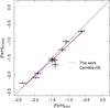 |
Fig. 7 [Fe/H] from Kraft & Ivans (2003) against [Fe/H] from this work. The blue solid line is the linear function fitted to the data (Eq. (5)) and the red dashed line is the linear function fitted by C09 to calibrate [Fe/H]KI03 to their scale. Fitted curves are shown only in their respective valid ranges. |
 |
Fig. 8 Reduced equivalent width ⟨ W′ ⟩ from CaII triplet from Saviane et al. (2012a) against calibrated [Fe/H] from this work. The blue solid line is the quadratic function fitted to the data (Eq. (6)) and the red dashed line is the cubic function fitted by Saviane et al. (2012a) to calibrate their ⟨ W′ ⟩ S12 to the Carretta scale. Fitted curves are shown only in their respective valid ranges. |
Summary of the properties of the current and previous metallicity scales.
4.6. Conclusions on metallicity scales
The information discussed in the preceding sections is compiled in Table 3. The metallicity range is roughly the same for all the scales with exception of the Kraft & Ivans (2003) scale, which does not have clusters more metal-rich than [Fe/H] ≳−0.5. The largest homogeneous sample is still that of Zinn & West (1984), but their study is based on integrated light which brings in a number of difficulties as discussed in the Zinn & West (1984) paper. All the other data sets are based on measurements for individual stars. The largest homogeneous sample is then that of Rutledge et al. (1997). However, it is based on a CaII triplet index which requires calibration to a [Fe/H] scale. C09 is the largest sample based on high-resolution spectroscopy, although it has only 19 clusters with no cluster having [Fe/H] >−0.4. Our results from R ~ 2000 stellar spectra cover the entire metallicity range of −2.4< [Fe/H] < 0.0, and they are shown above to be compatible with the high-resolution metallicities from C09, complemented by metal-rich clusters from other high-resolution spectroscopic studies.
C09 calibrated all previous metallicity scales to theirs and averaged them in order to get the best metallicity estimate for all catalogued clusters. In Fig. 9 we compare these values to those derived here for the Milky Way clusters in our FORS2 survey (see Table A.3). There are 45 clusters in common. A one-to-one line is plotted to guide the eye. The [Fe/H] values are in good agreement with the residuals shown in the bottom panel and reveal no trends with abundance. The 15 clusters used to compare our [Fe/H] determinations to the C09 scale (cf. Sect. 4.1) are highlighted as red triangles. The dispersion of the residuals is σ = 0.16 dex, which is of the order of the dispersion of the fit of all previous metallicity scales to ours (Table 3). If C09 had averaged the metallicity scales without having calibrating them to their scale, this dispersion would be higher. Furthermore, the residuals do not show trends with abundance, which supports the agreement of our results with C09 as discussed in Sect. 4.1. Consequently, our metallicities are sufficiently robust to be used as references, from the most metal-poor to solar-metallicity Milky Way globular clusters with a precision of ~0.1 dex. Moreover our data complement the existing spectroscopic information on the Galactic GC system by reducing the existing bias in the GC data base against distant and reddened clusters.
 |
Fig. 9 Comparison of the [Fe/H] values from this work with those from C09 for the 45 clusters of our survey using values of Table A.3. Red triangles emphasize the 15 clusters used to compare with C09 in Sect. 4.1. Blue points are the six clusters not averaged by Carretta et al. (2009a) and analysed for the first time in a homogenous way in this work. A one-to-one line is plotted for reference. The residuals of the comparison are displayed in the bottom panel and have a standard deviation equal to 0.16 dex. |
We have also shown that CaII triplet indices based on spectra from the same instrumentation set-up can be calibrated using our [Fe/H] values, or C09’s, producing very similar results. Moreover this work also provides the largest sample of homogeneous [Mg/Fe] and [α/Fe] values for Milky Way globular clusters. In addition, six clusters not contained in Carretta et al. (2009a) have their metallicities determined from individual star spectra and a homogenous analysis for the first time. The clusters are BH 176, Djorg 2, Pal 10, NGC 6426, Lynga 7, and Terzan 8 and they are shown as blue points in Fig. 9. Moreover, the first three clusters only had photometric metallicities estimations until now, and the available metallicity for NGC 6426 came from integrated spectroscopy and photometry only.
5. Chemical evolution of the Milky Way
The ratio [α/Fe] plotted against [Fe/H] provides an indication of the star formation efficiency in the early Galaxy. Nucleosynthetic products from type II supernovae (SNII) are effectively ejected shortly after the formation of the progenitor massive star, releasing predominantly α-elements together with some iron7 into the interstellar medium. Type Ia supernovae (SNIa) of a given population, on the other hand, start to become important from 0.3 Gyr to 3 Gyr after the SNII events, depending on the galaxy properties (Greggio 2005). These SN generate most of the Fe in the Galaxy, decreasing the [α/Fe] ratio. Magnesium is one of the α-elements and represents these processes well. Increasing values of [Fe/H] indicate subsequent generations of stars so that lower metallicities and higher [α/Fe] stand for first stars enriched by SNII and higher metallicities and lower [α/Fe] stand for younger objects enriched by SNIa. The location of the turnover, designated by [Fe/H]knee, identifies when SNIa start to become important.
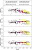 |
Fig. 10 [Mg/Fe] and [α/Fe] for the 51 clusters from this work in comparison with disc and halo field stars from Venn et al. (2004), bulge field stars from Gonzalez et al. (2011), and clusters from Pritzl et al. (2005). In the panels with [Ti/Fe], [⟨Ca,Ti⟩/Fe], and [⟨Mg,Ca,Ti⟩/Fe], our results are [α/Fe] (see text for details). |
Figure 10 displays the distribution along [Fe/H] of [Mg/Fe], [Ti/Fe], two alternatives to represent the average [α/Fe] (i.e. [⟨Ca, Ti⟩/Fe] and [⟨Mg, Ca, Ti⟩/Fe]) for halo and disc field stars from Venn et al. (2004), bulge field stars from Gonzalez et al. (2011), and clusters from Pritzl et al. (2005). We overplot our results on [Mg/Fe] versus [Fe/H] in the uppermost panel, and [α/Fe] versus [Fe/H] in the other three panels for the 51 globular clusters in our sample. The dispersion of our points is smaller than that of the Pritzl et al. points in all the panels. We note that our results were derived from homogeneous observations and analysis of R ~ 2000 spectra, while those from Pritzl et al. come from a compilation of different works based on higher resolution spectroscopy from the literature.
Whether globular clusters should follow the same pattern as field populations or not is an open question. Qualitative analysis of the metal-poor region of the panels in Fig. 10 with [Fe/H] <−1.0 shows that our results for [Mg/Fe] agree well with the Pritzl et al. clusters and also with disc+halo stars. Our results for [α/Fe] reveal a positive slope, which leads to lower values with respect to [Ti/Fe], [⟨Ca, Ti⟩/Fe], and [⟨Mg, Ca, Ti⟩/Fe] for disc+halo stars. Nevertheless, the Pritzl et al. results also present a positive slope for [Ti/Fe] distribution, despite their large dispersion. It appears that our results for [α/Fe] are closer to those from Pritzl et al. for [Ti/Fe] than to the average of alpha-element enhancements.
Pritzl et al. do not have many clusters in the metal-rich regime where [Fe/H] >−1.0 bulge stars clearly split from disc+halo stars and the [Fe/H]knee is less obvious than that in the [Mg/Fe] panel; therefore, any comparison with their results would be poor. Our distribution of [Mg/Fe] follows that of disc+halo stars, while our [α/Fe] is as enhanced as that for bulge stars.
Pritzl et al. (2005) found a few peculiar cases. Some of these are in common with our FORS2 survey data: two metal-rich bulge clusters, NGC 6553 and NGC 6528, and the metal-poor [α/Fe]-depleted halo cluster, Rup 106. We indicate these clusters explicitly in Fig. 10; in particular, the lower three panels with [α/Fe] confirm that Rup 106 has a lower [α/Fe] ratio than the other clusters and also lower than halo and disc stars at similar metallicities. The bulge clusters NGC 6553 and NGC 6528 follow the bulge stars. We have shown in Paper I that our abundances of [α/Fe] for NGC 6528 and NGC 6553 are in agreement with high-resolution spectroscopic results. We were able to recover a subtle depletion in [α/Fe] for Rup 106 and an enhancement in [α/Fe] for NGC 6528 and NGC 6553.
We note that our [α/Fe] is derived from the comparison with the Coelho library; here the spectra are modelled by varying all α-elements O, Mg, S, Si, Ca, and Ti. The [α/Fe] distribution matches that of [Ti/Fe] better than other elements and does not show the turnover. It is interesting to note that in the metal-rich regime, Lecureur et al. (2007) found enhancements of Na and Al; therefore, the metal-rich bulge stars might show other unexpected behaviour. Further checks are underway that vary each element individually, rather than varying all alpha-elements together as is done in Coelho et al. (2005). The analysis approach could be improved in the future by including stars from the Magellanic Clouds, which generally have lower [α/Fe] than the Galaxy at higher metallicities (e.g. Van der Swaelmen et al. 2013).
6. Horizontal branch morphology and the second parameter problem
 |
Fig. 11 Metallicity as a function of horizontal branch morphology (HB index) for all 51 clusters of our sample, where HB index is from Mackey & van den Bergh (2005). Three isochrones from Rey et al. (2001) are overplotted, where t0 is the mean age of inner halo clusters as defined by Rey et al. as RGC< 8 kpc. Ages from VandenBerg et al. (2013) are available only for 17 out of 51 clusters in our sample, and are shown as red, purple, and blue circles for young, intermediate-age, and old clusters. The hatched triangle shows the region of the Oosterhoff gap as defined by Catelan (2009). |
The horizontal branch (HB) morphology in a colour magnitude diagram (CMD) of a globular cluster is shaped mainly by metallicity, but there are other parameters that influence its predominant colour. These include age, helium abundance, CNO abundance, and RGB mass-loss, among others (see review of Catelan 2009 and references therein). All phenomena may be shaping the HB together, with one more important than the others; for example, the second parameter is traditionally assumed to be age, but there are exceptions (e.g. Fusi Pecci & Bellazzini 1997). Figure 11 shows the effect of age (from VandenBerg et al. 2013 when available) and metallicity (from this work) on the colour of the horizontal branch, with the HB index being (B − R) / (B + V + R), where B, R, and V are the number of blue, red, and variable stars (Lee et al. 1994). The older or more metal-poor the cluster, the bluer the HB; redder HB represents younger and/or more metal-rich clusters. Three HB isochrones with different ages from Rey et al. (2001) are shown.
We call attention to four groups of clusters in the plot, all of them indicated in Fig. 11:
-
NGC 2808: typical bimodal HB (e.g. Corwin et al. 2004).
-
M 68, NGC 6426, and M 15: M 68 possibly has age as the second parameter (VandenBerg et al. 2013). NGC 6426 is older, contrary to what is expected from Fig. 11 (Hatzidimitriou et al. 1999). M 15 is one of the two clusters (of 16) that do not follow the blue HB distribution of field stars (Brown et al. 2005).
-
M 10, NGC 6752, and NGC 6749: the first has a HB morphology possibly justified by He variations (Gratton et al. 2010). The second has a very complex HB morphology (Momany et al. 2002). The third cluster has a CMD from Rosino et al. (1997) and no discussion on the second parameter problem.
-
HP 1, NGC 6558, and NGC 6284: the first two have been studied by (Ortolani et al. 1997, 2011; Barbuy et al. 2006, 2007) and are candidates for the oldest clusters in the bulge. The third has a CMD from HST observations and no discussion about HB morphology (Piotto et al. 2002).
The first three groups have been well discussed in the literature, with the exception of NGC 6749, which should be analysed in more detail. For a review on the topic we refer to Catelan (2009) and Gratton et al. (2010). To look for the oldest clusters in the Milky Way, we focus the discussion of the last group as follows.
For this group of clusters with blue HB and [Fe/H] ~−1.0, there are some possible explanations: (i) the clusters are older than all others; (ii) their He abundance is lower; or (iii) their CNO abundance is lower. Figure 11 can only reveal if age and metallicity are able to explain the HB morphology. Fixing the HB index and [Fe/H] and varying only age, these clusters would be the oldest objects in the Milky Way by projecting the age gradient from the isochrones upwards in the plot. As a result, deriving ages and HB star abundances for these clusters is crucial to make such strong conclusion. VandenBerg et al. (2013) have not published ages for these clusters, but other papers have, as is discussed below.
NGC 6284
This is a disc cluster located behind the bulge with E(B − V) = 0.28, 7.5 kpc from the Galactic centre and out of the projected plane of the X-shaped bulge. This location likely rules out the possibility of NGC 6284 being a bulge cluster ejected by the dynamics of the “X”. Catelan (2009) noticed some peculiarities about NGC 6284 and classified it as an Oosterhoff-intermediate globular cluster, yet it does not fall in the region (indicated by a triangle in Fig. 11) where such clusters are expected. Piotto et al. (2002) presented a HST-based CMD showing a clear blue HB, therefore its index is verified. We derived a metallicity of [Fe/H] = −1.07 ± 0.06 for this cluster which is more metal-rich yet still compatible to within 2.2σ with the value of −1.31 ± 0.09 (Q39 index from Zinn 1980 calibrated to the scale presented by Carretta et al. 2009a). Meissner & Weiss (2006) derived 11.00 ± 0.25 Gyr8 for NGC 6284, which is relatively young for a globular cluster and may rule out the proposition that NGC 6284 could be among the oldest objects in the Milky Way. For this cluster, even if age is helping to shape the blue HB, a lower He and/or CNO abundance should be important factors.
HP 1
This bulge cluster is the innermost globular cluster known in the Milky Way, with E(B − V) = 1.12 and only 500 pc from the Galactic centre where Sgr A* with the central black hole and surrounding nuclear star cluster are located (Genzel et al. 2010). The contamination of foreground and background stars and dust is very high, and Ortolani et al. (2011) performed a decontamination using proper motion with a baseline of 14 years. Even with Multi-Conjugate Adaptive Optics at the VLT (MAD/VLT) photometry producing a well-defined CMD, it only reaches the subgiant branch and the main sequence turnoff is undersampled. With this information they estimated an age of 13.7 Gyr relative to other well-studied clusters. The respective isochrone (assuming Z = 0.002, [Fe/H] ≈−0.9) agrees well with the current CMD. A lower limit for the age for HP 1 based on their method would be 12.7 Gyr. This result supports the prediction of an old age from Figure 11. We derived [Fe/H] = −1.17 ± 0.07 from the average of eight red giant stars in the cluster, which is compatible with [Fe/H] = −1.0 ± 0.2 found by Barbuy et al. (2006) from the analysis of high-resolution UVES spectra of two red giant stars. They derived [Mg/Fe] = 0.10 and we found a more alpha-enhanced ratio comparable to bulge field stars of similar metallicity, [Mg/Fe] = 0.33 ± 0.07. We confirm that HP 1 is one of the top candidates for the oldest globular cluster in our Galaxy, sharing the age of the Milky Way. The orbit of HP 1 was derived by Ortolani et al. (2011) and Rossi et al. (in prep.), showing that it is confined within the bulge/bar. The central region was the densest environment of the proto-galaxy where globular clusters probably formed first. Deeper photometry is needed to better sample the main sequence turnoff and to have a definitive isochrone fitting, which makes it a perfect target for ACS/HST or the forthcoming E-ELT.
NGC 6558
This bulge cluster was extensively discussed in Paper I where we show the compatibility of our results with those of Barbuy et al. (2007), star by star. Therefore, we concentrate on further discussion about its role in this special group in the [Fe/H]-HB index plot. We also highlight the new abundance uncertainty using the updated criteria described in Sect. 3: [Fe/H] = −1.01 ± 0.05 and [Mg/Fe] = 0.26 ± 0.06. Barbuy et al. (2007) derived [Fe/H] = −0.97 ± 0.15 and [Mg/Fe] = 0.24, which are compatible with our results. The horizontal branch is very similar to that of HP 1 (Barbuy et al. 2007; Ortolani et al. 2011); therefore, the position of NGC 6558 in Fig. 11 is valid. The age of the cluster is a more difficult matter. Barbuy et al. (2007) have fitted two isochrones of 14 Gyr in a CMD containing cluster and field stars; Alonso-García et al. (2012) has shown a differential reddening varying from −0.06 to +0.08 with respect to the average E(B − V) = 0.44; and Rossi et al. (2015) have published a proper motion cleaned CMD which shows a broad RGB but with less deep photometry and an undersampled main sequence turnoff. These complexities may lead to uncertainties in the age derivation, but the spread of the main sequence turnoff is less than ΔV ≈ 0.2 mag, which would make it difficult to measure the relative age to better than 1 Gyr. We conclude that NGC 6558 should not be classified among the younger globular clusters. Consequently, it may be that age is a strong candidate for the second parameter in the case of this cluster causing a blue HB and placing it as one of the oldest objects in the Milky Way. As proposed for HP 1 above, high-resolution spectroscopy of HB stars is needed in order to understand the role of He and CNO and further constrain the age.
7. Summary and conclusions
In this work we present parameters – derived from R ~ 2000 visible spectra by applying the methods described in Paper I – for 51 GGCs. We observed 819 red giant stars and analysed 758 useful spectra; of these we classified 464 stars as members of the 51 clusters and 294 as non-members. Membership selection included deriving radial velocities for all 758 spectra. Estimates for Teff, log(g), and [Fe/H] were determined by using observed (MILES) and synthetic (Coelho) spectral libraries and the results from both libraries averaged for the final results. We compared our results with five previous metallicity scales and fit polynomial functions with coefficients of determination r2 ≥ 0.93 and σ ≤ 0.18 dex. The most important comparison is against C09, which contains the largest sample of clusters (19) with abundances based on high-resolution spectroscopy. For this case, a linear fit was very good with r2 = 0.99 and σ = 0.08 dex. The slope of the fit is compatible with 1.0 and the offset is near zero, which means that our metallicity results are in excellent agreement with those from high-resolution spectroscopy in the range −2.5≲ [Fe/H] ≲ 0.0 with no need to apply any scale or calibration. The other scales are based on lower resolution spectroscopy, CaII triplet, limited sample, or integrated light, and the functions fitted against our metallicities are compatible with those fitted against the C09 results, except for the metal-rich regime for which we used updated and robust references from high-resolution spectroscopy. Metal-rich clusters with [Fe/H] ≳−0.5 are less metal-rich than the findings of C09. An important consequence of our results is that CaII triplet line strengths, such as those of Saviane et al. (2012a), can be calibrated directly by applying our approach to visible region spectra of the same stars obtained with the same instrument.
C09 took an average of metallicities available at that time for all globular clusters from different metallicity scales after calibration to their scale. For the 45 clusters in common with our sample, the comparison has no trends with abundance and a dispersion of σ = 0.16 dex, in agreement with our comparison to the same metallicity scales. The metallicities derived in this work are robust to within 0.1 dex for the entire range of [Fe/H] shown by GGCs. Six clusters of our sample do not have previous measurements presented in Carretta’s scale. The clusters are BH 176, Djorg 2, Pal 10, NGC 6426, Lynga 7, and Terzan 8 and we present abundances for these clusters in a homogeneous scale for the first time. Moreover, the first three clusters have only had photometric metallicities estimations until now, and the available metallicity for NGC 6426 came only from integrated spectroscopy and photometry.
Another important product of this survey is that we also provide [Mg/Fe] and [α/Fe] for all 758 stars and the average values for member stars in the 51 clusters on a homogeneous scale. This is the largest sample of α-element abundances for Milky Way globular clusters using the same set-up for observations and same method of analysis. The distribution of [Mg/Fe] with [Fe/H] for the 51 clusters follows the same trends as for field stars from the halo and disc, but does not recover the peculiar α-element depletion for the metal-poor halo cluster Rup 106, and does not support high [α/Fe] for clusters like NGC 6553 and NGC 6528. The [α/Fe], [Fe/H] relation follows the trend of bulge stars, and recovers abundances for NGC 6553, NGC 6528 compatible with bulge field stars, as well as the depletion in [α/Fe] for Rup 106. However, the distributions of [Mg/Fe] and [α/Fe] with [Fe/H] do not agree well with each other possibly because [α/Fe] is derived from the comparison with the Coelho library, which models the spectra by varying all α-elements O, Mg, S, Si, Ca, and Ti, while for the clusters the observed [α/Fe] is the average of [Mg/Fe], [Ca/Fe], and [Ti/Fe] only. We intend to improve α-element abundance measurements in a future paper.
The metallicities derived in this work were plotted against the index of horizontal branch morphology and we identified four peculiar groups in the diagram. We then focused on the group containing the metal-rich and blue horizontal branch clusters HP 1, NGC 6558, and NGC 6284. These clusters are candidates for the oldest objects in the Milky Way. HP 1 and NGC 6558 possess bluer horizontal branch morphologies than expected for their metallicities of [Fe/H] = −1.17 ± 0.07 and −1.01 ± 0.05, respectively. If the second parameter that drives the morphology of the horizontal branch in these clusters is age, then they are indeed likely to be very old objects. This is consistent with previous work that has shown that the two bulge clusters share the age of the Milky Way. NGC 6284 also has a blue horizontal branch and a relatively high metallicity of [Fe/H] = −1.07 ± 0.06. However, existing studies have shown that it is a few Gyr younger than the other clusters. Therefore, the second parameter for this cluster may not be age, but is perhaps related to CNO or He abundances. Further studies are warranted.
Exposure time calculator, http://www.eso.org/observing/etc/
The ratio of [α/Fe] released by SNII depends on the initial mass function. A typical value in the Milky Way is 0.4 dex (e.g. Venn et al. 2004).
Acknowledgments
B.D. acknowledges support from CNPq, CAPES, ESO, and the European Commission’s Framework Programme 7, through the Marie Curie International Research Staff Exchange Scheme LACEGAL (PIRSES-GA-2010-269264). B.D. also acknowledges his visit to EH at the Osservatorio di Padova and the visit of GDC to ESO for useful discussions on this paper. B.B. acknowledges partial financial support from CNPq, CAPES, and Fapesp. Veronica Sommariva is acknowledged for helping with part of the data reduction. The authors acknowledge the anonymous referee for the very useful comments and suggestions.
References
- Alonso-García, J., Mateo, M., Sen, B., et al. 2012, AJ, 143, 70 [NASA ADS] [CrossRef] [Google Scholar]
- Alves-Brito, A., Barbuy, B., Zoccali, M., et al. 2006, A&A, 460, 269 [NASA ADS] [CrossRef] [EDP Sciences] [Google Scholar]
- Appenzeller, I., Fricke, K., Fürtig, W., et al. 1998, The Messenger, 94, 1 [NASA ADS] [Google Scholar]
- Barbuy, B., Zoccali, M., Ortolani, S., et al. 2006, A&A, 449, 349 [NASA ADS] [CrossRef] [EDP Sciences] [Google Scholar]
- Barbuy, B., Zoccali, M., Ortolani, S., et al. 2007, AJ, 134, 1613 [NASA ADS] [CrossRef] [Google Scholar]
- Bica, E., Ortolani, S., & Barbuy, B. 2016, PASA, submitted [arXiv:1510.07834] [Google Scholar]
- Brown, W. R., Geller, M. J., Kenyon, S. J., et al. 2005, AJ, 130, 1097 [NASA ADS] [CrossRef] [Google Scholar]
- Carretta, E., & Gratton, R. G. 1997, A&AS, 121, 95 [NASA ADS] [CrossRef] [EDP Sciences] [Google Scholar]
- Carretta, E., Cohen, J. G., Gratton, R. G., & Behr, B. B. 2001, AJ, 122, 1469 [NASA ADS] [CrossRef] [Google Scholar]
- Carretta, E., Bragaglia, A., Gratton, R., D’Orazi, V., & Lucatello, S. 2009a, A&A, 508, 695 [NASA ADS] [CrossRef] [EDP Sciences] [Google Scholar]
- Carretta, E., Bragaglia, A., Gratton, R., & Lucatello, S. 2009b, A&A, 505, 139 [NASA ADS] [CrossRef] [EDP Sciences] [Google Scholar]
- Carretta, E., Bragaglia, A., Gratton, R. G., et al. 2009c, A&A, 505, 117 [NASA ADS] [CrossRef] [EDP Sciences] [Google Scholar]
- Carretta, E., Bragaglia, A., Gratton, R. G., et al. 2010, A&A, 516, A55 [NASA ADS] [CrossRef] [EDP Sciences] [Google Scholar]
- Catelan, M. 2009, Ap&SS, 320, 261 [NASA ADS] [CrossRef] [Google Scholar]
- Coelho, P., Barbuy, B., Meléndez, J., Schiavon, R. P., & Castilho, B. V. 2005, A&A, 443, 735 [NASA ADS] [CrossRef] [EDP Sciences] [Google Scholar]
- Cohen, J. G., Gratton, R. G., Behr, B. B., & Carretta, E. 1999, ApJ, 523, 739 [NASA ADS] [CrossRef] [Google Scholar]
- Corwin, T. M., Catelan, M., Borissova, J., & Smith, H. A. 2004, A&A, 421, 667 [NASA ADS] [CrossRef] [EDP Sciences] [Google Scholar]
- Dias, B., Barbuy, B., Saviane, I., et al. 2015, A&A, 573, A13 [NASA ADS] [CrossRef] [EDP Sciences] [Google Scholar]
- Fusi Pecci, F., & Bellazzini, M. 1997, in The Third Conference on Faint Blue Stars, eds. A. G. D. Philip, J. Liebert, R. Saffer, & D. S. Hayes, Proc. Conf. (Schenectady, New York: L. Davis Press), 255 [Google Scholar]
- Genzel, R., Eisenhauer, F., & Gillessen, S. 2010, Rev. Mod. Phys., 82, 3121 [NASA ADS] [CrossRef] [Google Scholar]
- Gonzalez, O. A., Rejkuba, M., Zoccali, M., et al. 2011, A&A, 530, A54 [NASA ADS] [CrossRef] [EDP Sciences] [Google Scholar]
- Gratton, R. G., Carretta, E., Bragaglia, A., Lucatello, S., & D’Orazi, V. 2010, A&A, 517, A81 [NASA ADS] [CrossRef] [EDP Sciences] [Google Scholar]
- Greggio, L. 2005, A&A, 441, 1055 [NASA ADS] [CrossRef] [EDP Sciences] [Google Scholar]
- Harris, W. E. 1996, AJ, 112, 1487 [NASA ADS] [CrossRef] [Google Scholar]
- Hatzidimitriou, D., Papadakis, I., Croke, B. F. W., et al. 1999, AJ, 117, 3059 [NASA ADS] [CrossRef] [Google Scholar]
- Katz, D. 2001, J. Astron. Data, 7, 8 [Google Scholar]
- Katz, D., Soubiran, C., Cayrel, R., et al. 2011, A&A, 525, A90 [NASA ADS] [CrossRef] [EDP Sciences] [Google Scholar]
- Kraft, R. P., & Ivans, I. I. 2003, PASP, 115, 143 [NASA ADS] [CrossRef] [Google Scholar]
- Lecureur, A., Hill, V., Zoccali, M., et al. 2007, A&A, 465, 799 [NASA ADS] [CrossRef] [EDP Sciences] [Google Scholar]
- Lee, Y.-W., Demarque, P., & Zinn, R. 1994, ApJ, 423, 248 [Google Scholar]
- Mackey, A. D., & van den Bergh, S. 2005, MNRAS, 360, 631 [NASA ADS] [CrossRef] [Google Scholar]
- Meissner, F., & Weiss, A. 2006, A&A, 456, 1085 [NASA ADS] [CrossRef] [EDP Sciences] [Google Scholar]
- Meléndez, J., Barbuy, B., Bica, E., et al. 2003, A&A, 411, 417 [NASA ADS] [CrossRef] [EDP Sciences] [Google Scholar]
- Mellinger, A. 2009, PASP, 121, 1180 [NASA ADS] [CrossRef] [Google Scholar]
- Momany, Y., Piotto, G., Recio-Blanco, A., et al. 2002, ApJ, 576, L65 [NASA ADS] [CrossRef] [Google Scholar]
- Norris, M. A., Kannappan, S. J., Forbes, D. A., et al. 2014, MNRAS, 443, 1151 [NASA ADS] [CrossRef] [Google Scholar]
- Ortolani, S., Bica, E., & Barbuy, B. 1997, MNRAS, 284, 692 [NASA ADS] [Google Scholar]
- Ortolani, S., Barbuy, B., Momany, Y., et al. 2011, ApJ, 737, 31 [NASA ADS] [CrossRef] [Google Scholar]
- Piotto, G., King, I. R., Djorgovski, S. G., et al. 2002, A&A, 391, 945 [NASA ADS] [CrossRef] [EDP Sciences] [Google Scholar]
- Pritzl, B. J., Venn, K. A., & Irwin, M. 2005, AJ, 130, 2140 [NASA ADS] [CrossRef] [Google Scholar]
- Rey, S.-C., Yoon, S.-J., Lee, Y.-W., Chaboyer, B., & Sarajedini, A. 2001, AJ, 122, 3219 [NASA ADS] [CrossRef] [Google Scholar]
- Roediger, J. C., Courteau, S., Graves, G., & Schiavon, R. P. 2014, ApJS, 210, 10 [Google Scholar]
- Rosino, L., Ortolani, S., Barbuy, B., & Bica, E. 1997, MNRAS, 289, 745 [NASA ADS] [CrossRef] [Google Scholar]
- Rossi, L. J., Ortolani, S., Barbuy, B., Bica, E., & Bonfanti, A. 2015, MNRAS, 450, 3270 [NASA ADS] [CrossRef] [Google Scholar]
- Rutledge, G. A., Hesser, J. E., Stetson, P. B., et al. 1997, PASP, 109, 883 [NASA ADS] [CrossRef] [Google Scholar]
- Sánchez-Blázquez, P., Peletier, R. F., Jiménez-Vicente, J., et al. 2006, MNRAS, 371, 703 [NASA ADS] [CrossRef] [Google Scholar]
- Saviane, I., da Costa, G. S., Held, E. V., et al. 2012a, A&A, 540, A27 [NASA ADS] [CrossRef] [EDP Sciences] [Google Scholar]
- Saviane, I., Held, E. V., Da Costa, G. S., et al. 2012b, The Messenger, 149, 23 [NASA ADS] [Google Scholar]
- Van der Swaelmen, M., Hill, V., Primas, F., & Cole, A. A. 2013, A&A, 560, A44 [NASA ADS] [CrossRef] [EDP Sciences] [Google Scholar]
- VandenBerg, D. A., Brogaard, K., Leaman, R., & Casagrande, L. 2013, ApJ, 775, 134 [NASA ADS] [CrossRef] [Google Scholar]
- Venn, K. A., Irwin, M., Shetrone, M. D., et al. 2004, AJ, 128, 1177 [NASA ADS] [CrossRef] [Google Scholar]
- Zinn, R. 1980, ApJS, 42, 19 [NASA ADS] [CrossRef] [Google Scholar]
- Zinn, R., & West, M. J. 1984, ApJS, 55, 45 [NASA ADS] [CrossRef] [Google Scholar]
- Zoccali, M., Barbuy, B., Hill, V., et al. 2004, A&A, 423, 507 [NASA ADS] [CrossRef] [EDP Sciences] [Google Scholar]
Appendix
Log of observations of the 51 globular clusters using FORS2/VLT with grism 1400V.
Atmospheric parameters for all stars analysed in the 51 clusters: Teff, log(g), [Fe/H], [Mg/Fe] and [α/Fe].
Final parameters for the 51 clusters [ Fe / H ], [ Mg / Fe ], [ α/ Fe ] and vhelio.
All Tables
Identifications, coordinates, instrumental magnitudes and colours, and heliocentric radial velocities for all the stars observed.
Average [Fe/H] from this work compared with the 13 globular clusters in common with C09.
Log of observations of the 51 globular clusters using FORS2/VLT with grism 1400V.
Atmospheric parameters for all stars analysed in the 51 clusters: Teff, log(g), [Fe/H], [Mg/Fe] and [α/Fe].
Final parameters for the 51 clusters [ Fe / H ], [ Mg / Fe ], [ α/ Fe ] and vhelio.
All Figures
|
Fig. 1 Cumulative distributions of reddening, distance, stellar mass, and metallicity for GGCs in the top to bottom panels, respectively. Black curves represent the total sample (157 clusters) from the catalogue of Harris (1996, 2010 edition), and red curves are the sample from this work (51 clusters). The numbers in the panels are the p-values obtained by applying the Kolmogorov-Smirnov test to the black and red curves. |
| In the text | |
|
Fig. 2 Sky positions of the 51 clusters studied in this work over a Milky Way image (Mellinger 2009) in terms of Galactic coordinates in an Aitoff projection. At the position of each cluster, a letter indicates its Galactic component, namely (B)ulge, (D)isc, (I)nner halo, and (O)uter halo, as given in Table A.1. |
| In the text | |
|
Fig. 3 Reddening versus distance of the 51 Milky Way globular clusters in our sample separated by Galactic component: bulge, disc, inner halo, and outer halo. Empty circles represent clusters with horizontal branch magnitude fainter than V = 17.5, filled circles are clusters with VHB brighter than 17.5. |
| In the text | |
|
Fig. 4 Comparison of [Fe/H] from this work with those from C09 for the 13 clusters in common plus NGC 6553 from C01 and Z04, and NGC 6528 from C99, M03, and AB06. The black line is the one-to-one relation and the blue line is the linear fit to the 15 black points (Eq. (2)). Residuals are presented in the bottom panels. The blue dashed lines represent ± 1σ. Metallicities adopted by Carretta et al. (2001) are shown in red for reference, but they are not considered in the fit. Values are listed in Table 2. |
| In the text | |
|
Fig. 5 Q39 index from Zinn (1980) against [Fe/H] from this work. The blue solid line is the quadratic function fitted to the data (Eq. (3)) and the red dashed line is the quadratic function fitted by C09 to calibrate Q39 to their scale. Fitted curves are shown only in their respective valid ranges. |
| In the text | |
|
Fig. 6 Reduced equivalent width ⟨ W′ ⟩ from CaII triplet from Rutledge et al. (1997) against [Fe/H] from this work. The blue solid line is the quadratic function fitted to the data (Eq. (4)) and the red dashed line is the cubic function fitted by C09 to calibrate ⟨ W′ ⟩ R97 to their scale. Fitted curves are shown only in their respective valid ranges. |
| In the text | |
|
Fig. 7 [Fe/H] from Kraft & Ivans (2003) against [Fe/H] from this work. The blue solid line is the linear function fitted to the data (Eq. (5)) and the red dashed line is the linear function fitted by C09 to calibrate [Fe/H]KI03 to their scale. Fitted curves are shown only in their respective valid ranges. |
| In the text | |
|
Fig. 8 Reduced equivalent width ⟨ W′ ⟩ from CaII triplet from Saviane et al. (2012a) against calibrated [Fe/H] from this work. The blue solid line is the quadratic function fitted to the data (Eq. (6)) and the red dashed line is the cubic function fitted by Saviane et al. (2012a) to calibrate their ⟨ W′ ⟩ S12 to the Carretta scale. Fitted curves are shown only in their respective valid ranges. |
| In the text | |
|
Fig. 9 Comparison of the [Fe/H] values from this work with those from C09 for the 45 clusters of our survey using values of Table A.3. Red triangles emphasize the 15 clusters used to compare with C09 in Sect. 4.1. Blue points are the six clusters not averaged by Carretta et al. (2009a) and analysed for the first time in a homogenous way in this work. A one-to-one line is plotted for reference. The residuals of the comparison are displayed in the bottom panel and have a standard deviation equal to 0.16 dex. |
| In the text | |
|
Fig. 10 [Mg/Fe] and [α/Fe] for the 51 clusters from this work in comparison with disc and halo field stars from Venn et al. (2004), bulge field stars from Gonzalez et al. (2011), and clusters from Pritzl et al. (2005). In the panels with [Ti/Fe], [⟨Ca,Ti⟩/Fe], and [⟨Mg,Ca,Ti⟩/Fe], our results are [α/Fe] (see text for details). |
| In the text | |
|
Fig. 11 Metallicity as a function of horizontal branch morphology (HB index) for all 51 clusters of our sample, where HB index is from Mackey & van den Bergh (2005). Three isochrones from Rey et al. (2001) are overplotted, where t0 is the mean age of inner halo clusters as defined by Rey et al. as RGC< 8 kpc. Ages from VandenBerg et al. (2013) are available only for 17 out of 51 clusters in our sample, and are shown as red, purple, and blue circles for young, intermediate-age, and old clusters. The hatched triangle shows the region of the Oosterhoff gap as defined by Catelan (2009). |
| In the text | |
Current usage metrics show cumulative count of Article Views (full-text article views including HTML views, PDF and ePub downloads, according to the available data) and Abstracts Views on Vision4Press platform.
Data correspond to usage on the plateform after 2015. The current usage metrics is available 48-96 hours after online publication and is updated daily on week days.
Initial download of the metrics may take a while.