| Issue |
A&A
Volume 590, June 2016
|
|
|---|---|---|
| Article Number | A59 | |
| Number of page(s) | 16 | |
| Section | Numerical methods and codes | |
| DOI | https://doi.org/10.1051/0004-6361/201526717 | |
| Published online | 11 May 2016 | |
Tomography of the Galactic free electron density with the Square Kilometer Array
1
Max-Planck-Institut für Astrophysik, Karl-Schwarzschild-Str. 1, 85748
Garching, Germany
e-mail: maksim@mpa-garching.mpg.de
2
Max-Planck-Institut für Radioastronomie,
Auf dem Hügel 69, 53121
Bonn,
Germany
Received: 10 June 2015
Accepted: 9 March 2016
We present a new algorithm for reconstructing the Galactic free electron density from pulsar dispersion measures. The algorithm performs a nonparametric tomography for a density field with an arbitrary amount of degrees of freedom. It is based on approximating the Galactic free electron density as the product of a profile function with a statistically isotropic and homogeneous log-normal field. Under this approximation the algorithm generates a map of the free electron density as well as an uncertainty estimate without the need of information about the power spectrum. The uncertainties of the pulsar distances are treated consistently by an iterative procedure. We tested the algorithm using the NE2001 model with modified fluctuations as a Galaxy model, pulsar populations generated from the Lorimer population model, and mock observations emulating the upcoming Square Kilometer Array (SKA). We show the quality of the reconstruction for mock data sets containing between 1000 and 10 000 pulsars with distance uncertainties of up to 25%. Our results show that with the SKA nonparametric tomography of the Galactic free electron density becomes feasible, but the quality of the reconstruction is very sensitive to the distance uncertainties.
Key words: Galaxy: structure / ISM: structure / pulsars: general
© ESO, 2016
1. Introduction
Regions of the interstellar medium that are (partly) ionized play an important role in a number of effects such as pulse dispersion and scattering, and Faraday rotation. Additionally, ionized parts of the interstellar medium emit radiation through free-free emission and Hα emission. The magnitude of these effects depends on the distribution of free electrons, the free electron density. It is therefore of great interest to model or reconstruct the free electron density as accurately as possible.
Reconstruction and modeling of the Milky Way has been an ongoing topic of research for many years. The free electron density has been modeled by Taylor & Cordes (1993), Cordes & Lazio (2002), and Gaensler et al. (2008), among others. For a comparison and discussion of various existing models see Schnitzeler (2012) and for a review of the mapping of HI regions see Kalberla & Kerp (2009). The interstellar magnetic field has been modeled by Sun et al. (2008), Sun & Reich (2010) and Jansson & Farrar (2012b,a). The dust distribution has been modeled for example by Berry et al. (2012), and even nonparametric tomography has been performed by Lallement et al. (2014) and Sale & Magorrian (2014).
We plan to use the dispersion measures (DM) of pulsar signals together with accurate pulsar
distances to map the distribution of ionized gas in the Milky Way. The dispersion measure is
defined as the line-of-sight integral over the free electron density between the observer
and the pulsar, 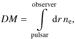 (1)where ne is the
three-dimensional free electron density. DM can be estimated by measuring the arrival time of a pulse at
different frequencies, since the time delay is proportional to DM/ν2. While there is a
vast number of known dispersion measures, very few of them are complemented by an
independent distance estimate. The NE2001 model by Cordes
& Lazio (2002) is currently the most popular model for the free electron
density of the Milky Way. It uses 1143 DM measurements, 112 of which were complemented by distance estimates of
varying quality. Additionally, it uses 269 pulsar scattering measurements, which only
provide very indirect distance constraints.
(1)where ne is the
three-dimensional free electron density. DM can be estimated by measuring the arrival time of a pulse at
different frequencies, since the time delay is proportional to DM/ν2. While there is a
vast number of known dispersion measures, very few of them are complemented by an
independent distance estimate. The NE2001 model by Cordes
& Lazio (2002) is currently the most popular model for the free electron
density of the Milky Way. It uses 1143 DM measurements, 112 of which were complemented by distance estimates of
varying quality. Additionally, it uses 269 pulsar scattering measurements, which only
provide very indirect distance constraints.
We here perform nonparametric tomography of a simulation of the Galactic free electron density from pulsar dispersion measures complemented by independent distance estimates. By nonparametric tomography we mean a reconstruction with a virtually infinite1 number of degrees of freedom using a close to minimal set of prior assumptions that only resolves structures that are supported by the data. Our assumptions are that the electron density is positive and spatially correlated and that the large-scale electron distribution only shows a variation with distance from the Galactic center and height above the Galactic plane. Both the correlation structure and the scaling behavior have to be inferred from the data. As a consequence, our reconstruction is focused on the large (kpc) scales of the Galactic free electron density. Small-scale structures such as HII regions and supernova remnants as well as spiral arms are only recovered if they are sufficiently deeply probed and constrained by the data.
Our tomography algorithm is derived from first principles in a Bayesian setting. This has the advantage that all assumptions are clearly stated as priors. Additionally, it allows us to provide uncertainty maps of our reconstructions, which are important for any subsequent scientific analysis.
To obtain a meaningful map with minimal assumptions, a data set of high quality is needed, of course. Currently, there are around 100 pulsars known with reliable (independent) distance estimates. This only allows for a nonparametric reconstruction of the largest features in the Milky Way. New measurements with the Very Long Baseline Array will soon double the number of pulsars with accurate distances (see Deller et al. 2011). However, with the planned Square Kilometer Array radio interferometer (SKA) the number of pulsars with parallax distance estimates might increase to around 10 000 (see Smits et al. 2011). In this paper we therefore investigate the feasibility of nonparametric tomography of the free electron density and demonstrate the performance of our algorithm by applying it to mock data sets similar to what the SKA might deliver. To this end, we create four Galaxy models from the NE2001 code by Cordes & Lazio (2002) with varying degrees of fluctuations and contrast as well as observational mock data sets for up to 10 000 pulsars with distance estimates of varying quality and apply our algorithm to these data sets.
The remainder of this paper is structured as follows: first, we derive our tomography algorithm in Sect. 2, explaining our notation, our underlying assumptions, and all probability density functions (PDFs) involved. Second, we explain our Galaxy models and mock observations in detail in Sect. 3. In Sect. 4 we compare the electron density distributions reconstructed from mock observations with those from the Galaxy models used to produce them. We summarize our discussion in Sect. 5.
2. Reconstruction algorithm
The reconstruction algorithm applied in this work was derived within the framework of information field theory introduced by Enßlin et al. (2009). We also follow for most parts the notation used by them. To reconstruct the Galactic free electron density from pulsar dispersion measurements, we used a filter formalism very similar to the one presented by Junklewitz et al. (2016), which in turn is based on the critical filter formalism developed by Enßlin & Weig (2010), Enßlin & Frommert (2011), and refined by Oppermann et al. (2013).
2.1. Signal model
In the inference formalism we aim to reconstruct the free electron density field
ρ, a
three-dimensional scalar field. We assume it is related to the observed dispersion measure
data DM by a linear
measurement equation subject to additive and signal-independent measurement noise,
 (2)where n is the measurement noise
and Rρ is the
application of the linear response operator R on the field ρ,
(2)where n is the measurement noise
and Rρ is the
application of the linear response operator R on the field ρ,
 (3)The response operator R describes line-of-sight
integrals through the density. It can be defined as
(3)The response operator R describes line-of-sight
integrals through the density. It can be defined as
 (4)where di is the
position of pulsar i in a coordinate system centered on the Sun, and
δ(·) is the
three-dimensional Dirac delta-distribution and
(4)where di is the
position of pulsar i in a coordinate system centered on the Sun, and
δ(·) is the
three-dimensional Dirac delta-distribution and  .
.
Formally, the free electron density is a continuous field. In practice, we reconstructed a discretized version of this field, for instance, a three-dimensional map with some pixel size. The discretized density field can be thought of as a vector of dimension Npix with each component containing the field value in a specific pixel. The dispersion data DM and the noise n can be regarded as vectors of dimension Ndata, where each component of DM contains a specific measurement result and the corresponding component of n the noise contribution to it. Thus, the response operator becomes a matrix with Npix columns and Ndata rows.
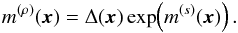
We parametrized the density as  (5)where Δ is the Galactic profile field that
describes the disk shape of the Milky Way. All deviations from the Galactic profile are
described by
(5)where Δ is the Galactic profile field that
describes the disk shape of the Milky Way. All deviations from the Galactic profile are
described by  for which we assumed no distinguished
direction or position a priori. To ensure positivity of the density, these fields were in
turn parametrized as
for which we assumed no distinguished
direction or position a priori. To ensure positivity of the density, these fields were in
turn parametrized as 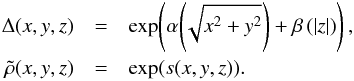 (6)Thus, Δ can only represent the vertical and radial
scaling behavior of the density and has the degrees of freedom of two one-dimensional
functions. On the other hand,
(6)Thus, Δ can only represent the vertical and radial
scaling behavior of the density and has the degrees of freedom of two one-dimensional
functions. On the other hand,  retains all degrees of freedom of a
three-dimensional field and can represent arbitrary structures. Neither Δ nor
are known a priori and will be inferred
from the data.
retains all degrees of freedom of a
three-dimensional field and can represent arbitrary structures. Neither Δ nor
are known a priori and will be inferred
from the data.
We summarize our modeling in Fig. 1. The logarithmic density ρ is parametrized by three additive components, one three-dimensional field and two one-dimensional fields. As we outline in Sects. 2.2.2 and 2.3, all three fields are assumed to follow Gaussian statistics a priori. For the 1D fields a specific correlation structure was assumed, while the correlation structure of the three-dimensional field was unknown, but assumed to be homogeneous and isotropic. Therefore, our modeling prefers smooth structures, fluctuations that scale with the density, and exponential scaling in radial and vertical directions. Of course, this is a strong simplification of the Galaxy, where the behavior of the fluctuations can depend on the phase of the interstellar medium or the position within the Galaxy, for instance. However, all of these properties can be recovered if the data demand it, since all degrees of freedom are retained. They are just not part of the prior knowledge entering our inference.
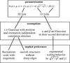 |
Fig. 1 Diagram outlining the structure of our modeling. |
2.2. Necessary probability density functions
Our goal is to derive an algorithm that yields an estimate of the logarithm of the
Galactic free electron density. Hence, we constructed the posterior PDF
 , which is the PDF for the
signal given the data set {
DM,dobs(erved)
}, using Bayes’ theorem,
, which is the PDF for the
signal given the data set {
DM,dobs(erved)
}, using Bayes’ theorem, 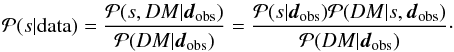 (7)On the right-hand side, we have three PDFs:
the prior
(7)On the right-hand side, we have three PDFs:
the prior  ,
the likelihood
,
the likelihood  ,
and the evidence
,
and the evidence  .
The evidence is independent of the signal and therefore automatically determined by the
normalization of the posterior. The prior and the likelihood are addressed in the
following sections. For notational convenience we drop the dependence on the observed
pulsar positions dobs throughout the rest of
this paper.
.
The evidence is independent of the signal and therefore automatically determined by the
normalization of the posterior. The prior and the likelihood are addressed in the
following sections. For notational convenience we drop the dependence on the observed
pulsar positions dobs throughout the rest of
this paper.
Throughout this section we assume the Galactic profile field to be given. We adress its inference in Sect. 2.3.
2.2.1. Likelihood
The likelihood  is the PDF
that an observation yields dispersion measures DM assuming a specific realization of the
underlying signal field s. If both the noise n and the pulsar
distances di ≡ |
di | were
known, the relation between the dispersion measure data and signal would be
deterministic,
is the PDF
that an observation yields dispersion measures DM assuming a specific realization of the
underlying signal field s. If both the noise n and the pulsar
distances di ≡ |
di | were
known, the relation between the dispersion measure data and signal would be
deterministic,  (8)with ρ(x) =
Δ(x)es(x).
We do not know the realization of the noise, nor do we aim to reconstruct it. It was
assumed to follow Gaussian statistics with zero mean and known covariance structure2,
(8)with ρ(x) =
Δ(x)es(x).
We do not know the realization of the noise, nor do we aim to reconstruct it. It was
assumed to follow Gaussian statistics with zero mean and known covariance structure2,
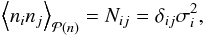 (9)where σi is the root mean
square error of the observation i, and we assumed independent measurements.
Distance information is usually given in the form of parallaxes from which distance
estimates can be derived. As all observables, these are subject to uncertainties, which
is why the information about the distances of the pulsars is described by a PDF3,
(9)where σi is the root mean
square error of the observation i, and we assumed independent measurements.
Distance information is usually given in the form of parallaxes from which distance
estimates can be derived. As all observables, these are subject to uncertainties, which
is why the information about the distances of the pulsars is described by a PDF3,  , which can be
non-Gaussian. Since we are doing inference on s, we need the noise and distance4 marginalized likelihood
, which can be
non-Gaussian. Since we are doing inference on s, we need the noise and distance4 marginalized likelihood  (10)where we assumed n and d to be independent of
s and
each other. The symbols
(10)where we assumed n and d to be independent of
s and
each other. The symbols  and
and  denote integration over the full configuration space of n and d, that is, the space of
all possible configurations (
denote integration over the full configuration space of n and d, that is, the space of
all possible configurations ( ).
).
Integration over n in Eq. (10)is trivial and yields
 (11)where
 indicates a Gaussian PDF,
  . Integration over d, however, cannot be
done analytically, but the marginalized likelihood can be approximated by a Gaussian
characterized by its first two moments in DM. The first moment is
. Integration over d, however, cannot be
done analytically, but the marginalized likelihood can be approximated by a Gaussian
characterized by its first two moments in DM. The first moment is
 (12)with
![\begin{eqnarray} \tilde{R}_i(\vec{x}) = \left\langle R_i(\vec{x}) \right\rangle_{\mathcal{P}(d)} = \int\limits_{0}^{\infty}\!\!\mathrm{d}r\ \delta\!\left( \vec{x} - r\boldsymbol{\hat{d}}_i \right)\, P[d_i>r], \end{eqnarray}](/articles/aa/full_html/2016/06/aa26717-15/aa26717-15-eq50.png) (13)where P [
di>r
] is the probability that the pulsar distance di is larger than
r. The
second moment is
(13)where P [
di>r
] is the probability that the pulsar distance di is larger than
r. The
second moment is  (14)For non-diagonal elements the second term
on the right-hand side decouples,
(14)For non-diagonal elements the second term
on the right-hand side decouples,
![\begin{eqnarray} \left\langle \left(R\rho\right)_i\left(R\rho\right)_j \right\rangle_{\mathcal{P}(d)} & =& \left\langle \left(R\rho\right)_{i\!\!\phantom{j}} \right\rangle_{\mathcal{P}(d)} \left\langle\left(R\rho\right)_j \right\rangle_{\mathcal{P}(d)}\nonumber\\[3mm] & = &\left( \tilde{R}\rho \right)_i\left( \tilde{R}\rho \right)_j \quad \mathrm{for}\quad i\neq j. \end{eqnarray}](/articles/aa/full_html/2016/06/aa26717-15/aa26717-15-eq55.png) (15)Diagonal elements yield
(15)Diagonal elements yield
![\begin{eqnarray} \left\langle \left(R\rho\right)_i\left(R\rho\right)_i \right\rangle_{\mathcal{P}(d)} & = & \int\limits_{\mathbb{R}^3}\!\!\mathrm{d}^3x\int\limits_{\mathbb{R}^3}\!\!\mathrm{d}^3y \ \rho(\vec{x})\rho(\vec{y}) \nonumber\\[3mm] && \times\left\langle R_i(\vec{x}) R_i(\vec{y}) \right\rangle_{\mathcal{P}(d)}, \end{eqnarray}](/articles/aa/full_html/2016/06/aa26717-15/aa26717-15-eq56.png) (16)with
(16)with
![\begin{eqnarray} \left\langle R_i(\vec{x}) R_i(\vec{y}) \right\rangle_{\mathcal{P}(d)} & = & \int\limits_{0}^{\infty}\mathrm{d}r\int\limits_{0}^{\infty}\mathrm{d}r'\ \delta(\vec{x}-r\boldsymbol{\hat{d}}_i) \delta(\vec{y}-r'\boldsymbol{\hat{d}}_i) \nonumber\\ && \times P[d_i>\max(r,r')]. \end{eqnarray}](/articles/aa/full_html/2016/06/aa26717-15/aa26717-15-eq57.png) (17)Using these first two moments, we can
approximate5 the likelihood
by a Gaussian
(17)Using these first two moments, we can
approximate5 the likelihood
by a Gaussian
 with
with  (18)where6
![\begin{eqnarray} F^{(i)}(\vec{x},\vec{y}) & := &\left\langle R_i(\vec{x})R_i(\vec{y})\right\rangle _{\mathcal{P}(d_i)} - \tilde{R}_i(\vec{x})\tilde{R}_i(\vec{y}) \nonumber\\[3mm] & = & \int\limits_{0}^{\infty}\mathrm{d}r\int\limits_{0}^{\infty}\mathrm{d}r'\ \delta(\vec{x}-r\boldsymbol{\hat{d}}_i) \delta(\vec{y}-r'\boldsymbol{\hat{d}}_i) \nonumber\\[3mm] &&\quad \times P[d_i>\max(r,r')]P[d_i<\min(r,r')]. \end{eqnarray}](/articles/aa/full_html/2016/06/aa26717-15/aa26717-15-eq60.png) (19)The noise covariance matrix of this
effective likelihood is signal dependent, which increases the complexity of the
reconstruction problem. Therefore, we approximated the density in Eq. (18)by its posterior mean,
(19)The noise covariance matrix of this
effective likelihood is signal dependent, which increases the complexity of the
reconstruction problem. Therefore, we approximated the density in Eq. (18)by its posterior mean,  (20)Since
 depends on
  this yields a set of equations that need
to be solved self-consistently (see Sect. 2.4).
this yields a set of equations that need
to be solved self-consistently (see Sect. 2.4).
2.2.2. Priors
The signal field s is unknown a priori, but we assumed that it has
some correlation structure. We describe this correlation structure by moments up to
second order in s. The principle of maximum entropy therefore
requires that our prior probability distribution has a Gaussian form,
 (21)with some unknown correlation structure,
 (22)The first moment of s is set to zero because
it can be absorbed into Δ(x). This means that the a priori
mean of s
is contained in Δ(x).
(22)The first moment of s is set to zero because
it can be absorbed into Δ(x). This means that the a priori
mean of s
is contained in Δ(x).
A priori, our algorithm has no preferred direction or position for s. This reduces the
number of degrees of freedom of the correlation structure S. It is fully described
by a power spectrum p(k),
 (23)where S(k) is the projection
operator onto the spectral band k, with its Fourier transform defined as
(23)where S(k) is the projection
operator onto the spectral band k, with its Fourier transform defined as
 (24)with
![\begin{eqnarray} \mathbb{1}_k\!\left(|\vec{q}|\right) = \begin{cases} 1 & \mathrm{for}\ \ |\vec{q}|=k \\[3mm] 0 & \mathrm{otherwise}. \end{cases} \end{eqnarray}](/articles/aa/full_html/2016/06/aa26717-15/aa26717-15-eq73.png) (25)The power spectrum p(k),
however, is still unknown. The prior for the power spectrum is constructed out of two
parts: First, an inverse gamma distribution ℐ(p(k);αk,qk)
for each k-bin (see Appendix A), which is a conjugate prior for a Gaussian PDF, second a Gaussian
cost-function that punishes deviations from power-law spectra (see Oppermann et al. 2013),
(25)The power spectrum p(k),
however, is still unknown. The prior for the power spectrum is constructed out of two
parts: First, an inverse gamma distribution ℐ(p(k);αk,qk)
for each k-bin (see Appendix A), which is a conjugate prior for a Gaussian PDF, second a Gaussian
cost-function that punishes deviations from power-law spectra (see Oppermann et al. 2013),
 (26)T is an operator that fulfills
  (27)and σp is a parameter that
dictates how smooth the power spectrum is expected to be. In our paper log refers to the natural logarithm. We
explain our choice of the parameters αk, qk, and σp in Appendix A.
(27)and σp is a parameter that
dictates how smooth the power spectrum is expected to be. In our paper log refers to the natural logarithm. We
explain our choice of the parameters αk, qk, and σp in Appendix A.
2.2.3. Power spectrum posterior
With the signal and power spectrum priors, we can derive a posterior for the power
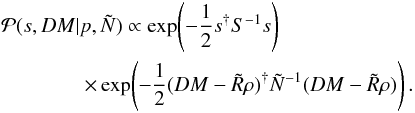
spectrum,  (28)We calculated the integral using a saddle
point approximation up to second order around the maximum for the s-dependent part,
(28)We calculated the integral using a saddle
point approximation up to second order around the maximum for the s-dependent part,
![\begin{eqnarray} \mathcal{P}(DM|s)\,\mathcal{G}(s,S) && \approx \mathcal{P}(DM|m)\,\mathcal{G}(m,S)\,\mathrm{e}^{-\frac{1}{2}(s-m)^{\dagger} D^{-1}(s-m)}\nonumber\\[3mm] && \propto \mathcal{G}(m,S)\,\mathrm{e}^{-\frac{1}{2}(s-m)^{\dagger} D^{-1}(s-m)}, \end{eqnarray}](/articles/aa/full_html/2016/06/aa26717-15/aa26717-15-eq84.png) (29)where m and D are defined as
m(s) and
D(s) in Sect. 2.2.4 and only s − and p-dependent factors are
kept after the proportionality sign. With this approximation we arrive at
(29)where m and D are defined as
m(s) and
D(s) in Sect. 2.2.4 and only s − and p-dependent factors are
kept after the proportionality sign. With this approximation we arrive at
 (30)Maximizing this PDF with respect to
log (p)
(see Oppermann et al. 2013) leads to
(30)Maximizing this PDF with respect to
log (p)
(see Oppermann et al. 2013) leads to
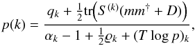 (31)where
 is the number of degrees of freedom in
the spectral band k. This formula for the power spectrum
p(k) should be solved
self-consistently because m and D depend on p(k) as
well. Thus we arrive at an iterative scheme, where we look for a fixed point of Eq.
(31).
is the number of degrees of freedom in
the spectral band k. This formula for the power spectrum
p(k) should be solved
self-consistently because m and D depend on p(k) as
well. Thus we arrive at an iterative scheme, where we look for a fixed point of Eq.
(31).
2.2.4. Signal posterior
The signal posterior can be expressed as
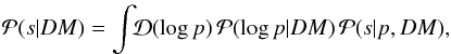 (32)where
 is the
signal posterior with a given power spectrum. Instead of calculating the marginalization
over log p,
we used Eq. (31)for the power spectrum;
that is, we approximated
is the
signal posterior with a given power spectrum. Instead of calculating the marginalization
over log p,
we used Eq. (31)for the power spectrum;
that is, we approximated  by a Dirac
peak at its maximum. This procedure is known as the empirical Bayes method. The signal
posterior with a given power spectrum is proportional to the product of the signal prior
and the likelihood (see Eq. (7)),
by a Dirac
peak at its maximum. This procedure is known as the empirical Bayes method. The signal
posterior with a given power spectrum is proportional to the product of the signal prior
and the likelihood (see Eq. (7)),
 (33)However, as has been demonstrated in Sects.
2.2.3 and 2.2.1, S and
(33)However, as has been demonstrated in Sects.
2.2.3 and 2.2.1, S and  depend on the mean and the covariance of
 leading to a circular dependence that
needs to be solved self-consistently.
leading to a circular dependence that
needs to be solved self-consistently.
We approximate the mean of the posterior by minimizing the joint Hamiltonian
 with respect to s,
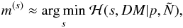 (34)and its covariance by the inverse Hessian
at that minimum,
(34)and its covariance by the inverse Hessian
at that minimum,  (35)These estimates are the maximum a
posteriori (MAP) estimates of s. Consequently, m(ρ) and
D(ρ) are estimated as
(35)These estimates are the maximum a
posteriori (MAP) estimates of s. Consequently, m(ρ) and
D(ρ) are estimated as
 (36)and
 (37)S is then constructed as
 (38)with p(k)
given by Eq. (31).
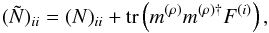
is constructed using Eqs. (18)and (20)as
(38)with p(k)
given by Eq. (31).
is constructed using Eqs. (18)and (20)as  (39)where δij is the Kronecker
delta.
(39)where δij is the Kronecker
delta.
2.3. Galactic profile inference
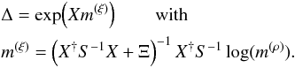
To infer the Galactic profile field Δ, we introduce  . The Galactic profile is to capture the
most prominent symmetries of a disk galaxy, namely its rotational symmetry and the scaling
behavior with radial distance from the Galactic center and vertical distance from the
Galactic plane. Using Eq. (6),
μ ≡ log (Δ)
becomes
. The Galactic profile is to capture the
most prominent symmetries of a disk galaxy, namely its rotational symmetry and the scaling
behavior with radial distance from the Galactic center and vertical distance from the
Galactic plane. Using Eq. (6),
μ ≡ log (Δ)
becomes  (40)where α and β are one-dimensional
functions describing the average behavior with respect to the radial distance and the
vertical distance from the Galactic center. Including the shift by μ from s to
(40)where α and β are one-dimensional
functions describing the average behavior with respect to the radial distance and the
vertical distance from the Galactic center. Including the shift by μ from s to
 yields the signal prior
 (41)We do not wish to assume specific functions
α and
β, but to
infer them. To this end we chose a Gaussian prior,
(41)We do not wish to assume specific functions
α and
β, but to
infer them. To this end we chose a Gaussian prior,
 (42)with the second derivative of α (or β, respectively) as the
argument. This prior prefers linear functions for α and β and thus Galactic profile
fields with an exponential fall-off (or rise). To simplify the notation, we defined
ξ(r, |
z | ) = (α(r),β( |
z | ))T and introduced
the linear operators Ξ and
X, where
(42)with the second derivative of α (or β, respectively) as the
argument. This prior prefers linear functions for α and β and thus Galactic profile
fields with an exponential fall-off (or rise). To simplify the notation, we defined
ξ(r, |
z | ) = (α(r),β( |
z | ))T and introduced
the linear operators Ξ and
X, where
 (43)and
 (44)Now we can write the Hamiltonian of
ξ given a
specific electron density as
(44)Now we can write the Hamiltonian of
ξ given a
specific electron density as  (45)with
  and
and
 . Since this Hamiltonian is a quadratic
form in ξ,
the mean of the corresponding Gaussian PDF is
. Since this Hamiltonian is a quadratic
form in ξ,
the mean of the corresponding Gaussian PDF is
 (46)
(46)
2.4. Filter equations
Using the posterior estimates presented in the previous section, we arrive at the following iterative scheme for reconstructing the density ρ:
-
1.
Make an initial guess for the power spectrum (e.g., some power law) and the additive term in the noise covariance (e.g., simple relative error propagation).
-
2.
With the current estimates for p and
the Hamiltonian,
 , is
, is
 (47)where theasterisk denotes point-wise
multiplication in position space.
(47)where theasterisk denotes point-wise
multiplication in position space. -
3.
The MAP estimate of this Hamiltonian is calculated as
 (48)with the covariance estimate (see
Appendix B)
(48)with the covariance estimate (see
Appendix B)  (49)
(49) -
4.
The updated power spectrum is the solution (with respect to p(k)) of the equation
 (50)
(50) -
5.
The updated effective noise covariance is calculated as
 (51)with
 (52)
(52) - 6.
-
7.
Repeat from step 2 until convergence is reached.
When the solution of this set of equations is converged, the estimate of the density
ρ is
 (54)where the confidence interval σ(ρ) is defined as
 (55)
(55)
3. Application to simulated data
To test the reconstruction of the Galactic free electron density distribution with the SKA, we generated mock data sets of pulsars with various distance uncertainties. We simulated pulsar populations using the PSRPOPpy package by Bates et al. (2014), which is based on the pulsar population model by Lorimer et al. (2006). The generated populations take the observational thresholds of the SKA into account (mid-frequency). These data sets sample modified versions of the NE2001 model by Cordes & Lazio (2002) through dispersion measures.
3.1. Galaxy model
We deactivated7 all local ISM components as well as all clumps and voids in the NE2001 model. We kept the clump in the Galactic center, since it is the only one at a distinguished position. We evaluated8 the resulting free electron density model in a 512 × 512 × 64 pixel grid centered on the Galactic center with a pixel edge length of 75 pc. This means that our model extends out to 2400 pc from the Galactic plane. We assumed a density of zero outside of this regime when calculating the dispersion measures. The resulting density field is very smooth. We generated three Gaussian random fields that follow a power-law distribution with a spectral index9 of −4.66, but have different fluctuation amplitudes. We verified that the Sun is located in an underdensity in these random fields. Then we added these three random field maps to our smooth map of log (ne) to create three different modified versions of NE2001. In Fig. 2 we depict the power spectra of the smooth NE2001 field (without local features, clumps, and voids) and the power spectra of its three modified versions.
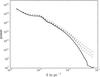 |
Fig. 2 Power spectrum of the NE2001 field without local features, clumps, and voids compared to the three unenhanced Galaxy models. The thick solid line depicts the NE2001 spectrum, the thin dashed lines depict the spectra of the models with strong, medium, and weak fluctuations (from top to bottom). To calculate the spectra, the density peak in the Galactic center is masked. |
3.1.1. Contrast-enhanced model
The three Galaxy models we generated from NE2001 have relatively little contrast in the sense that under- and overdense regions differ by relatively moderate factors. For example, the density in the region between the Perseus and Carina-Sagittarius arm where the Sun is located is only a factor of three lower than in the Perseus arm itself. Since the Perseus arm is a less than 1 kpc in width, any excess dispersion measure that is due to the arm can also be explained by an underestimated pulsar distance for many lines of sight. In consequence, we expect the reconstruction quality to improve if the input model has higher contrast. Therefore, we prepared one additional model with enhanced contrast. To this end, we took the input model with medium-strength fluctuations as described above. We divided out the scaling behavior in radial and vertical directions using the scale heights from NE2001. We squared the density and divided it by a constant to ensure that the mean density in the Galactic plane remains unchanged10. Finally we multiplied the resulting density with the scaling functions to restore the original scaling in radial and vertical directions.
This procedure yielded a Galaxy model sharing the same morphology and scaling behavior as the input model. Averaged over the lines of sight, the value of the dispersion measures is roughly unchanged. But the contrast is twice as strong, that is, the previously mentioned factor between the density in the Perseus arm and the inter-arm region is now squared from 3 to 9. We show a picture of the density in the Galactic plane of this model in Sect. 4.1, where we compare it with its reconstruction.
3.2. Simulated population and survey
We used the SKA template in the PSRPOPpy package, but reduced the maximum declination in equatorial coordinates to 50° (this is due to the SKAs position on the Southern Hemisphere, see e.g. Smits et al. 2009). This yielded a detected population of roughly 14 000 pulsars. Out of these, we took the first 1000, 5000, or 10 000 pulsars as our test populations. The population was not ordered in any sense, which means that the first 1000 pulsars, for example, represent a random sample from the whole detected population. In reality, the Malmquist bias preferentially selects pulsars that lie close to the Sun. We chose a random selection, however, to see the effect of the population size on the quality of the reconstruction more clearly. In Fig. 3 we depict the population of 10 000 pulsars projected onto the sky. The pulsars are concentrated toward the center of the Galaxy. The gap in the equatorial Northern Hemisphere is clearly evident in the left part of the plot.
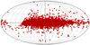 |
Fig. 3 Positions of the simulated 10 000 pulsars on the sky in Galactic coordinates. |
3.3. Simulated dispersion measures and distances
We calculated the line integrals through the Galaxy models from the positions generated by the PSRPOPpy package to the Sun to generate simulated dispersion measures. We added Gaussian random variables to the pulsar distances to simulate measurement uncertainties of the distances. For each pulsar we generated one random number and scale this to 5%, 15%, or 25% of the distance of the pulsar. In reality the distance PDF would be non-Gaussian. The exact form depends on the combination of observables that are used to infer the distance. We used Gaussian PDFs for simplicity. As long as the real distance PDFs are unimodal, we do not expect this choice to have a significant effect on our study. We did not simulate additional measurement noise for the dispersion measures because it is expected to be small compared to the distance uncertainty. This leaves us with a number of data sets that are described in Table 1. In this table we omit the combinations of 1000 pulsars at 25% distance error (because we do not hope for a good reconstruction in that case) and 10 000 pulsars at 5% distance error (because we deem it to be too unrealistic).
Types of data sets simulated for all Galaxy models.
The aforementioned measurement scenarios were chosen to see the effect of the population size and the distance error on the reconstruction in isolation. A more realistic setting is of course a mix of distance uncertainties where more distant pulsars have larger distance errors on average. We therefore created one additional measurement scenario for 10 000 pulsars, where we assigned the uncertainty magnitude of each pulsar randomly11. The distance uncertainties are distributed as shown in Fig. 4. In this measurement set, 2969 pulsars have a 5% distance error, 3400 pulsars have a 15% distance error, and 3631 pulsars have a 25% distance error. Throughout the rest of this paper we refer to this data set as the mixed data set.
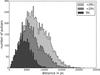 |
Fig. 4 Histogram showing the distance uncertainty distribution with respect to the distance from the Sun in the mixed measurement set. |
A very rough estimate of the scales that we can hope to resolve is given by the mean distance between neighboring pulsars and the average misplacement that is due to distance errors. The mean distance between neighboring pulsars is 490 pc for 1000, 290 pc for 5000, and 230 pc for 10 000 pulsars. The average misplacement is 380 pc for 5%, 1100 pc for 15%, and 1900 pc for 25% distance errors and 1300 pc for the mixed data set. Interpreting these distances as independent uncertainties, we can combine them by adding the squares and taking the square root. This provides a rough estimate of sampling distances. In Table 2 we list these distances for each data set.
Estimated sampling distances for each data set.
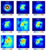 |
Fig. 5 Several reconstructions of the Galaxy model with medium strength fluctuations. All panels show top-down views of the electron density in the Galactic plane using a linear color scale in units of cm-3. The panels span 36 000 pc in each dimension. The Sun is located at the white dot depicted in each panel. The rows show reconstructions with distance errors of 25%, 15%, and 5% (from top to bottom). The columns show reconstructions with 1000, 5000, and 10 000 pulsars (from left to right). The layout follows Table 1. The top left panel shows the original input model (modified NE2001). The bottom right panel shows the reconstruction of the mixed measurement set. |
3.4. Algorithm setup
The algorithm was set up in a 128 × 128 ×
48 pixel grid centered on the Galactic center with pixel
dimensions12 of 281.25 pc × 281.25 pc × 250 pc. While the
dispersion measures in our data sets were free from instrumental noise, the noise was
assumed to be 2% in the
algorithm. This provides a lower limit for the effective noise covariance (Eq. (18)) and thus ensures stability of the
inference without losing a significant amount of precision. The initial guess for the
power spectrum is a broken power law with an exponent of −3.6613. For the propagated distance uncertainty it is
![\begin{eqnarray} \sigma_i = \frac{\sqrt{\mathrm{Var}[d_i]}}{d_i} DM_i, \end{eqnarray}](/articles/aa/full_html/2016/06/aa26717-15/aa26717-15-eq175.png) (56)where di is the distance of the
pulsar (see Sect. 2.2.1). The initial guesses of the
Galactic profile functions14 are
(56)where di is the distance of the
pulsar (see Sect. 2.2.1). The initial guesses of the
Galactic profile functions14 are
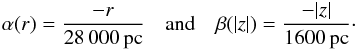 (57)We discuss the convergence and final values
of the power spectrum, effective errors, and profile functions in Appendix C.
(57)We discuss the convergence and final values
of the power spectrum, effective errors, and profile functions in Appendix C.
4. Simulation evaluation
Our algorithm accounts for most of the variance in the data while regularizing the result to avoid overfitting. Most of the reconstructions shown in this section have corresponding reduced χ2 values close to 1, indicating that they show all structures that are sufficiently well constained by the data. We discuss the reduced χ2 values in detail in Appendix D.
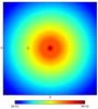 |
Fig. 6 Recovered Galactic profile in the Galactic plane. Shown is a top-down view the Galaxy as in Fig. 5, but here in logarithmic color scale. The input model had medium strength fluctuations, it was recovered using 5000 pulsars with 5% distance uncertainty (corresponding to the bottom middle panel in Fig. 5). Other fluctuation strengths and data sets would yield a very similar image. |
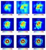 |
Fig. 7 Reconstructions of the three Galaxy models with fluctuation strengths using 5000 pulsars. All panels show top-down views of the electron density in the Galactic plane using a linear color scale in units of cm-3. The panels span 36 000 pc in each dimension. The rows show reconstructions with distance errors of 15% and 5% (from top to bottom). Bottom row: original Galaxy models. Columns: reconstructions and original input models (modified NE2001) with weak, medium, and strong fluctuations (from left to right). |
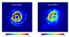 |
Fig. 8 Input model (left) and reconstruction (right) of the contrast-enhanced Galaxy model using 5000 pulsars with distance uncertainties of 5%. Both panels show top-down views of the electron density in the Galactic plane using a linear color scale in units of cm-3. The panels span 36 000 pc in each dimension. |
4.1. Density in the midplane
The simulations show that with the amount of pulsars with reliable distance estimates that the SKA should deliver reconstruction of the free electron density in the vicinity of the Sun becomes feasible (see Fig. 5). However, small-scale features are difficult to identify in the reconstruction. Identifying spiral arms remains challenging as well, especially beyond the Galactic center. To resolve the spiral arms in the vicinity of the Sun, between 5000 and 10 000 pulsars with distance accuracies between 5% and 15% are needed. As is evident from the figure, small distance uncertainties increase the quality of the reconstruction significantly. The reconstruction from 5000 pulsars with 5% distance uncertainty is better in quality than the one from 10 000 pulsars with 15% distance uncertainty15. All reconstructions smooth out small-scale structure in the electron density, for example, at the Galactic center. If an overdensity appears at the wrong location, this indicates that the data do not constrain the overdensity well. For completeness we also show the recovered Galactic profile in the Galactic plane for 5000 pulsars with 5% distance uncertainty in Fig. 6. For other data sets the plot would look very similar. In Appendix E we show a reconstruction where the Galactic profile and the correlation structure a known a priori and in Appendix F we show and discuss the uncertainty estimate of the algorithm.
In Fig. 7 we compare the performance of the reconstruction algorithm for the three input model fluctuation strengths using 5000 pulsars with 5% and 15% distance uncertainty. The strength of the fluctuations clearly does not influence the quality of the reconstructions by much. The reconstructions of the models with stronger fluctuations exhibit stronger fluctuations as well, while all reconstruction omit or smear features to a similar degree. However, it clearly becomes more difficult to reconstruct the Perseus arm toward the Galactic anticenter if the fluctuations in the electron density are strong. This is to be expected because the spiral arm is also harder to recognize in the original model as the fluctuations become stronger.
In Fig. 8 we show the contrast-enhanced Galaxy model and its reconstruction using 5000 pulsars with distance uncertainties of 5%. As is clear from the figure, the algorithm is able to resolve much more detailed structure than the reconstruction of the unenhanced Galaxy model (bottom middle panel in Fig. 5). We stress that the pulsar population and their distance uncertainties are exactly the same for both cases. The increase in quality comes merely from the increased contrast and the resulting stronger imprint of under- and overdensities in the dispersion data. Therefore, we conclude that if the contrast of the real Galaxy is much stronger than in NE2001, our algorithm could resolve the Galaxy much better that the study on NE2001 indicates.
4.2. Vertical fall-off
A quantity of interest in any model of the Galactic free electron density is the drop-off of the average density with respect to distance from the Galactic plane. This behavior is shown in Fig. 9, which displays a vertical cut through the Galactic profile reconstructed using 5000 pulsars with 5% distance uncertainty.
In our parametrization the function β in Eq. (40)describes the average log-density at a certain distance from the Galactic plane. In Fig. 10 we show the estimates for β corresponding to the reconstructions shown in Fig. 5 along with their uncertainties (see Appendix G for their calculation). The uncertainty regions reflect that a vertical fall-off can be explained by a global profile as well as by density fluctuations close to the Sun. This uncertainty is nearly independent of the quality of the data set, but depends on the strength of fluctuations on kpc scales. These are always present unless the data probe a simplistic disk. Therefore, there is a lower bound of precision to which our algorithm can determine the vertical fall-off behavior. We compared the reconstructed vertical scaling to a global and a local estimate generated from the original input model. The global estimate describes vertical fall-off throughout the whole model, whereas the local estimate describes the vertical fall-off close to the Sun16. For completeness we also provide best-fitting scale heights for exponential fall-offs in the figure, that is, we fit the vertical scaling to ne ∝ e− | z | /Hz. The uncertainties of these estimates were calculated by performing the fit on multiple posterior samples of β. The local and global estimate both have significantly lower scale heights than the 950 pc from NE2001 (thick disk). This is probably due to the combination of the thick disk with the thin disk of NE2001 (which has a scale height of 140 pc). As is evident from the figure, the reconstructed z-profile is dominated by the local behavior of the density and agrees with it within the error bars throughout all data sets17 for the regime | z | < 2400 pc. However, the width of the uncertainty region prohibits a clear decision whether the vertical fall-off follows a single exponential function or a thick disk and a thin disk, as is the case for NE2001. In our input model we set ne to zero for | z | > 2400 pc. In this regime our reconstruction is unreliable.
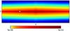 |
Fig. 9 Vertical cut through the same Galactic profile as in Fig. 6. Shown is the slice containing the Sun (white dot) and the Galactic center (middle). The image spans 36 kpc × 12 kpc. The color scale is logarithmic. |
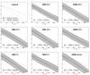 |
Fig. 10 Recovered z-dependent fall-off in logarithmic units (function β in Eq. (40)), input model with medium strength fluctuations. Top left panel: global z-profile (dashed line) as well as the local z-profile (dotted line). In all other panels the solid line is the recovered z-profile while the global and local z-profile are replotted (in dashed and dotted respectively). The gray areas indicate the 1σ uncertainty around the recovered z-profile. In the bottom left corner of each panel: best fitting exponential scale height (and its 1σ uncertainty for the reconstructions). |
5. Summary and conclusions
We presented an algorithm that performs nonparametric tomography of the Galactic free electron density using pulsar dispersion measures and distances. The algorithm produces a three-dimensional map and a corresponding uncertainty map. It automatically estimates the correlation structure and the scales of the disk shape, requiring only approximate initial guesses for them. The uncertainties of pulsar distance estimates are consistently propagated.
Using our algorithm, we investigated the feasibility of nonparametric tomography with the upcoming Square Kilometer Array. To this end, we created three Galaxy models with various fluctuation strengths and one with enhanced contrast and simulated mock observations of these models using between 1000 and 10 000 pulsars. Our results indicate that with the amount of pulsars that the SKA is expected to deliver, nonparametric tomography becomes feasible. However, detecting spiral arms in the free electron density from pulsar dispersion measures alone remains challenging if the input model has unenhanced contrast. We find that to distinguish the spiral arms in the vicinity of the Sun, between 5000 and 10 000 pulsars with distance accuracies of between 5% and 15% are needed. The vertical fall-off behavior of the free electron density was recovered for all mock data sets we investigated. However, a clear decision whether the vertical fall-off of free electron density is best described by a single exponential function or a thick disk and a thin disk could not be made by our algorithm.
One way to increase the sensitivity of the algorithm for Galactic features would be to include them into the prior description. By including higher order statistics (non-Gaussian priors), the inference could be made more sensitive for spiral arm structures in the electron density. In cosmology, for example, higher order statistics allowed for a better recovery of cosmological filaments (e.g., Jasche & Wandelt 2013). Modeling HII regions and supernova remnants is also beyond the scope of Gaussian statistics. Another approach would be to include parametrized structures that are known from stellar observations, such as spatial templates for spiral arm locations. This would connect data-driven tomography (with infinite degrees of freedom) with classical model fitting.
The algorithm can also be used for other tomography problems with line-of-sight measurements, such as stellar absorption coefficients. It could also be extended to infer vector fields, enabling inference of the Galactic magnetic fields from pulsar rotation measures. Furthermore, a joint reconstruction of the Galactic free electron density and the magnetic field using pulsar dispersion, measures, pulsar rotation measures, and extragalactic Faraday sources needs to be investigated.
We assumed here that the distance PDF is correctly derived from the parallax PDF taking Lutz-Kelker bias into account (see Verbiest et al. 2010).
To obtain the three-dimensional free electron density from the compiled NE2001 code, we evaluated two positions in each pixel that have parallel line-of-sight vectors. The difference between their dispersion measures divided by the difference of their distance to the Sun was then taken as the free electron density in that pixel.
Each pulsar was assigned probabilities to belong to either the 5%, the 15%, or the 25% set. The probabilities depend on the pulsar distance, making more distant pulsars more likely to have higher uncertainties. The pulsar was then randomly assigned to an uncertainty set according to the probabilities.
We might have used any power spectrum as an initial guess. It has negligible influence on the final result (see Appendix C). The index of −3.66 corresponds to Kolmogorov turbulence in three dimensions. Such a power spectrum produces spatially correlated structures while permitting fluctuations on all scales.
The global estimate was calculated by averaging the logarithmic density at fixed vertical distances over the whole horizontal plane. The local estimate was calculated by averaging the logarithmic density at fixed vertical distances in a sub-area of the horizontal plane, which is centered on the Sun and has a size of 1500 pc × 1500 pc.
Acknowledgments
We wish to thank Niels Oppermann and Marco Selig for fruitful collaboration and advice. We also wish to thank Henrik Junklewitz, Jimi Green, Jens Jasche and Sebastian Dorn for useful discussions. The calculations were realized using the NIFTY18 package by Selig et al. (2013). Some of the minimizations described in Sect. 2.4 were performed using the L-BFGS-B algorithm (Byrd et al. 1995). We acknowledge the support by the DFG Cluster of Excellence “Origin and Structure of the Universe”. The simulations have been carried out on the computing facilities of the Computational Center for Particle and Astrophysics (C2PAP). We are grateful for the support by Frederik Beaujean through C2PAP. This research has been partly supported by the DFG Research Unit 1254 and has made use of NASA’s Astrophysics Data System.
References
- Bates, S. D., Lorimer, D. R., Rane, A., & Swiggum, J. 2014, MNRAS, 439, 2893 [NASA ADS] [CrossRef] [Google Scholar]
- Berry, M., Ivezić, Ž., Sesar, B., et al. 2012, ApJ, 757, 166 [NASA ADS] [CrossRef] [Google Scholar]
- Byrd, R. H., Lu, P., & Nocedal, J. 1995, SIAM J. Sci. Stat. Comput., 16, 1190 [Google Scholar]
- Cordes, J. M., & Lazio, T. J. W. 2002, ArXiv e-prints [arXiv:astro-ph/0207156] [Google Scholar]
- Deller, A. T., Brisken, W. F., Chatterjee, S., et al. 2011, in 20th Meeting of the European VLBI Group for Geodesy and Astronomy, held in Bonn, Germany, March 29−30, 2011, Institut für Geodäsie und Geoinformation, Rheinischen Friedrich-Wilhelms-Universität Bonn, 178, eds. W. Alef, S. Bernhart, & A. Nothnagel, 178 [Google Scholar]
- Enßlin, T. A., & Frommert, M. 2011, Phys. Rev. D, 83, 105014 [NASA ADS] [CrossRef] [Google Scholar]
- Enßlin, T. A., & Weig, C. 2010, Phys. Rev. E, 82, 051112 [NASA ADS] [CrossRef] [Google Scholar]
- Enßlin, T. A., Frommert, M., & Kitaura, F. S. 2009, Phys. Rev. D, 80, 105005 [NASA ADS] [CrossRef] [Google Scholar]
- Gaensler, B. M., Madsen, G. J., Chatterjee, S., & Mao, S. A. 2008, PASA, 25, 184 [NASA ADS] [CrossRef] [Google Scholar]
- Jansson, R., & Farrar, G. R. 2012a, ApJ, 757, 14 [NASA ADS] [CrossRef] [Google Scholar]
- Jansson, R., & Farrar, G. R. 2012b, ApJ, 761, L11 [NASA ADS] [CrossRef] [Google Scholar]
- Jasche, J., & Wandelt, B. D. 2013, MNRAS, 432, 894 [NASA ADS] [CrossRef] [Google Scholar]
- Junklewitz, H., Bell, M. R., Selig, M., & Enßlin, T. A. 2016, A&A, 586, A76 [NASA ADS] [CrossRef] [EDP Sciences] [Google Scholar]
- Kalberla, P. M. W., & Kerp, J. 2009, ARA&A, 47, 27 [NASA ADS] [CrossRef] [Google Scholar]
- Lallement, R., Vergely, J.-L., Valette, B., et al. 2014, A&A, 561, A91 [NASA ADS] [CrossRef] [EDP Sciences] [Google Scholar]
- Lorimer, D. R., Faulkner, A. J., Lyne, A. G., et al. 2006, MNRAS, 372, 777 [NASA ADS] [CrossRef] [Google Scholar]
- Oppermann, N., Selig, M., Bell, M. R., & Enßlin, T. A. 2013, Phys. Rev. E, 87, 032136 [NASA ADS] [CrossRef] [Google Scholar]
- Sale, S. E., & Magorrian, J. 2014, MNRAS, 445, 256 [NASA ADS] [CrossRef] [MathSciNet] [Google Scholar]
- Schnitzeler, D. H. F. M. 2012, MNRAS, 427, 664 [NASA ADS] [CrossRef] [Google Scholar]
- Selig, M., Bell, M. R., Junklewitz, H., et al. 2013, A&A, 554, A26 [NASA ADS] [CrossRef] [EDP Sciences] [Google Scholar]
- Smits, R., Kramer, M., Stappers, B., et al. 2009, A&A, 493, 1161 [NASA ADS] [CrossRef] [EDP Sciences] [Google Scholar]
- Smits, R., Tingay, S. J., Wex, N., Kramer, M., & Stappers, B. 2011, A&A, 528, A108 [NASA ADS] [CrossRef] [EDP Sciences] [Google Scholar]
- Sun, X.-H., & Reich, W. 2010, RA&A, 10, 1287 [Google Scholar]
- Sun, X. H., Reich, W., Waelkens, A., & Enßlin, T. A. 2008, A&A, 477, 573 [NASA ADS] [CrossRef] [EDP Sciences] [Google Scholar]
- Taylor, J. H., & Cordes, J. M. 1993, ApJ, 411, 674 [NASA ADS] [CrossRef] [Google Scholar]
- Verbiest, J. P. W., Lorimer, D. R., & McLaughlin, M. A. 2010, MNRAS, 405, 564 [NASA ADS] [Google Scholar]
Appendix A: Parameters of the power spectrum prior
The inverse gamma distribution is defined as
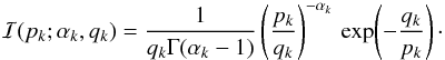 (A.1)The mean and variance of this distribution
are
(A.1)The mean and variance of this distribution
are  (A.2)There are three properties of the prior that
we wish to fulfill by choosing αk and qk. The prior of the
monopole p0, which corresponds to the variance of a
global prefactor of the density, should be close to Jeffreys prior, that is, the limit
α0 →
1, q0 → 0. The reason for this is that we
need the algorithm to stay consistent if the units are changed, for instance, from
pc to kpc. These changes introduce a global
prefactor in front of the density. Jeffreys prior has no preferred scale because it is
flat for log p0 and therefore all prefactors are
equally likely a priori. For other k-bins the parameters should favor, but not
enforce, falling power spectra. Furthermore, since p(k) is
the average power of many independent Fourier components, its a priori variance should be
inversely proportional to ϱk (the amount of
degrees of freedom in the respective k-bin), while thea priorimean should be independent
of ϱk. We therefore set
the parameters as
(A.2)There are three properties of the prior that
we wish to fulfill by choosing αk and qk. The prior of the
monopole p0, which corresponds to the variance of a
global prefactor of the density, should be close to Jeffreys prior, that is, the limit
α0 →
1, q0 → 0. The reason for this is that we
need the algorithm to stay consistent if the units are changed, for instance, from
pc to kpc. These changes introduce a global
prefactor in front of the density. Jeffreys prior has no preferred scale because it is
flat for log p0 and therefore all prefactors are
equally likely a priori. For other k-bins the parameters should favor, but not
enforce, falling power spectra. Furthermore, since p(k) is
the average power of many independent Fourier components, its a priori variance should be
inversely proportional to ϱk (the amount of
degrees of freedom in the respective k-bin), while thea priorimean should be independent
of ϱk. We therefore set
the parameters as  (A.3)where kmin is the
first non-zero k-value and f is a prefactor, which
defines a lower cut-off of the power spectrum calculated in Eq. (31). The choice of f does not influence the
result as long as it is suitably low, but higher f accelerate the
convergence of the algorithm. The denominator of 100kmin before
ϱk is chosen to
introduce a preference for falling power spectra starting two orders of magnitude from the
fundamental mode kmin (we note that 1 is subtracted in
Eq. (27)). As long as the denominator is
not too small, it has very little influence on the result of the algorithm, but smaller
denominators increase the convergence speed. We found 100kmin to be a
good compromise.
(A.3)where kmin is the
first non-zero k-value and f is a prefactor, which
defines a lower cut-off of the power spectrum calculated in Eq. (31). The choice of f does not influence the
result as long as it is suitably low, but higher f accelerate the
convergence of the algorithm. The denominator of 100kmin before
ϱk is chosen to
introduce a preference for falling power spectra starting two orders of magnitude from the
fundamental mode kmin (we note that 1 is subtracted in
Eq. (27)). As long as the denominator is
not too small, it has very little influence on the result of the algorithm, but smaller
denominators increase the convergence speed. We found 100kmin to be a
good compromise.
The parameter σp in Eq. (27)describes how much the power spectrum is expected to deviate from a power law. We chose σp = 1. If the power spectrum is locally described by a power law, σp = 1 means that the typical change of the exponent within a factor of e in k should be on the order of 1.
Appendix B: Functional derivatives of the Hamiltonian
To minimize the Hamiltonian in Sect. 2.4, the first
derivative with respect to s is needed. It is
 (B.1)where the hat converts a field to a diagonal
operator in position space, for example,
(B.1)where the hat converts a field to a diagonal
operator in position space, for example,  , and we used the shorthand notations
 (B.2)The second derivative in Eq. (49)is
 (B.3)The last term in the second derivative can be
problematic because it can break the positive definiteness19 of the second derivative, which is crucial for efficiently applying inversion
techniques such as the conjugate gradient method. However, a closer inspection of the last
two terms (omitting the hats for readability)
(B.3)The last term in the second derivative can be
problematic because it can break the positive definiteness19 of the second derivative, which is crucial for efficiently applying inversion
techniques such as the conjugate gradient method. However, a closer inspection of the last
two terms (omitting the hats for readability)
 (B.4)shows that their contribution is proportional
to the difference between the real dispersion data DM and the idealized data generated by the
map,
(B.4)shows that their contribution is proportional
to the difference between the real dispersion data DM and the idealized data generated by the
map,  . These two terms counteract each other at
the minimum, and we therefore omit them to gain numerical stability. Hence the second
derivative is approximated as
. These two terms counteract each other at
the minimum, and we therefore omit them to gain numerical stability. Hence the second
derivative is approximated as  (B.5)
(B.5)
Appendix C: Convergence
In this section, we display the convergence behavior of the power spectrum, effective errors, and profile functions. For the sake of brevity, we limit the discussion to the reconstruction of the Galaxy model with fluctuations of medium strength using the data set of 5000 pulsars with a distance error of 5%. In Appendix E we show the reconstruction of this model and data set using the real power spectrum and profile functions as a benchmark on how well our iterative estimation of them does.
In Fig. C.1 we show the convergence of the power spectrum. As is evident, the power moves away from the initial guess to a fixed point. Compared to the spectrum of the logarithmic input model, the converged spectrum misses power in the large- and small-scale regime. The loss of power in the large-scale regime arises because the profile field absorbs large features, in the small-scale regime it is due to the general loss of small-scale power.
The loss of small-scale power comes from two effects. First, the dispersion measure data sample the density sparse and irregularly. Without the regularization imposed by the prior, this would lead to severe aliasing, as is commonly known from Fourier analysis because the prior typically suppresses aliasing from large to small scales and the algorithm consequently interprets the power as noise. Aliasing from small to large scales is negligible, since the input model is spatially correlated and therefore has a falling power spectrum. Second, some loss of power is due to the distance uncertainties. These make the likelihood less informative about small-scale structures, which are in consequence suppressed by the prior. This effect yields no aliasing, but smoothens the resulting map (which is desired to avoid overfitting). For further details about the loss of power in filtering algorithms such as the one in this paper we refer to Enßlin & Frommert (2011).
The fixed point power spectrum falls as a power law with index −5.5 for k> 2 × 10⁻⁴. Our algorithm allows for spectral indices of up to −5.5. Without this limit, the power spectrum would fall20 to a minimal value of qk/ϱk for k ≳ 3 × 10⁻⁴. However, introducing a hard limit speeds up the convergence, and using a slope of 5.5 made no difference toward the lower limit for the resulting maps in our tests. This hard limit can be thought of as part of the power spectrum prior.
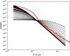 |
Fig. C.1 Power spectrum changing with the iterations. The thick dashed line is the initial guess, the bulge of black lines is where the algorithm converges. The thick solid red line is the power spectrum of the logarithmic Galaxy model with medium fluctuations. The power spectrum is in arbitrary units. |
In Fig. C.2 we show the convergence of the propagated distance variance (Eq. (20)) of a random selection of ten data points. The behavior seen in this plot is qualitatively the same for all data points we investigated. Most data points clearly reach convergence rather quickly, but there are also outliers. In this plot, the lowest line exhibits a kink after it had seemingly already converged. This behavior is unfortunately not entirely suppressible, but it appears to have very little effect on the resulting map because only a small fraction of data points shows this behavior.
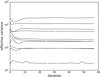 |
Fig. C.2 Propagated distance variance of ten data points changing with the iterations. The
units of the variances are |

In Figs. C.3 and C.4 we show the convergence of the profile functions, where we shifted the functions by a global value to line them up at β( | z | = 0) and α(r = 0). We note that the functions α and β are degenerate with respect to a global addition in their effect on the Galactic profile field and degenerate with the monopole of s as well. This is why a shift by a constant for plotting purposes is reasonable. The z-profile function β seems to reach a fixed point for | z | < 2400 pc. For higher | z | the profile function reaches no clear fixed point. However, for the Galactic profile, where the profile function is exponentiated, this makes only a small difference, since β is already three e-foldings below its values at | z | = 0. The radial profile function α seems to only correct the initial guess mildly, and it is not clear whether the result is independent of the initial guess. However, it appears that α does reach a fixed point.
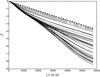 |
Fig. C.3 z-profile function of log ne changing with the iterations. The thick dashed line is the initial guess. |
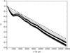 |
Fig. C.4 Radial profile function of log ne changing with the iterations. The thick dashed line is the initial guess. |
Appendix D: Goodness of fit (χ2) of the reconstructions
In this section, we discuss the goodness of fit characterized by the reduced
χ2 value,
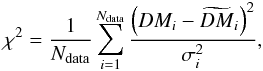 (D.1)where
  is the dispersion data reproduced by
applying the response to our reconstruction,
is the dispersion data reproduced by
applying the response to our reconstruction,
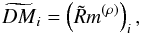 (D.2)and σi is the crudely
propagated distance uncertainty given by
(D.2)and σi is the crudely
propagated distance uncertainty given by
![\appendix \setcounter{section}{4} \begin{eqnarray} \sigma_i = \frac{\sqrt{\mathrm{Var}[d_i]}}{d_i} DM_i. \end{eqnarray}](/articles/aa/full_html/2016/06/aa26717-15/aa26717-15-eq227.png) (D.3)
(D.3)
To set the χ2 value into perspective, we compared them with the χ2 values of the null model (m(ρ) = 0) and the Galactic profile alone (m(ρ) = Δ) The reduced χ2 values corresponding to the maps shown in Fig. 5 are shown in Table D.1. The reconstruction of the mixed data set has a reduced χ2 of 1.31. In Table D.2 we show the reduced χ2 values of the maps shown in Fig. 7. For the reconstruction of the contrast-enhanced input model shown in Fig. 8 the reduced χ2 value is 345 for the null model, 110 for the profile alone, and 2.6 for the full reconstruction.
It is evident from the tables that our reconstructions account for a large part of the data variance in all cases. The Galactic profile without local fluctuations also accounts for a large part of the variance, especially if the distance uncertainties are high and the fluctuation strength of the input model is weak. For our reconstructions the χ2 values are close to 1 for the 25% and 15% data sets. Therefore, we assume that our inference mechanism resolved the most relevant information in the data sets and that the prior assumptions are not too restrictive for these data sets. For the 5% reconstructions the χ2 values are around 3. This is a hint that the data might contain more information than the reconstruction resolves and that more elaborate prior assumptions might yield a better map. However, how to achieve this is a non-trivial question that we do not aim to answer in this work.
Appendix E: Reconstruction with real power spectrum and profile functions
The posterior map our algorithm finds depends on the prior power spectrum, the effective errors, and the profile functions, all of which are simultaneously estimated from the data. To benchmark the efficiency of this joint estimation, we investigated the case where the real power spectrum and the real profile functions are known, that is, only iterating the effective errors. The resulting map serves as an indicator whether our ansatz with unknown hyper parameters is sensible or if the problem is too unrestricted in this setting. We depict the map resulting from the real hyper parameters in Fig. E.1. The morphology of the result obviously does not change. More of the small-scale structure is resolved, and the intensity of the overdensity between the Sun and the Galactic center, which belongs to the ring the original model, is more pronounced. Consequently, this map has a better reduced χ2 value of 1.95 compared to the value of 2.56 of our map with unknown hyperparameters. But considering the amount of unknowns, this is a satisfactory result. We therefore regard our estimation procedure for the hyper parameters as sensible.
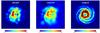 |
Fig. E.1 Top-down view of the reconstructed electron densities in the Galactic plane (in units of cm-3), if we use the real power spectrum and Galactic profile functions (“cheated”), the results from our algorithm (“inferred”), and the original input model. |
Appendix F: Uncertainty map
Here, we discuss the 1σ uncertainty map of reconstructing the Galaxy model with medium fluctuations using the data set with 5000 pulsars and 5% distance uncertainty. We compare the uncertainty map for unknown profile and power spectrum and the uncertainty map for a known profile and power spectrum (see Appendix E) with the corresponding absolute errors. The density maps are shown in Fig. E.1. The uncertainty estimates σ(ρ) (see Eq. (55)) are shown in Fig. F.1. These uncertainties are underestimated because they are calculated from the curvature of the negative log-posterior around its minimum (see Eq. (35)), not from the full distribution. By visual comparison with the absolute error21, | m(ρ) − ρ |, we estimate that the uncertainty estimates are underestimated by a factor of roughly 3. However, their morphology seems to be reliable.
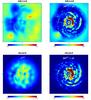 |
Fig. F.1 Top-down view on the Galactic plane, showing the uncertainty estimate (σ(ρ), left panels) and the absolute error (| m(ρ) − ρ|, right panels) for our reconstruction m(ρ) in units of cm-3. The input density ρ has fluctuations of medium strength and is sampled by 5000 pulsars with 5% distance uncertainty. The top row shows the scenario with unknown power spectrum and Galactic profile, the bottom row shows the scenario with known power spectrum and profile. We note that the left and right panels have different color bars. |
Appendix G: Uncertainties of the vertical fall-off
In principle, the posterior variance of α and β is the diagonal of the operator D(ξ) (see Eq. (45)). However, this diagonal is too large because α and β are completely degenerate with respect to a constant shift (α + c and β − c yield the same profile as α and β). This degeneracy yields a large point variance, which is not instructive for quantifying the uncertainty of the vertical fall-off. Therefore, we projected out the eigenvector corresponding to the constant shift before calculating the diagonal of D(ξ). This corrected diagonal is the squared 1σ uncertainty that we plot in Fig. 10.
All Tables
All Figures
|
Fig. 1 Diagram outlining the structure of our modeling. |
| In the text | |
|
Fig. 2 Power spectrum of the NE2001 field without local features, clumps, and voids compared to the three unenhanced Galaxy models. The thick solid line depicts the NE2001 spectrum, the thin dashed lines depict the spectra of the models with strong, medium, and weak fluctuations (from top to bottom). To calculate the spectra, the density peak in the Galactic center is masked. |
| In the text | |
|
Fig. 3 Positions of the simulated 10 000 pulsars on the sky in Galactic coordinates. |
| In the text | |
|
Fig. 4 Histogram showing the distance uncertainty distribution with respect to the distance from the Sun in the mixed measurement set. |
| In the text | |
|
Fig. 5 Several reconstructions of the Galaxy model with medium strength fluctuations. All panels show top-down views of the electron density in the Galactic plane using a linear color scale in units of cm-3. The panels span 36 000 pc in each dimension. The Sun is located at the white dot depicted in each panel. The rows show reconstructions with distance errors of 25%, 15%, and 5% (from top to bottom). The columns show reconstructions with 1000, 5000, and 10 000 pulsars (from left to right). The layout follows Table 1. The top left panel shows the original input model (modified NE2001). The bottom right panel shows the reconstruction of the mixed measurement set. |
| In the text | |
|
Fig. 6 Recovered Galactic profile in the Galactic plane. Shown is a top-down view the Galaxy as in Fig. 5, but here in logarithmic color scale. The input model had medium strength fluctuations, it was recovered using 5000 pulsars with 5% distance uncertainty (corresponding to the bottom middle panel in Fig. 5). Other fluctuation strengths and data sets would yield a very similar image. |
| In the text | |
|
Fig. 7 Reconstructions of the three Galaxy models with fluctuation strengths using 5000 pulsars. All panels show top-down views of the electron density in the Galactic plane using a linear color scale in units of cm-3. The panels span 36 000 pc in each dimension. The rows show reconstructions with distance errors of 15% and 5% (from top to bottom). Bottom row: original Galaxy models. Columns: reconstructions and original input models (modified NE2001) with weak, medium, and strong fluctuations (from left to right). |
| In the text | |
|
Fig. 8 Input model (left) and reconstruction (right) of the contrast-enhanced Galaxy model using 5000 pulsars with distance uncertainties of 5%. Both panels show top-down views of the electron density in the Galactic plane using a linear color scale in units of cm-3. The panels span 36 000 pc in each dimension. |
| In the text | |
|
Fig. 9 Vertical cut through the same Galactic profile as in Fig. 6. Shown is the slice containing the Sun (white dot) and the Galactic center (middle). The image spans 36 kpc × 12 kpc. The color scale is logarithmic. |
| In the text | |
|
Fig. 10 Recovered z-dependent fall-off in logarithmic units (function β in Eq. (40)), input model with medium strength fluctuations. Top left panel: global z-profile (dashed line) as well as the local z-profile (dotted line). In all other panels the solid line is the recovered z-profile while the global and local z-profile are replotted (in dashed and dotted respectively). The gray areas indicate the 1σ uncertainty around the recovered z-profile. In the bottom left corner of each panel: best fitting exponential scale height (and its 1σ uncertainty for the reconstructions). |
| In the text | |
|
Fig. C.1 Power spectrum changing with the iterations. The thick dashed line is the initial guess, the bulge of black lines is where the algorithm converges. The thick solid red line is the power spectrum of the logarithmic Galaxy model with medium fluctuations. The power spectrum is in arbitrary units. |
| In the text | |
|
Fig. C.2 Propagated distance variance of ten data points changing with the iterations. The
units of the variances are |
| In the text | |
|
Fig. C.3 z-profile function of log ne changing with the iterations. The thick dashed line is the initial guess. |
| In the text | |
|
Fig. C.4 Radial profile function of log ne changing with the iterations. The thick dashed line is the initial guess. |
| In the text | |
|
Fig. E.1 Top-down view of the reconstructed electron densities in the Galactic plane (in units of cm-3), if we use the real power spectrum and Galactic profile functions (“cheated”), the results from our algorithm (“inferred”), and the original input model. |
| In the text | |
|
Fig. F.1 Top-down view on the Galactic plane, showing the uncertainty estimate (σ(ρ), left panels) and the absolute error (| m(ρ) − ρ|, right panels) for our reconstruction m(ρ) in units of cm-3. The input density ρ has fluctuations of medium strength and is sampled by 5000 pulsars with 5% distance uncertainty. The top row shows the scenario with unknown power spectrum and Galactic profile, the bottom row shows the scenario with known power spectrum and profile. We note that the left and right panels have different color bars. |
| In the text | |
Current usage metrics show cumulative count of Article Views (full-text article views including HTML views, PDF and ePub downloads, according to the available data) and Abstracts Views on Vision4Press platform.
Data correspond to usage on the plateform after 2015. The current usage metrics is available 48-96 hours after online publication and is updated daily on week days.
Initial download of the metrics may take a while.