| Issue |
A&A
Volume 589, May 2016
|
|
|---|---|---|
| Article Number | A133 | |
| Number of page(s) | 7 | |
| Section | Planets and planetary systems | |
| DOI | https://doi.org/10.1051/0004-6361/201527610 | |
| Published online | 26 April 2016 | |
Pericenter precession induced by a circumstellar disk on the orbit of massive bodies: comparison between analytical predictions and numerical results
Dipartimento di FisicaUniversity of Padova,
via Marzolo 8, 35131 Padova, Italy
e-mail:
Francesco.Marzari@pd.infn.it
Received: 21 October 2015
Accepted: 18 March 2016
Context. Planetesimals and planets embedded in a circumstellar disk are dynamically perturbed by the disk gravity. It causes an apsidal line precession at a rate that depends on the disk density profile and on the distance of the massive body from the star.
Aims. Different analytical models are exploited to compute the precession rate of the perihelion ϖ̇. We compare them to verify their equivalence, in particular after analytical manipulations performed to derive handy formulas, and test their predictions against numerical models in some selected cases.
Methods. The theoretical precession rates were computed with analytical algorithms found in the literature using the Mathematica symbolic code, while the numerical simulations were performed with the hydrodynamical code FARGO.
Results. For low-mass bodies (planetesimals) the analytical approaches described in Binney & Tremaine (2008, Galactic Dynamics, p. 96), Ward (1981, Icarus, 47, 234), and Silsbee & Rafikov (2015a, ApJ, 798, 71) are equivalent under the same initial conditions for the disk in terms of mass, density profile, and inner and outer borders. They also match the numerical values computed with FARGO away from the outer border of the disk reasonably well. On the other hand, the predictions of the classical Mestel disk (Mestel 1963, MNRAS, 126, 553) for disks with p = 1 significantly depart from the numerical solution for radial distances beyond one-third of the disk extension because of the underlying assumption of the Mestel disk is that the outer disk border is equal to infinity. For massive bodies such as terrestrial and giant planets, the agreement of the analytical approaches is progressively poorer because of the changes in the disk structure that are induced by the planet gravity. For giant planets the precession rate changes sign and is higher than the modulus of the theoretical value by a factor ranging from 1.5 to 1.8. In this case, the correction of the formula proposed by Ward (1981) to account for the presence of a gap is a better approximation, at least in predicting a positive precession rate.
Conclusions. Analytical modeling of the precession rate of massive bodies embedded in a circumstellar disk is accurate for planetesimals and terrestrial planets, but it becomes inaccurate when Jupiter-sized planets are considered. The changes they induce in the disk reverse the precession rate and increase it by more than 50%. This discrepancy can be partly solved by including the effects of a gap in the disk density profile in the analytical equations, as done in Ward (1981).
Key words: planet-disk interactions / planets and satellites: dynamical evolution and stability / protoplanetary disks
© ESO, 2016
1. Introduction
The dynamics of massive bodies embedded in a circumstellar disk can be influenced in different ways by the disk gravity. We focus on the apsidal precession of the orbit forced by an axisymmetric gas disk. It can significantly affect the dynamics of planets that are embedded in the disk by shifting the location of potential commensurabilities between them (Tamayo et al. 2015). It also plays an important role in the secular evolution of planetesimal swarms populating disks in binary star systems, as shown in Marzari et al. (2013), Rafikov (2013a,b, 2015a,b), Silsbee & Rafikov (2015a,b).
Various analytical approaches have been developed to estimate this precession rate. The initial physical assumptions at the base of all these models are equivalent, but they gradually depart from each other in the subsequent way of manipulating the equations and in the approximations adopted to derive a simple handy expression. It is then an interesting task to test whether, after all the developments, these analytical formulations are still equivalent and, in particular, whether they match the precession rates computed with numerical models.
In the simplified situation where the disk density profile declines as r-1, the approximation of the disk potential computed by Mestel (1963), the so-called classical Mestel disk, is often used (Tamayo et al. 2015; Rafikov 2013a). For more general disk profiles where the density declines as r− p, where p can be any value, the more complex approaches of Binney & Tremaine (2008) and Ward (1981) are adopted. The more recent approach of Silsbee & Rafikov (2015a) is possibly more versatile since it also allows modeling eccentric disks that might be produced, for example, by a binary companion.
We test the equivalence of these algorithms by focusing on their final formula for computing the disk force and planetesimal or planet precession rates. We compare them under the same physical conditions, not only for p = 1, but also for p = 3 / 2. We also verify their accuracy against numerical simulations modeling the evolution of low-mass bodies (planetesimals), Earth-like planets, and giant planets performed with the hydrocode FARGO (Masset 2000).
In Sect. 2 we describe the different analytical models used to derive an equation for the disk gravitational potential and its derivative, the force. In Sect. 3 we compare the different expressions for the potential and for the force exerted on a body embedded in the disk with the outcome of a numerical model. In Sect. 4 the various analytical predictions concerning the precession rate  for the two disk-density profiles, p = 1 and p = 3 / 2, are compared to the numerical simulations for massless bodies (planetesimals). In Sect. 5 we describe how the values of depend on the mass of the embedded body by computing the values of the precession rate for massive planets. Finally, we discuss our results in Sect. 6.
2. Different equations for the disk gravitational potential and force
The first step for computing the periastron precession rate of a body embedded in a disk is to derive the potential U of the disk; this is usually performed under the assumption that the disk is razor thin and axisymmetrical. Cylindrical coordinates r and φ are usually adopted because of the intrinsic symmetry of the problem. The potential depends on the disk-density profile, which in two dimensions is usually approximated by the superficial density parametrized as a power law: 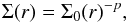 (1)where Σ0 is a reference density value usually given at 1 AU and r is the radial distance along the disk. The density Σ(r) is usually cut off at an inner radius Rin in correspondence to the disk center and at an outer radius Rt beyond which it is assumed to be negligible. Different formulations of U(r,φ) can be found in the literature that we detail below. As a result of the axisymmetrc nature of the problem, the azimuthal angle φ is neglected and we explicitly consider only the radial dependence throughout. All analytical computations were performed with the symbolic code Mathematica1.
2.1. Binney and Tremaine approach: combination of homoemoids
(Binney & Tremaine 2008) computed the potential of an axisymmetric flat disk by adding the potentials of flattened homoemoids (vertical component going to 0) combined to obtain the desired superficial density profiles. The potential in the disk plane is then given by 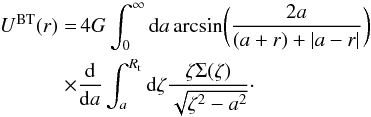 (2)From the potential, the force acting on the disk plane can be deduced. The force is more important since it is used to compute the pericenter precession rate. From deriving the previous expression with respect to the radial distance, the following equation is obtained
 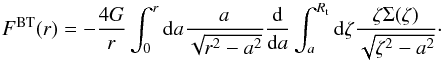 (3)Equation (3) has been rearranged by Tamayo et al. (2015) in the form
 ![\begin{equation} \label{eq:tamaF} F^{\rm BT}(r) =-F_{0}\biggl(\frac{R_{\rm t}}{r}\biggr)^{p}[1+\eta(r,p)] , \end{equation}](/articles/aa/full_html/2016/05/aa27610-15/aa27610-15-eq19.png) (4)where
(4)where 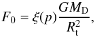 (5)while the terms η and ξ are given by
 ![\begin{equation} \xi(p)=(2-p)\frac{\Gamma\bigl[\frac{2-p}{2}\bigr]\Gamma\bigl[\frac{1+p}{2}\bigr]}{\Gamma\bigl[\frac{3-p}{2}\bigr]\Gamma\bigl[\frac{p}{2}\bigr]} \end{equation}](/articles/aa/full_html/2016/05/aa27610-15/aa27610-15-eq23.png) (6)and
(6)and ![\begin{equation} \eta(r,p)=\frac{2-p}{\pi\xi(p)}\biggl(\frac{R_{\rm t}}{r}\biggr)^{1-p}\left[2K\left(\frac{r^{2}}{R_{\rm t}^{2}}\right)-\pi H\left(p,\frac{r^{2}}{R_{\rm t}^{2}}\right)\right] , \end{equation}](/articles/aa/full_html/2016/05/aa27610-15/aa27610-15-eq24.png) (7)with K the elliptic function of the first kind and H the regularized, generalized hypergeometric function
(7)with K the elliptic function of the first kind and H the regularized, generalized hypergeometric function 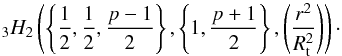 (8)We note that the correction increases as r → Rt but, even if it is normally small, it is still substantial. It is noteworthy that this approach in its original formulation does not consider the possibility of fixing a value for the internal radius of the disk Rin, which is set by default to 0 AU. While this may be a minor limitation when describing young circumstellar disks, it can be a major problem when trying to compute the gravity of a transition disk (Strom et al. 1989) with an internal gap.
2.2. Ward’s approach: superposition of flat rings
(Ward 1981) derived his expression for the potential by superimposing the gravitational potentials of circular flat rings covering the disk and obtained the following formula ![\begin{eqnarray} \label{eq:wardU} U^{\rm W}(r)& = & \, 2\pi G r \Sigma(r)\sum_{k\,=\,0}^{+\infty}A_{k} \biggl[\frac{(4k+1)}{(2k+2-p)(2k-1+p)} \notag \\ &&-\biggl(\frac{1}{2k+2-p}\biggr)\biggl(\frac{R_{\rm in}}{r}\biggr)^{2k+2-p},\\ & -\biggl(\frac{1}{2k-1+p}\biggr)\biggl(\frac{r}{R_{\rm t}}\biggr)^{2k-1+p}\,\biggr] \notag \end{eqnarray}](/articles/aa/full_html/2016/05/aa27610-15/aa27610-15-eq29.png) (9)where Ak = [ (2k) ! / 22k(k ! )2 ] 2. The relative force expression is given by
(9)where Ak = [ (2k) ! / 22k(k ! )2 ] 2. The relative force expression is given by ![\begin{eqnarray} \label{eq:wardF} F^{\rm W}(r)& = & 2\pi G\Sigma(r)\sum_{k=0}^{+\infty}A_{k} \biggl[\frac{(1-p)(4k+1)}{(2k+2-p)(2k-1+p)} \notag \\ &&+\biggl(\frac{2k+1}{2k+2-p}\biggr)\biggl(\frac{R_{\rm in}}{r}\biggr)^{2k+2-p} \\ && -\biggl(\frac{2k}{2k-1+p}\biggr)\biggl(\frac{r}{R_{\rm t}}\biggr)^{2k-1+p}\,\biggr] \notag\cdot \end{eqnarray}](/articles/aa/full_html/2016/05/aa27610-15/aa27610-15-eq31.png) (10)Differently from the model of Binney and Tremaine, in this final equation for the force it is possible to give a value for the inner disk radius Rin.
(10)Differently from the model of Binney and Tremaine, in this final equation for the force it is possible to give a value for the inner disk radius Rin.
The above series developments converge and can be expressed in terms of elliptical and hypergeometric functions. This is done below first for p = 1: 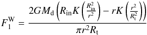 (11)and then for p = 3 / 2:
 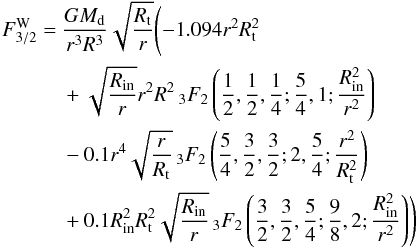 (12)where K is the elliptical integral function of the first kind, while
  is the hypergeometric function.
2.3. Mestel’s classical disk
Mestel (1963) computed the potential of the disk as limit of the potential of a vertically collapsing sphere, an approach that is equivalent to that of Binney & Tremaine (2008). The expression for the force derived by the author is ![\begin{eqnarray} \label{eq:mestF} F^{\rm M}(r)&= &\,-G \biggl(\int_0^r \frac{2\pi \zeta\Sigma(r)}{r^{2}}\,{\rm d}\zeta \notag \\ &&+2\pi\sum_{k=1}^{+\infty}A_{k}\biggl[\frac{2k+1}{r^{2k+2}}\int_0^r \Sigma(r) \zeta^{2k+1}\,{\rm d}\zeta-\Sigma(r)\biggr],\\ &&+2\pi\sum_{k=1}^{+\infty}A_{k}\biggl[\Sigma(r)-2kr^{2k-1}\int_r^{R_{\rm t}} \frac{\Sigma(r)}{\zeta^{2k}}\,{\rm d}\zeta \biggr]\biggr) \notag \end{eqnarray}](/articles/aa/full_html/2016/05/aa27610-15/aa27610-15-eq35.png) (13)which is simplified in Mestel (1963) assuming that
(13)which is simplified in Mestel (1963) assuming that 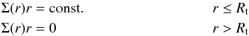 (14)which implies p = 1 in Eq. (1). Under this assumption, the force becomes
 ![\begin{equation} \label{eq:forceMS1} F^{\rm M} (r)=-2\pi G\Sigma(r)\biggl[1+\sum_{k=1}^{+\infty}A_{k}\biggl(\frac{r}{R_{\rm t}}\biggr)^{2k}\, \biggr] . \end{equation}](/articles/aa/full_html/2016/05/aa27610-15/aa27610-15-eq37.png) (15)This last formula is equivalent to Eq. (10)after assuming that Rin = 0 since the term with k = 0 in Eq. (10)gives the constant term equal to 1 in Eq. (15). Finally, the expression for FM is further simplified, assuming that Rt → ∞, into
(15)This last formula is equivalent to Eq. (10)after assuming that Rin = 0 since the term with k = 0 in Eq. (10)gives the constant term equal to 1 in Eq. (15). Finally, the expression for FM is further simplified, assuming that Rt → ∞, into  (16)which is a very simple formula for the force of the classical Mestel passive disk. We call the disk described by Eq. (16) Mestel’s disk.
2.4. Disturbing function of Silsbee and Rafikov
The method adopted in Silsbee & Rafikov (2015a) is similar to that of (Ward 1981), but it has the advantage of also modeling the gravity of eccentric disks. The authors derived the disturbing function on a planetesimal that is due to the disk starting from the gravity of annular components in which the disk can be split. After a series of analytical manipulations, they derive the following expression for the disturbing function, which in our context is the gravitational potential of the disk: ![\begin{equation} U^{\rm SB}=K\left[\int_{\frac{l}{r}}^1 {\rm d}\alpha \, \alpha^{1-p} \, b_{1/2}^{(0)} (\alpha) +\int_{\frac{r}{R}}^1 {\rm d}\alpha \, \alpha^{p-2} \, b_{1/2}^{(0)} (\alpha)\right] , \end{equation}](/articles/aa/full_html/2016/05/aa27610-15/aa27610-15-eq44.png) (17)with
(17)with  the Bessel coefficient (we assume here that the eccentricity of the disk is 0). The function K is defined as
  (18)where Σ0 is the usual constant of the surface density. We assume here that the eccentricity of the disk is 0.
The formulas for the force are equal to Eq. (11)) for p = 1 and Eq. (12)) for p = 3 / 2 as derived from Ward’s formalism. The two approaches are in effect equivalent when they are expressed in terms of elliptical and hypergeometric functions.
3. Comparison between the different analytical equations
The different formulations used to compute the disk force and the precession equations start from the same physical assumptions, but they differ in the subsequent steps performed to reduce the initial complex integrals to more handy equations. These manipulations imply different levels of approximations and may lead to simpler equations whose predictions, however, may not necessarily coincide. We compare the formalisms of Binney & Tremaine (2008), Ward (1981), Mestel (1963), and Silsbee & Rafikov (2015a) under similar conditions of disk mass and profile. However, we must take some basic differences in the final equations of the models into account:
-
The formalisms of Ward (1981) and Silsbee & Rafikov (2015a) allow defining an inner disk radius Rin, while those of Binney & Tremaine (2008) and Mestel (1963) do not.
-
The model of Mestel (1963), in its classical formulation, assumes that the outer disk edge extends to infinity.
-
The equations developed in Ward (1981), Binney & Tremaine (2008), and Silsbee & Rafikov (2015a) can be used with any value of the index p of the disk density profile, while the model of Mestel (1963) can only be applied to the case with p = 1.
When performing the comparison among the different equations, we took these peculiarities of each model into account. The formalisms of Binney & Tremaine (2008) and Mestel (1963) are more limited because they do not allow us to define Rin (and also Rout for Mestel 1963), but it is interesting to test how much these limitations influence the predictive power of these formalisms in terms of force value and pericenter precession rate. For this reason, we compared the different formalisms with a realistic disk model. In principle, the formalism of Binney & Tremaine (2008) could be adapted to model a disk with an inner truncation radius by subtracting from Eq. (4)) the force produced by a small disk extending from the star out to Rin. However, this approach presents some problems. First of all, it would properly work only for p ≤ 2, otherwise the mass of the small inner disk would explode to infinity. This hurdle is not present, for example, in the approach of Ward (1981) since the inner disk is excluded from the force computation, expressed as a series expansion, from the beginning. In addition, the relevant aspect of Eq. (4), as developed by (Tamayo et al. 2015), is the computation of the force through elliptical and hypergeometric functions that allow a straight calculation of the limit of the series expansions. These series converge only slowly, therefore their initial terms are not precise enough to compute the force. The elliptical and hypergeometric functions are defined only within the outer border of the disk (Rt) and not outside, where they give complex values. As a consequence, the force of the inner small disk, to be subtracted from the equation of Binney & Tremaine (2008), needs to be computed in a different way, for example, in that suggested in Krough et al. (1982). Unfortunately, the equation for the force given in Krough et al. (1982) only works for a disk with constant density. This formalism could be integrated to obtain an equation for the force outside a disk with variable density, but it would probably be a more efficient approach to start from the integral of Eq. (3) and include an inner cutoff Rin at that level. All subsequent developments need to be modified to account for Rin, possibly arriving at a final expression similar to that of (Ward 1981). In conclusion, at its present level of development, the formalism of Binney & Tremaine (2008) appears to be less versatile than that of Ward (1981) or Silsbee & Rafikov (2015a).
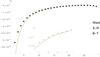 |
Fig. 1 Comparison between the disk force in the three different cases, FBT, FW, and FSR under the assumption that Rin = 0 in the computation of FW, and FSR. The disk-density profile has a p = 1 coefficient. The filled circles are the force values computed numerically with the code FARGO. The enclosed figure shows a more detailed view of the force values near the radial center of the disk. FBT, FW, and FSR are indistinguishable, confirming their equivalence. However, all the analytical estimates do not properly match the numerical solutions close to the star. |
For the comparison between analytical predictions and numerical values, we focused on a standard case with an axisymmetric disk extending out to 30 AU with a density at 1 AU equal to that of the minimum mass solar nebula (Weidenschilling 1977; Hayashi 1981; Desch 2007). Two classical values of the coefficient for the superficial density profile were adopted: p = 1 and p = 3 / 2. The latter will not involve the classical Mestel disk, which requires p = 1. The analytical predictions were also compared to two-dimensional hydrodynamical computations performed with the numerical code FARGO (Masset 2000). In all the simulations we used an evenly spaced grid extending from 0.5 to 30 AU from the star built by 680 rings and 360 sectors. The aspect ratio h = H/r is constant throughout the disk and was set to 0.037 (isothermal simulation). Fourteen massless bodies were embedded in the disk with the initial semimajor axis equally spaced starting from 1 AU out to 29 AU. The initial eccentricity was set to 0.2 so that the pericenter was well defined. We compared the results with an initial eccentricity of 0.1 and observed no significant differences in terms of precession rates. To keep the disk properties constant, an external source of mass was adopted so that mass was refilled at the outer boundary. This is not really an important effect since the time span of the numerical simulation is shorter than the viscous timescale.
In Fig. 1 the value of the force, computed with the three different formalisms FBT, FW, and FSR, is drawn as a function of the radial distance from the star. The comparison is performed assuming that Rin = 0 so that all equations meet the same conditions. They agree well in general, but close to the star they give a poor fit to the numerical values of the force computed with FARGO, possibly because of the Rin = 0 assumption. In a separate plot (Fig. 2) we also show the outcome of the simplified formula of Mestel (1963). It also gives a poor fit in the outer regions of the disk because the condition Rt = ∞ was used to simplify the final equation so the Mestel (1963) model is reliable only in the central part of the disk.
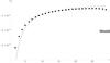 |
Fig. 2 FM computed with the simplified Mestel formula (Eq. (16)), which is most frequently used in common practice. It does not fit the numerical value well close to the star or close to the outer border of the disk. This is due to the assumptions that Rin = 0 and Rout = ∞. |
The situation significantly improves, at least for FW and FSR, when Rin is set to 0.5 AU as in the numerical simulation (see Fig. 3). In this case, the numerical values also match close to the star, and analytical predictions and numerical values agree almost perfectly. This shows that to compute the force, the correction for an inner cutoff Rin is significant. Since all real disks are expected to be truncated at distances of several stellar radii from the star, this appears to be an important aspect in the analytical developments. It may also allow better modeling of transition disks such as those around TW Hya and GM Aur, which show evidences of significant disk clearing out to about 4 AU (Calvet et al. 2002). For p = 3 / 2 the agreement between analytical approaches and numerical values is slightly poorer, as illustrated in Fig. 4. The analytical formulas give somewhat higher values between 5 and 10 AU even if the difference is tiny.
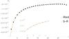 |
Fig. 3 Comparison between the disk force for p = 1 and Rin = 0.5 AU. Both FW and FSR almost perfectly match the numerical values even close to the star, showing the relevance of including an inner cutoff of the disk at Rin. |
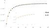 |
Fig. 4 Comparison between the disk force for p = 3 / 2 and Rin = 0.5 AU. FW and FSR now slightly overestimate the numerical values in between 5 and 10 AU from the star. |
In conclusion, the different formulations are in principle equivalent, but after the analytical manipulations performed to derive equations that are more user-friendly, they may differ from each other and from the numerical values computed with the hydrocode FARGO. This applies in particular to the equations derived by Binney & Tremaine (2008) and Mestel (1963).
4. Planetesimal precession rates
The frequency with which the pericenter ϖ of a massive body embedded in the disk precesses as a result of the disk gravitational force can be computed through the following equation, straightforwardly derived from Lagrange’s equations in Murray & Dermott (1999): ![\begin{equation} \frac{\dot{\varpi}}{n}=-\biggl[\frac{F_{\rm D}}{F_{\rm K}}+\frac{1}{2} r\frac{\partial F_{\rm D}/\partial r}{F_{\rm K}}\biggr] , \end{equation}](/articles/aa/full_html/2016/05/aa27610-15/aa27610-15-eq58.png) (19)where FK = GM⋆/r2 is the Keplerian term, M⋆ is the stellar mass, and n is the body mean motion. Into this equation we can insert the different force equations derived in the previous sections (FBT, FW, FM, and FSR) and compare their predictions for the precession rates. This can be done for disks with a power-law index p = 1, while for p = 3 / 2 we can only compare
(19)where FK = GM⋆/r2 is the Keplerian term, M⋆ is the stellar mass, and n is the body mean motion. Into this equation we can insert the different force equations derived in the previous sections (FBT, FW, FM, and FSR) and compare their predictions for the precession rates. This can be done for disks with a power-law index p = 1, while for p = 3 / 2 we can only compare  ,
,  , and
, and  . In this case, we did not test the relevance of the possibility of setting rin = 0.5 AU, as for FW and FSR, but we combined the predictions of all formalisms into a single plot. In short, for the inner radius cannot be set so that Rin = 0 while Rt = 30 AU. When computing and , the inner radius was set to Rin = 0.5 and the outer to Rt = 30 AU, which are the values adopted in the numerical disk model. Finally, for
  the inner and outer cutoffs were set to Rin = 0 and Rt = ∞, respectively. By comparing all the formalisms at once, we can evaluate the relevance of the approximations in the equations of Binney & Tremaine (2008) and Mestel (1963) and verify whether they can be properly used to estimate the correct precession rates.
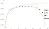 |
Fig. 5 Precession rates for bodies at different distances from the star for a disk-density profile index p = 1. The four analytical values |
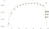 |
Fig. 6 Same as Fig. 5, but with p = 3 / 2. The value of |
Figure 5 shows that for p = 1 both , and almost completely match each other, and they also fit the numerical values well, at least for semimajor axes lower than 20 AU. The approximation Rin = 0 adopted in computing does not significantly influence the precession rate calculation. Beyond 20 AU, the numerical precession rates decline at a lower rate than the analytical predictions and show relevant border effects. The approximations in Mestel’s formula, where the outer border of the disk is pushed to infinity, lead to a behavior of that significantly departs from the numerical values beginning beyond 10 AU, that is, one-third of the disk, and this quickly deteriorates moving farther out in radial distance. is therefore a poor approximation to the real precession rates for most of the disk.
In Fig. 6 the analytical and numerical predictions are compared for p = 3 / 2. In this case, , and appear to be a poorer fit to the numerical data than p = 1 (Fig. 5). Border effects are even stronger in this case, as is shown beyond 25 AU from the star.
From the above results we can conclude that the choice of a different Rin, if small, does not affect the computation of the precession rate significantly, while the choice of pushing the outer border of the disk to infinity is more critical and leads to results significantly different from the numerical ones beginning beyond one-third of the disk. Since the formulas where Rout = ∞ are easier to handle, our computations give a range of validity for their use.
5. Massive planets
A planet embedded in the disk may change the local mass distribution and lead to a different precession rate than is obtained for that of a planetesimal. To test if this is the case, we ran additional simulations with FARGO 4 starting a planet at 10 AU with an initial eccentricity of 0.1. We considered two mass values: m = 5ME and m = 1mJ. The system was evolved for 600 planetary orbits with the planet frozen on its initial orbit to allow the spiral wake to form for the m = 5ME planet and the gap to develop for the Jupiter-sized planet. Then, the planet was released from its initial orbit and further evolved until the eccentricity became about 0.02. Below this value we assumed that the perihelion longitude was not well defined and stopped the simulation. We only have a limited amount of time over which to compute the precession rate because after we release the planet, it starts to migrate and its eccentricity is damped by the disk. However, the initial precession rate is due to the disk mass distribution for the initial orbital elements of the planet, and it can be compared to the analytical predictions.
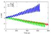 |
Fig. 7 Precession rates for bodies at different distances from the star for a disk-density profile index p = 1. For a giant planet, the precession rate becomes positive even if its modulus is still similar to that of less massive bodies. The modified formula 20 of Ward (1981) that accounts for the presence of a gap in the disk is needed to derive a more accurate analytical prediction. |
In Fig. 7 we compare the perihelion precession rate for the two massive planets and a planetesimal when the coefficient of the disk-density profile is p = 1. The m = 5ME planet shows a precession rate that is similar to that of a planetesimal with a  value only about 15% higher than the predicted value for a test zero-mass body and then higher by approximately the same amount as the theoretical value predicted by the analytical formulas. This implies that the formation of the wake slightly influences the global gravitational attraction of the disk. On the other hand, when we consider a Jupiter-mass planet, the precession rate is not only about 1.8 times higher than the theoretical prediction in modulus, but it also has opposite sign compared to that of a zero-mass body. The gap carved by the planet alters the gravitational pull of the disk, and the precession rate becomes positive and higher in modulus than that of a planetesimal.
A similar behavior is observed when p = 3 / 2, as illustrated in Fig. 8. Even in this case the small planet has  which is approximately 20% higher than the low-mass case (planetesimal), while the of the giant planet is 1.4 higher and of opposite sign. In conclusion, when the theoretical approach is applied to compute the precession rate of a giant planet, care must be taken since the changes in the disk mass distribution that are due to the presence of the planet significantly alter the precession rate.
For giant planets, a better way to compute their precession rate in presence of a gap in the disk is that described by Eqs. (3a) and (3b) in Ward (1981). The potential UW is modified in the following way: ![\begin{eqnarray} \label{eq:wgap} U^{\rm W} &= & 2\pi G\Sigma(r)\!\sum_{k\,=\,0}^{+\infty}A_{k} \biggl[\frac{1}{(2k+2-p)}\biggl(\frac{D_{\rm in}}{r}\biggr)^{2k+2-p}\biggl(1-\biggl(\frac{R_{\rm in}}{D_{\rm in}}\biggr)^{2k+2-p}\biggr) \notag \\ &&+\frac{1}{(2k-1+p)}\biggl(\frac{r}{D_{\rm out}}\biggr)^{2k-1+p}\biggl(1-\biggl(\frac{D_{\rm out}}{R_{\rm t}}\biggr)^{2k-1+p}\biggr)\biggr], \end{eqnarray}](/articles/aa/full_html/2016/05/aa27610-15/aa27610-15-eq78.png) (20)where Din, Dout are the internal and external limits of the gap. To properly use this formula, we first estimated the Din and Dout from the numerical simulations with FARGO and introduced them into Eq. (20). After it is expressed as a function of elliptical and hypergeometrical functions, the potential can be derived to give the force and can be inserted into the equation for the precession rate. In this way, we derived the following values for the precession rates of giant planets orbiting at 10 AU:
(20)where Din, Dout are the internal and external limits of the gap. To properly use this formula, we first estimated the Din and Dout from the numerical simulations with FARGO and introduced them into Eq. (20). After it is expressed as a function of elliptical and hypergeometrical functions, the potential can be derived to give the force and can be inserted into the equation for the precession rate. In this way, we derived the following values for the precession rates of giant planets orbiting at 10 AU:  and
and 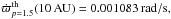 to be compared with
 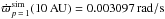 and
and 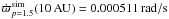 from the numerical simulations. The theoretical values of are positive, in a agreement with the results shown in Figs. 7 and 8, and for a density profile with p = 1, the analytical prediction closely matches the numerical value. For p = 3 / 2 the situation is worse and the theoretical prediction overestimates the numerical value of by almost a factor 2. The shape of the gaps from the numerical simulation does not appear significantly different, and the origin of this larger discrepancy is unclear. However, the analytical predictions appear systematically more inaccurate for p = 3 / 2, also for low-mass bodies such as planetesimals.
For a fully analytical approach for the computation of the precession rate for giant planets that is to be coupled to Ward’s formula, we can use the following approximate equation to computate the gap width derived from Crida et al. (2006): 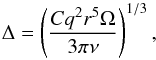 (21)where Δ is the half-width of the gap,
  is the mass ratio, r is the radial distance of the planet, ν is the viscosity, and Ω is the Keplerian frequency of the planet. This equation is derived from Eqs. (1) and (2) of Crida et al. (2006), assuming, as a rough approximation in the torque computations, that r0 = rp and then Ω0 = Ωp and Σ0 = Σp. This equation provided a value of Δ that matches our numerical results well, but as a result of the approximations involved, it must be used with care. More complex and possibly accurate analytical approaches can be found in Crida et al. (2006), Duffell et al. (2013), Kanagawa et al. (2015), Duffell (2015).
6. Discussion and conclusions
We have compared four different analytical equations that are used for computing the precession rate of a body embedded in a circumstellar disk. We found that the equations derived in Binney & Tremaine (2008), Ward (1981) and Silsbee & Rafikov (2015a) agree well for different disk-density profiles and match the numerical results reasonably well. The equations of Binney & Tremaine (2008), Ward (1981) and Silsbee & Rafikov (2015a) are almost equivalent and better match the real values for p = 1 than they do for p = 3 / 2. Only close to the outer border, in particular for p = 3 / 2, all equations lead to some discrepancy with the numerical solution. The classical Mestel disk (Mestel 1963) for p = 1 is a good approximation only in the inner region of the disk. Beyond one-third of the radial extension of the disk, it fails to predict the correct precession rate because of the simplification made in deriving the equation for where Rt was assumed to extend to infinity.
When more massive bodies are considered, the radial density profile of the disk is perturbed at different extents, depending on the mass of the embedded planet. However, for terrestrial planets the equations of Binney & Tremaine (2008), Ward (1981) and Silsbee & Rafikov (2015a) still work reasonably well. On the other hand, for Jupiter-sized planets the precession rate is reversed and higher values are found. This difference can be partly accounted for by using Eqs. (3a) and (3b) of Ward (1981), but they require knowing the size of the gap that is carved by the planet in the disk.If these equations are used, a better match to the numerical values of the precession rate is obtained in particular for p = 1. For p = 3 / 2 the situation is worse since the theoretical value is about twice that computed numerically with FARGO. The scenario in multiplanet systems is expected to be more complex, where each planet, if massive enough, may create a gap that can alter the disk potential acting on another planet member of the system.
Acknowledgments
We thank the anonymous referee for the helpful comments and suggestions.
References
- Binney, J., & Tremaine, S. 2008, Galactic Dynamics, 2nd edn., Princeton Series in Astrophysics (Princeton University Press), 96 [Google Scholar]
- Calvet, N., DAlessio, P., & Hartmann, L. 1992, ApJ, 568, 1008 [Google Scholar]
- Crida, A., Morbidelli, A., & Masset, F. 2006, Icarus 181, 587 [Google Scholar]
- Duffell, P. C. 2015, ApJ 807, L11 [NASA ADS] [CrossRef] [Google Scholar]
- Duffell, P. C., & MacFadyen, A. I. 2013, ApJ 769, 41 [NASA ADS] [CrossRef] [Google Scholar]
- Desch, S. J. 2007, ApJ, 671, 878 [NASA ADS] [CrossRef] [Google Scholar]
- Hayashi, C. 1981, Progr. Theoret. Phys. Suppl., 70, 35 [CrossRef] [Google Scholar]
- Kanagawa, K. D., Muto, T., Tanaka, H., et al. 2015, ApJ, 806, 15 [NASA ADS] [CrossRef] [Google Scholar]
- Krough, F. T., Ng, E. W., & Snyder, W. V. 1982, Celestial Mechanics, 26, 395 [Google Scholar]
- Marzari, F., Thebault, P., Scholl, H., Picogna, G., & Baruteau, C. 2013, A&A, 553, A71 [NASA ADS] [CrossRef] [EDP Sciences] [Google Scholar]
- Masset, F. 2000, A&AS, 141, 165 [NASA ADS] [CrossRef] [EDP Sciences] [Google Scholar]
- Mestel, L. 1963, MNRAS, 126, 553 [NASA ADS] [CrossRef] [Google Scholar]
- Murray, C. D., & Dermott, S. F. 1999, Solar System Dynamics (Cambridge University Press) [Google Scholar]
- Rafikov, R. R. 2013a, ApJ, 765, L8 [NASA ADS] [CrossRef] [Google Scholar]
- Rafikov, R. R. 2013b, ApJ, 764, L16 [NASA ADS] [CrossRef] [Google Scholar]
- Rafikov, R. R., & Silsbee, K. 2015a, ApJ, 798, 69 [NASA ADS] [CrossRef] [Google Scholar]
- Rafikov, R. R., & Silsbee, K. 2015b, ApJ, 798, 70 [NASA ADS] [CrossRef] [Google Scholar]
- Silsbee, K., & Rafikov, R. R. 2015a, ApJ, 798, 71 [NASA ADS] [CrossRef] [Google Scholar]
- Silsbee, K., & Rafikov, R. R. 2015b, ApJ, 808, 58 [NASA ADS] [CrossRef] [Google Scholar]
- Strom, K. M., Strom, S. E., Edwards, S., Cabrit, S., & Skrutskie, M. F. 1989, AJ, 97, 1451 [NASA ADS] [CrossRef] [Google Scholar]
- Tamayo, D., Triaud, A. H. M., Menou, K., & Rein, H. 2015, ApJ, 805, 100 [NASA ADS] [CrossRef] [Google Scholar]
- Ward, W. R. 1981, Icarus, 47, 234 [NASA ADS] [CrossRef] [Google Scholar]
- Weidenschilling, S. J. 1977, Astrophys. Space Sci., 51, 153 [NASA ADS] [CrossRef] [Google Scholar]
All Figures
|
Fig. 1 Comparison between the disk force in the three different cases, FBT, FW, and FSR under the assumption that Rin = 0 in the computation of FW, and FSR. The disk-density profile has a p = 1 coefficient. The filled circles are the force values computed numerically with the code FARGO. The enclosed figure shows a more detailed view of the force values near the radial center of the disk. FBT, FW, and FSR are indistinguishable, confirming their equivalence. However, all the analytical estimates do not properly match the numerical solutions close to the star. |
| In the text | |
|
Fig. 2 FM computed with the simplified Mestel formula (Eq. (16)), which is most frequently used in common practice. It does not fit the numerical value well close to the star or close to the outer border of the disk. This is due to the assumptions that Rin = 0 and Rout = ∞. |
| In the text | |
|
Fig. 3 Comparison between the disk force for p = 1 and Rin = 0.5 AU. Both FW and FSR almost perfectly match the numerical values even close to the star, showing the relevance of including an inner cutoff of the disk at Rin. |
| In the text | |
|
Fig. 4 Comparison between the disk force for p = 3 / 2 and Rin = 0.5 AU. FW and FSR now slightly overestimate the numerical values in between 5 and 10 AU from the star. |
| In the text | |
|
Fig. 5 Precession rates for bodies at different distances from the star for a disk-density profile index p = 1. The four analytical values |
| In the text | |
|
Fig. 6 Same as Fig. 5, but with p = 3 / 2. The value of |
| In the text | |
|
Fig. 7 Precession rates for bodies at different distances from the star for a disk-density profile index p = 1. For a giant planet, the precession rate becomes positive even if its modulus is still similar to that of less massive bodies. The modified formula 20 of Ward (1981) that accounts for the presence of a gap in the disk is needed to derive a more accurate analytical prediction. |
| In the text | |
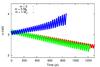 |
Fig. 8 Same as Fig.7, but with p = 3 / 2. |
| In the text | |
Current usage metrics show cumulative count of Article Views (full-text article views including HTML views, PDF and ePub downloads, according to the available data) and Abstracts Views on Vision4Press platform.
Data correspond to usage on the plateform after 2015. The current usage metrics is available 48-96 hours after online publication and is updated daily on week days.
Initial download of the metrics may take a while.