| Issue |
A&A
Volume 589, May 2016
|
|
|---|---|---|
| Article Number | A39 | |
| Number of page(s) | 5 | |
| Section | The Sun | |
| DOI | https://doi.org/10.1051/0004-6361/201527593 | |
| Published online | 12 April 2016 | |
On the interpretation and applicability of κ-distributions
1
Royal Belgian Institute for Space Aeronomy, 3 Avenue Circulaire, 1180
Brussels, Belgium
2
School of Mathematics and Statistics, University of St.
Andrews, St
Andrews, Fife,
KY16 9SS,
UK
3
Institut für Theoretische Physik, Lehrstuhl IV: Weltraum- und
Astrophysik, Ruhr-Universität Bochum, 44780
Bochum,
Germany
e-mail:
This email address is being protected from spambots. You need JavaScript enabled to view it.
4
Research Department of Complex Plasmas, Ruhr-Universität
Bochum, 44780
Bochum,
Germany
5
Institute for Physical Science and Technology, University of
Maryland, College
Park, USA
6
School of Space Research, Kyung Hee University,
Korea
Received: 19 October 2015
Accepted: 6 March 2016
Abstract
Context. The generally accepted representation of κ-distributions in space plasma physics allows for two different alternatives, namely assuming either the temperature or the thermal velocity to be κ-independent.
Aims. The present paper aims to clarify the issue concerning which of the two possible choices and the related physical interpretation is correct.
Methods. A quantitative comparison of the consequences of the use of both distributions for specific physical systems leads to their correct interpretation.
Results. It is found that both alternatives can be realized, but they are valid for principally different physical systems.
Conclusions. The investigation demonstrates that, before employing one of the two alternatives, one should be conscious about the nature of the physical system one intends to describe, otherwise one would possibly obtain unphysical results.
Key words: solar wind / plasmas / instabilities
© ESO, 2016
1. Introduction
The κ-distributions are useful tools for quantitative treatment of nonthermal space and astrophysical plasmas (e.g., Pierrard & Lazar 2010; Livadiotis & McComas 2013; Fahr et al. 2014, and references therein). After their heuristic first definition almost 50 years ago they have not only been used in innumerable applications, but various authors have successfully derived κ-distributions more rigorously for specific physical system. These studies include Hasegawa et al. (1985), who considered a plasma in a prescribed suprathermal radiation field, or Ma & Summers (1998), who assumed the presence of prescribed stationary whistler turbulence. More recent example is Yoon (2014), who self-consistently solved the problem of an electron distribution that is in a dynamic equilibrium with electrostatic Langmuir turbulence. Other authors even attempted to motivate the physical significance of κ-distributions from fundamental principles; these include Tsallis (1988), who considered the generalized version of the Renyi entropy, or Treumann & Jaroschek (2008), who constructed a statistical mechanical theory of such power-law distributions via generalizing Gibbsian theory. Despite these theoretical foundations, there exists as yet no generally accepted unique interpretation of κ-distributions (see Livadiotis 2015, and references therein). As discussed recently in Lazar et al. (2015), one can instead distinguish two principally different alternatives.
The first choice dates back to the original idea for the definition of κ-distributions, which first appeared in printed form in Vasyliunas (1968), but can be traced back to Stanislav Olbert, as acknowledged by the author himself. When Olbert introduced it in one of his own papers published a few months later in the same year, he motivated his definition of κ-distributions in the context of magnetospheric electron spectral measurements as follows (Olbert 1968): “[...] the electron speed distribution [...] is of the form 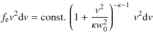 (1)where v is the actual speed, w0 is the most probable speed of electrons, and κ is a “free” parameter whose value is a measure of the departure of the distribution from its Maxwellian character (letting κ approach infinity leads to the Maxwellian distribution). We shall not go into the reasons for this choice except to mention that it seems to be justifiable on the basis of other independent observations”. Evidently, with this ad-hoc definition Olbert (1968) intended to describe an enhanced fraction of suprathermal particles heuristically, as compared to a Maxwellian distribution. Naturally, such suprathermal κ-distribution is characterized by a higher κ-dependent temperature.
Contrary to this expectation Livadiotis (2015) recently offered a different view by stating, “The temperature acquires a physical meaning as soon as the Maxwell’s kinetic definition coincides with the Clausius’s thermodynamic definition [...]. This is the actual temperature of a system; it is unique and independent of the kappa index”.
In order to have a κ-independent temperature, it is easy to see (Sect. 2) that one must consider the thermal velocity (called w0 in Olbert’s definition) to be κ-dependent. A slightly more subtle aspect is another consequence of this assumption; i.e., it not only implies an enhancement of the velocity distribution (VDF) relative to the associated Maxwellian at higher velocities, but also the enhancement of the core population at very low velocities.
The obvious question that arises is: which of the two interpretations is correct or can both be valid for different physical systems? The purpose of the present paper is to answer this question. To this end we define the κ-distributions explicitly in Sect. 2, critically discuss their physical implications in Sects. 3 and 4, and summarize our findings in the concluding Sect. 5.
2. Definitions of the κ-distributions
In most general form, one can define bi-κ-distributions in a magnetized plasma as follows (Lazar et al. 2015): ![Mathematical equation: \begin{eqnarray} F_K (v_{\parallel}, v_{\perp}) & = & {1 \over \pi^{3/2} \theta_{\perp}^2 \theta_{\parallel}} \, {\Gamma(\kappa +1) \over \kappa^{3/2} \Gamma(\kappa -1/2)} \left(1 + {v_{\parallel}^2\over \kappa \theta_{\parallel}^2 } + {v_{\perp}^2\over \kappa \theta_{\perp}^2 }\right)^{-\kappa-1} \nonumber \\ & = & \left[m \over \pi k_{\rm B} (2\kappa-3)\right]^{3/2} {1 \over T^{\rm K}_\perp \sqrt{T^{\rm K}_\parallel}} {\Gamma(\kappa +1) \over \Gamma(\kappa -1/2)} \nonumber\\ &&\quad \times \left[1+ {m \over k_{\rm B} (2\kappa-3)} \left( {v_{\parallel}^2\over T^{\rm K}_{\parallel} } - {v_{\perp}^2\over T^{\rm K}_{\perp} }\right) \right], \label{kappas} \end{eqnarray}](/articles/aa/full_html/2016/05/aa27593-15/aa27593-15-eq5.png) (2)where v∥ and v⊥ denote particle velocity parallel and perpendicular w.r.t. a large-scale magnetic field, T∥ , ⊥ and θ∥ , ⊥ the corresponding temperatures and thermal velocities, which are related by
(2)where v∥ and v⊥ denote particle velocity parallel and perpendicular w.r.t. a large-scale magnetic field, T∥ , ⊥ and θ∥ , ⊥ the corresponding temperatures and thermal velocities, which are related by 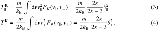 In the above m is particle mass, kB the Boltzmann constant, Γ is the Gamma function, and κ ∈ (3/2,∞ ].
As already pointed out in Lazar et al. (2015), despite this general formulation of the bi-κ-distributions, the interpretation of the temperatures can be ambiguous, as they can be understood and interpreted in two alternative ways:
-
(A)
The temperatures of the bi-κ-distributions and of the associated bi-Maxwellian are identical, i.e.
 . This implies that thermal velocities are κ-dependent via
 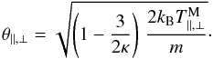 (5)This corresponds to the alternative interpretation advocated by Livadiotis (2015).
 -
(B)
Thermal velocities of bi-κ-distributions and of the associated bi-Maxwellian are identical, i.e.,
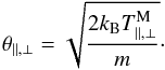 (6)This implies that the temperatures are κ-dependent via
  (7)This corresponds to the original definition by Olbert (1968).
 |
Fig. 1 The two alternative bi-κ-distributions for κ = 9/4 and 2θ⊥/c = θ∥/c = 0.02, and the associated Maxwellian model: panela) displays their parallel cuts and panelsb) and c) show the contours of the full VDFs at the levels (dotted lines) indicated in panela). Evidently both bi-κ-distributions exhibit enhanced tails relative to the Maxwellian but Kappa-A has, in addition, also an enhanced core. |
In the following, we refer to these alternatives as “Kappa-A” and “Kappa-B”, respectively. These κ-distributions differ in a crucial way, as illustrated in Fig. 1, where (a) the parallel part of the two κ-distributions for κ = 9/4 is shown along with the associated Maxwellian; and where (b) contour plots of the VDFs at the level indicated in panel (a) are given. As is evident from panel (a), per construction, both κ-distributions are enhanced at higher velocities relative to the Maxwellian. However, interestingly, Kappa-A additionally exhibits an increased core population. Consequently, unavoidably, a question arises, namely, Which of the two κ-distributions is the correct one? The answer should be found on the basis of quantitative modeling and by considering the consequences of their use for specific physical scenarios. This is discussed in the following section.
3. Comparison of the two κ-distributions
3.1. Non-Maxwellian plasmas due to reduced interactions
One argument for the formation of enhanced suprathermal VDF tails, for example in the solar wind, is the lack of collisions or, more generally, because of insufficient interactions, which could maintain a Maxwellian equilibrium. In this case, it is expected that there should be comparatively more particles with higher velocities, and fewer particles with lower velocities (e.g., Fichtner & Sreenivasan 1993). With a glance at the original purpose, one would prefer Kappa-B for such a scenario: Olbert (1968) intended to describe a particle velocity distribution that has, compared to a Maxwellian, an enhanced fraction of suprathermal particles. Such an enhanced halo of the VDF must be expected to form at the expense of its core population, i.e., one must expect the modified distribution to be depleted at low velocities.
This expectation has been confirmed with the recent direct comparison of using Kappa-A or Kappa-B versus the associated Maxwellian in the studies of plasma waves, and the discussion of the consequences thereof by Lazar et al. (2015). These authors investigated the electromagnetic electron-cyclotron waves driven by perpendicular temperature anisotropy, T⊥/T∥> 1, on the basis of solutions of the corresponding dispersion relation that can be cast into the form 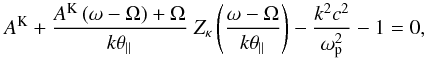 (8)with the temperature anisotropy
  , the complex wave frequency ω(k) = ℜ(ω)(k) + iℑ(ω)(k), the wave number k, the gyrofrequency Ω, the plasma frequency ωp, and the speed of light c. The function
 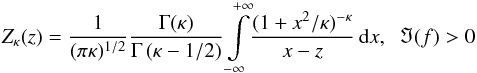 (9)is the modified κ-plasma dispersion function (Lazar et al. 2008). For κ → ∞ one recovers the dispersion relation for a Maxwellian plasma with the standard plasma dispersion function (Fried & Conte 1961).
Lazar et al. (2015) demonstrates that, while all VDFs give very similar dispersion curves, there are significant differences in the growth rates for given anisotropic plasma conditions. One would expect an enhanced fraction of suprathermal particles to increase the growth rates systematically and monotonously, i.e., there should be no wavenumber interval with lower growth rates when compared to the Maxwellian. This behavior is exactly exhibited by Kappa-B. In contrast, the use of Kappa-A results in nonmonotonously higher or lower growth rates than the Maxwellian; an example is provided with Fig. 2.
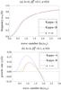 |
Fig. 2 a) Dispersion curves ℜ(ω)(k) and b) growth rates ℑ(ω)(k) derived for a bi-Maxwellian (solid lines), a bi-Kappa-A (dot-dashed lines), and a bi-Kappa-B (dashed lines) for AK,M = 4, a plasma |

Consequently, for a plasma scenario apparently envisaged by Olbert (1968), i.e., a VDF with an enhanced tail rather than an additionally enhanced core, the answer to the above question is that Kappa-B is the correct choice.
3.2. Non-Maxwellian plasmas due to specific wave-particle interactions
It has also been suggested that the high-velocity power-law tails can form as a result of specific wave-particle interactions, e.g., electromagnetic waves (Hasegawa et al. 1985), Whistler waves (Ma & Summers 1998), fast-mode waves (Roberts & Miller 1998), Alfvén waves (Leubner 2000), or stochastic acceleration by turbulence of arbitrary nature but characterized by a diffusion coefficient with an inverse dependence of velocity (Bian et al. 2014). In improvement of such test-particle approaches, Yoon (2014) self-consistently solved the problem of an (isotropic) electron distribution that is in a dynamic equilibrium with electrostatic Langmuir turbulence.
To briefly overview Yoon’s theory, the steady-state isotropic electron VDF F(v) in the presence of Langmuir turbulence intensity  is given by
 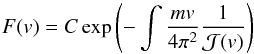 (10)with
 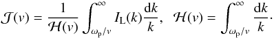 (11)This solution is derived from the particle kinetic equation that describes diffusion and friction (or drag) in velocity space arising from the spontaneously emitted electrostatic Langmuir fluctuations. With
  , where TM is the isotropic Maxwellian temperature, one obtains the Maxwell distribution, FM(v) = Cexp(−mv2/2kBTM). However, Yoon (2014) assumed a generalized Kappa distribution,
 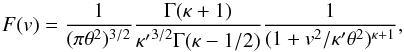 (12)where it should be noted that, unlike the customary κ-model, κ′ is generally allowed to be different from κ. The effective temperature is given by
 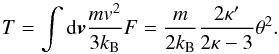 (13)Note that the above definition is essentially the same as Eqs. (3) and (4), except that Eq. (13) defines isotropic temperature and that on the right-hand side of the last equality, the numerator is given by κ′ instead of κ.
Upon comparing the assumed solution (12) and the formal steady-state solution (10), it quickly becomes obvious that the reduced Langmuir fluctuation spectrum  must be given by
 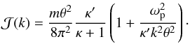 (14)It also follows from the definitions of ℋ and given by Eq. (11) that the full Langmuir intensity can be deduced as
 ![Mathematical equation: \begin{equation} I_{\rm L}(k)=\frac{m\theta^2}{8\pi^2}\frac{\kappa'}{\kappa+1} \left(1+\frac{\omega_{\rm p}^2}{\kappa'k^2\theta^2} \left[1+2{\cal H}(k)\right]\right). \label{IL} \end{equation}](/articles/aa/full_html/2016/05/aa27593-15/aa27593-15-eq49.png) (15)We note that with ℋ = 0 (see the discussion in Yoon 2014) Eqs. (14) and (15) become identical.
(15)We note that with ℋ = 0 (see the discussion in Yoon 2014) Eqs. (14) and (15) become identical.
Yoon (2014) subsequently demonstrated that the solution  for the reduced Langmuir fluctuation spectrum is also, consistently, the steady-state solution of the wave kinetic equation, when exclusively linear wave-particle interactions are considered. Including the nonlinear terms in the wave kinetic equation, Yoon (2014) rederived the exact solution for the full Langmuir intensity as
 ![Mathematical equation: \begin{equation} I_{\rm L}(k)=\frac{k_{\rm B}T_i}{4\pi^2}\left[1+\frac{4}{3} \left(\kappa-\frac{3}{2}\right) \frac{\omega_{\rm p}^2}{\kappa'k^2\theta^2}\right], \label{IL_alt} \end{equation}](/articles/aa/full_html/2016/05/aa27593-15/aa27593-15-eq52.png) (16)which must be identical to Eq. (15). Consequently, it immediately follows that
(16)which must be identical to Eq. (15). Consequently, it immediately follows that 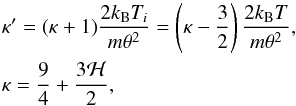 (17)which with ℋ = 0 (see the discussion in Yoon 2014) leads to κ = 9/4.
Consequently, the self-consistent solution can be summarized by a coupled set of solutions,  (18)where κ′ no longer appears. Clearly, the electron VDF is of the type Kappa-A. A noteworthy feature associated with the Langmuir intensity is that the long-wavelength regime (k → 0) is enhanced over the Maxwellian limit, IL(k) = kBTe/ (4π2), while for short wavelengths, the Langmuir fluctuation spectrum decreases relative to the Maxwellian limit. It is the relation (17), particularly the specific identification of κ′ = (2κ−3)kBT/mθ2, which renders Eq. (13) into the θ2 vs. T relationship of the first type, which in turn, led to the Kappa-A model.
As evidenced from Fig. 1, the Kappa-A distribution self-consistently constructed by Yoon (2014) exhibits not only an enhanced high-velocity tail but also an enhanced core population. The latter enhancement can only be understood if a process exists that keeps more particles (relative to the Maxwellian) at low velocities. In the final solution (18), this can be understood in the context of the wave-particle resonance condition, ωp ≃ k·v between the low-velocity electrons and reduced Langmuir fluctuation spectrum in the short-wavelength regime (k ≫ 1). The reduced Langmuir intensity spectrum (relative to the Maxwellian case) leads to an accumulation of low-velocity electrons near v ~ 0, as the wave-particle resonance becomes ineffective, while for high-velocity particles the enhanced Langmuir intensity near k ~ 0 leads to acceleration and, thereby, to the formation of the power-law tail.
Consequently, one can state in general that, if a process exists that keeps more particles (relative to a Maxwellian) at low velocities, the answer to the above question is that Kappa-A is the correct choice: the low-velocity enhancement balances the high-velocity enhancement, so that the temperature is indeed independent of parameter κ.
4. An alternative view: two Maxwellian limits for a given κ-distribution
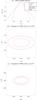 |
Fig. 3 Models of VDFs: bi-Kappa from Eq. (2) with 2θ⊥/c = θ∥/c = 0.02 (dashed blue lines) and κ = 9/4, and bi-Maxwellian limits (κ → ∞) with the same temperature (Maxwellian-H with dash-dotted lines) or with a lower temperature (Maxwellian-C with solid lines). Parallel cuts F(v∥) are shown in panela), and isocontours at 4 × 10⁻³ in panelb) and 10-2 in panelc), corresponding to dotted lines in panela). Notice the difference between the Maxwellian limits. |
We have seen above that not only a κ-model, as in Eq. (2), can be introduced in two different manners with respect to a given Maxwellian limit by considering the temperature to be κ-dependent (Kappa-B) or not (Kappa-A), but also that both κ-VDFs can be realized. The difference in the κ-VDFs signifies a principal difference of the corresponding physical systems.
In practice, i.e., when interpreting measurements, this contrast becomes evident in a different way. Suppose that a set of measurements for a physical system, of which one does not know a priori all properties, can be well-fitted by a κ-distribution Eq. (2). It is now, depending on its interpretation as a Kappa-A or a Kappa-B distribution, possible to consider two Maxwellian limits: namely, a cooler (C) Maxwellian with  , reproducing the low-energy core of the κ-VDF, or a Maxwellian limit with a central peak that is markedly lower but the same temperature as the κ-VDF, i.e.,
  . For illustration, such a κ-VDF and its two Maxwellian limits are shown in Fig. 3.
In this situation the above question can be rephrased: Which of the two Maxwellian distributions is the correct limit? Again the answer depends on the properties of (or physical processes realized in) the considered physical system. Relative to the Maxwellian-C the κ-distribution shows enhanced high-velocity tails and a somewhat reduced core, and, therefore this distribution function of type Kappa-B. This may enable two distinct applications, namely, either to extract the effects of the suprathermal particles by comparison to the Maxwellian core (e.g., dissipation and instabilities, as discussed in Lazar et al. 2015) or to model the particle acceleration (Leubner 2000; Bian et al. 2014). Alternatively, relative to the Maxwellian of equal temperature the κ-distribution exhibits both enhanced tails and an enhanced core, and is, thus, of type Kappa-A. This allows us to study processes that lead to an accumulation of particles at low velocities as the process discussed in Sect. 3 above. The relaxation of a Kappa distribution by keeping the temperature constant and reducing only the suprathermal tails (eventually leading to a Maxwellian equilibrium) is also suggested by the
simulations (Vocks & Mann 2003) to be a result of the Coulomb collisions (νc ~ v-3) in the absence of turbulence. This relaxation seems to ensure the escape of suprathermals from the corona if their existence is assumed there.
So, for a correct application, one needs to have an idea about the Maxwellian equilibrium state of the considered system.
5. Conclusions
Interestingly, we find that both alternatives for defining κ-distributions can be correct, but they are valid for different physical systems. Kappa-A describes a system in which a process must exist that enhances the core part of a VDF relative to its Maxwellian counterpart. While this can be the cause of an increased effective collision rate provided by wave-particle interactions, one should expect only specific κ-values to be consistent with a given scenario. Instead, Kappa-B describes a system, where only a high-velocity enhancement occurs, possibly because of the lack of sufficient (effective) collisions between the particles. Thus, Kappa-B appears to be the less specific case and, thus, should be the more frequently realized alternative. With respect to the two alternative Maxwellian limits of a given κ-distributed data set, it is of significance whether or not an external source of energy has to be taken into account. The latter case would correspond to a Kappa-A and the former to a Kappa-B system. In any case, before employing one of these two representations, one should be conscious about the nature of the physical system one intends to describe to avoid obtaining unphysical results.
Acknowledgments
The authors acknowledge support from the Alexander von Humboldt Foundation, the Visiting International Professor (VIP) Programme of the Research School Plus at the Ruhr-Universität Bochum, and the Deutsche Forschungsgemeinschaft (DFG) via grants FI 706/14-1 and SCHL 201/21-1. P.H.Y. acknowledges the support by the BK21 plus program through the National Research Foundation (NRF) funded by the Ministry of Education of Korea. This project has received funding from the European Union’s Seventh Framework Programme for research, technological development and demonstration under grant agreement SHOCK 284515.
References
- Bian, N. H., Emslie, A. G., Stackhouse, D. J., & Kontar, E. P. 2014, ApJ, 796, 142 [NASA ADS] [CrossRef] [Google Scholar]
- Fahr, H.-J., Fichtner, H., & Scherer, K. 2014, J. Geophys. Res., 119, 7998 [Google Scholar]
- Fichtner, H., & Sreenivasan, S. R. 1993, J. Plasma Phys., 49, 101 [NASA ADS] [CrossRef] [Google Scholar]
- Fried, B. D., & Conte, S. D. 1961, The plasma dispersion function (New York: Academic press) [Google Scholar]
- Hasegawa, A., Mima, K., & Duong-van, M., 1985, Phys. Rev. Lett., 54, 2608 [NASA ADS] [CrossRef] [PubMed] [Google Scholar]
- Lazar, M., Schlickeiser, R., Poedts, S., & Tautz, R. C. 2008, MNRAS, 390, 168 [NASA ADS] [CrossRef] [Google Scholar]
- Lazar, M., Poedts, S., & Fichtner, H. 2015, A&A, 582, A124 [NASA ADS] [CrossRef] [EDP Sciences] [Google Scholar]
- Leubner, M. P. 2000, Planet. Space Sci., 48, 133 [NASA ADS] [CrossRef] [Google Scholar]
- Livadiotis, G. 2015, J. Geophys. Res., 120, 1607 [Google Scholar]
- Livadiotis, G., & McComas, D. J. 2013, Space Sci. Rev., 175, 183 [NASA ADS] [CrossRef] [Google Scholar]
- Ma, C.-y., & Summers, D. 1998, Geophys. Res. Lett., 25, 4099 [NASA ADS] [CrossRef] [Google Scholar]
- Olbert, S. 1968, in Physics of the Magnetosphere, eds. R. D. L. Carovillano, & J. F. McClay, Astrophys. Space Sci. Libr., 10, 641 [Google Scholar]
- Pierrard, V., & Lazar, M. 2010, Sol. Phys., 267, 153 [NASA ADS] [CrossRef] [Google Scholar]
- Roberts, D. A., & Miller, J. A. 1998, Geophys. Res. Lett., 25, 607 [NASA ADS] [CrossRef] [Google Scholar]
- Treumann, R. A., & Jaroschek, C. H. 2008, Phys. Rev. Lett., 100, 155005 [NASA ADS] [CrossRef] [PubMed] [Google Scholar]
- Tsallis, C. 1988, J. Stat. Phys., 52, 479 [NASA ADS] [CrossRef] [MathSciNet] [Google Scholar]
- Vasyliunas, V. M. 1968, J. Geophys. Res., 73, 2839 [NASA ADS] [CrossRef] [Google Scholar]
- Vocks, C., & Mann, G. 2003, ApJ, 593, 1134 [NASA ADS] [CrossRef] [Google Scholar]
- Yoon, P. H. 2014, J. Geophys. Res., 119, 7074 [Google Scholar]
All Figures
|
Fig. 1 The two alternative bi-κ-distributions for κ = 9/4 and 2θ⊥/c = θ∥/c = 0.02, and the associated Maxwellian model: panela) displays their parallel cuts and panelsb) and c) show the contours of the full VDFs at the levels (dotted lines) indicated in panela). Evidently both bi-κ-distributions exhibit enhanced tails relative to the Maxwellian but Kappa-A has, in addition, also an enhanced core. |
| In the text | |
|
Fig. 2 a) Dispersion curves ℜ(ω)(k) and b) growth rates ℑ(ω)(k) derived for a bi-Maxwellian (solid lines), a bi-Kappa-A (dot-dashed lines), and a bi-Kappa-B (dashed lines) for AK,M = 4, a plasma |
| In the text | |
|
Fig. 3 Models of VDFs: bi-Kappa from Eq. (2) with 2θ⊥/c = θ∥/c = 0.02 (dashed blue lines) and κ = 9/4, and bi-Maxwellian limits (κ → ∞) with the same temperature (Maxwellian-H with dash-dotted lines) or with a lower temperature (Maxwellian-C with solid lines). Parallel cuts F(v∥) are shown in panela), and isocontours at 4 × 10⁻³ in panelb) and 10-2 in panelc), corresponding to dotted lines in panela). Notice the difference between the Maxwellian limits. |
| In the text | |
Current usage metrics show cumulative count of Article Views (full-text article views including HTML views, PDF and ePub downloads, according to the available data) and Abstracts Views on Vision4Press platform.
Data correspond to usage on the plateform after 2015. The current usage metrics is available 48-96 hours after online publication and is updated daily on week days.
Initial download of the metrics may take a while.