| Issue |
A&A
Volume 588, April 2016
|
|
|---|---|---|
| Article Number | A140 | |
| Number of page(s) | 15 | |
| Section | Numerical methods and codes | |
| DOI | https://doi.org/10.1051/0004-6361/201527724 | |
| Published online | 01 April 2016 | |
SELFI: an object-based, Bayesian method for faint emission line source detection in MUSE deep field data cubes⋆
1 Grenoble Image Parole Signal Automatique, UMR CNRS 5216 – Université de Grenoble, 38400 Saint Martin d’Hères, France
e-mail: This email address is being protected from spambots. You need JavaScript enabled to view it.
2 Centre de Recherche Astrophysique de Lyon, UMR 5574, 9 avenue Charles-André, 69230 Saint Genis Laval, France
Received: 10 November 2015
Accepted: 15 January 2016
Abstract
We present SELFI, the Source Emission Line FInder, a new Bayesian method optimized for detection of faint galaxies in Multi Unit Spectroscopic Explorer (MUSE) deep fields. MUSE is the new panoramic integral field spectrograph at the Very Large Telescope (VLT) that has unique capabilities for spectroscopic investigation of the deep sky. It has provided data cubes with 324 million voxels over a single 1 arcmin2 field of view. To address the challenge of faint-galaxy detection in these large data cubes, we developed a new method that processes 3D data either for modeling or for estimation and extraction of source configurations. This object-based approach yields a natural sparse representation of the sources in massive data fields, such as MUSE data cubes. In the Bayesian framework, the parameters that describe the observed sources are considered random variables. The Bayesian model leads to a general and robust algorithm where the parameters are estimated in a fully data-driven way. This detection algorithm was applied to the MUSE observation of Hubble Deep Field-South. With 27 h total integration time, these observations provide a catalog of 189 sources of various categories and with secured redshift. The algorithm retrieved 91% of the galaxies with only 9% false detection. This method also allowed the discovery of three new Lyα emitters and one [OII] emitter, all without any Hubble Space Telescope counterpart. We analyzed the reasons for failure for some targets, and found that the most important limitation of the method is when faint sources are located in the vicinity of bright spatially resolved galaxies that cannot be approximated by the Sérsic elliptical profile.
Key words: methods: data analysis / methods: statistical
The software and its documentation are available on the MUSE science web service (muse-vlt.eu/science).
© ESO, 2016
1. Introduction
A number of important questions in observational cosmology require large statistical samples of galaxies with measured properties, such as those relating to dark energy or galaxy evolution. With the advent of optical and infrared large telescopes and wide-field imagers, millions of images of high-quality data have been produced in the past 10 years. The number will continue to expand with the new large telescopes and surveys in preparation. For example, the ground-based Large Synoptic Survey Telescope (Ivezic et al. 2008) and the European Space Agency Euclid space mission (Mellier 2012) will each produce petabytes of data of wide-field imaging over the whole sky. Such quantities of data require advanced methods and efficient software dedicated to the automatic search for galaxies in these wide deep field images of the sky. Various tools have been developed during the last decade and have been applied efficiently to these extragalactic fields. The most popular is Source Extractor (SExtractor; Bertin & Arnouts 1996), which has been used for most large surveys, including Hubble Space Telescope (HST) deep imaging.
However, imaging alone does not provide all of the answers in observational cosmology. Spectroscopic information is also required to measure precise redshifts and other important physical information derived from line diagnostics. To date, most spectroscopic observations have been targeted observations using multi-object spectrographs on targets selected from imaging surveys. However, with the start of operation of the Multi Unit Spectroscopic Explorer (MUSE) at the Very Large Telescope (VLT), the context is changing.
MUSE is the new panoramic field spectrograph that was recently commissioned at the VLT (Bacon et al. 2014). It has a field of view of 1 × 1 arcmin2 sampled at 0.2 arcsec, a simultaneous spectral range of 4650 Å to 9300 Å, a spectral resolution of 3000, and the highest throughput of all VLT spectrographs in the optical range. MUSE produces large hyperspectral data cubes of 324 million voxels, corresponding to 300 × 300 × 3600 pixels along the α,δ,λ axes. Its unique capabilities of providing three-dimensional (3D) deep field observations was demonstrated in early observations of Hubble Deep Field-South (HDFS) Bacon et al. (2015), where 27 h of observations were accumulated in this single field. A first analysis of the corresponding data cube led Bacon et al. (2015) to an increase in the number of spectroscopic redshifts already known in this field of an order of magnitude. In addition, 26 very faint (IAB magnitude <30) Lyα emitters without a HST counterpart in the deep broadband imaging were discovered.
As shown by these discoveries, MUSE is particularly sensitive to line emission objects. In the most extreme cases, these galaxies have no detected continuum and thus do not appear in broadband images. The corresponding sources just pop up as a small aggregate in the data cube of a few voxels at low signal-to-noise ratio (S/N). With no a priori information on their location and wavelength, this makes it challenging to find them in the 324 million voxels contained in a single MUSE data cube. Moreover, these faint emission line galaxies co-exist in the deep field with brighter and spatially resolved galaxies at lower redshifts. Sources often appear blended in the broadband images, although they can be clearly distinguished in the data cube owing to their specific spectral signature.
For all of these reasons, it is obvious that detection techniques developed for 2D imaging data cannot deal with the intrinsic 3D information content of data cubes, which means that other methods need to be investigated. Large data cubes in astronomy are not new. Radio telescopes have produced such data cubes for a long time, and thus methods to find sources in these data cubes have been developed. In the recent literature, different source-detection algorithms have been proposed for finding spectral line sources in previous large surveys, including the HI Parkes All-Sky Survey (HIPASS; Meyer et al. 2004), and the Austrian Square Kilometer Array Pathfinder (ASKAP; DeBoer et al. 2009). See Koribalski (2012) and Popping et al. (2012) for overviews on spectral-line source detection. The source-detection method developed for the HIPASS survey is composed of two combined algorithms: MULTIFIND, which is based on a flux threshold approach, and TOPHAT, which consists of applying a top-hat filter in the spectral domain. These two algorithms produce a large catalog of detected sources that must be checked by multistage processing. By removing multiple detections of the same object or spurious detections, the final catalog contains one thirtieth of the sources proposed by MULTIFIND and TOPHAT. The number of false detections produced by the automatic algorithms MUTIFIND and TOPHAT is prohibitive for the MUSE application. Whiting (2012) developed another general source finder, DUCHAMP, for the detection of sources with one low-extended emission line in the 3D data cubes of the ASKAP survey. This algorithm searches areas of the data cube where the emission is above a given flux threshold. DUCHAMP appears to perform for source detection at peak S/N < 3, and a DUCHAMP performance evaluation can be found in Westmeier et al. (2012). We applied DUCHAMP to a MUSE data cube. DUCHAMP was designed for the detection of sources with a single emission line, while the MUSE data cube contains sources with large spectral variability, including a complex continuum with several spectral features. For such sources, DUCHAMP returns as many detected sources as modes in the spectrum, and is thus not appropriate for the MUSE data cube content.
The aim of this study was to develop a new method for galaxy detection in MUSE deep field data cubes. This method needed to be general enough (i.e., using minimal a priori knowledge) to detect all sorts of objects that can be expected in these deep fields, including very faint emission line objects such as Lyα emitters in the HDFS data cube. Our method is based on an object approach that avoids the need to set constraints for merging pixels. A 3D matched filter was first applied to maximize the S/N of the faint emission line galaxies, and a false alarm control criterion for the object proposition was derived. The proposed approach was developed to model the galaxies in spatial and spectral dimensions, and to provide a way to estimate the source configuration from the data. This has led to a fully automatic detection algorithm that needs a few input parameters, such as the desired false alarm probability. The detailed statistical model is described in Meillier et al. (2015b). In this paper we provide the outlines of the method and the astrophysical interpretations of the different steps of the algorithm.
The paper is organized as follows. The problem formulation and the model of the galaxy configuration are described in Sect. 2. The preprocessing steps are detailed in Sect. 3. In Sects. 4 and 5, we present the detection method and the summary of the algorithm. We apply the detection method to the MUSE view of the HDFS and we discuss some strengths and limitations of the approach in Sect. 6.
2. Problem formulation and requirements
Detecting faint and compact emission line galaxies is a complex signal-processing problem that is a combination of estimation and detection. Little a priori information is available on these galaxies, e.g., their location and redshift are not known, nor their shape, light profile, and spectral distribution. Thus we need to implement a strategy to estimate these unknowns. In the following, we detail the choice of the method that was developed to address this challenge.
2.1. Requirements
The proposed method should meet the following requirements:
-
1.
It should have the best possible completion rate, whileproducing a limited number of false detections.
-
2.
Sources are modeled as 3D objects, so the method must be object based.
-
3.
The method should be nonparametric, i.e., it must be able to extract galaxies in large data fields regardless of the number, shape, spectral features, or spatial distribution of the sources.
-
4.
The method should be robust, in case of imperfect input data. Real data are never perfect and often depart from the usual assumption of independent, normal noise properties. The algorithm should be able to cope with such nonideal datasets.
-
5.
The number of input parameters for the algorithm should be limited. When there are too many input parameters, which are possibly not independent, it becomes difficult to explore all of the parameter space. This might bias the result as the user might have to select a given set of parameters a priori.
-
6.
The complete process should be executed in a reasonable computation time.
2.2. Choice of method
Existing methods that have been specifically developed for target detection in hyperspectral images (see Nasrabadi 2014 for a review of hyperspectral target detection methods) are handled pixel-wise and often rely on template matching. Among the few object-based methods in the literature, marked-point processes were examined. These allow the geometry of objects to be detected, the possible relationships between the objects, and the adequacy of the model for the data to be taken into account. This object process depends on parameters that define the model of the sources that are not known and that need to be estimated. The Bayesian approach consists of considering these parameters as random variables. To find the maximum a posteriori estimate, their joint posterior distribution must be written. The Bayes theorem allows the definition of this posterior distribution proportional to a data fidelity term (i.e., the likelihood function) and the prior distribution of the parameters. A crucial point is the compromise between the influence of the chosen priors and the data. If the influence of the priors is too strong, then the posterior distribution gives low importance to the data. A noninformative prior can be chosen to give more influence to the data for the parameter estimation.
2.3. Modeling the galaxy configuration
A point process defined in a 2D space is a random process where its realization is a configuration of points. This can be used to model the spatial distribution of many physical phenomena, including astronomical systems (see Neyman & Scott 1952; Scargle & Babu 2003; and Beisbart et al. 2002, for detailed examples). In our case, the spatial distribution of the galaxies in the two spatial dimensions of the MUSE data cube can be represented by a configuration of points, i.e., it can be interpreted as a realization of a point process. If the points are uniformly distributed in the space, then the point process is said to be homogeneous. In contrast, if the points are mainly located in certain regions of the space, then the process is said to be inhomogeneous, and the function f(·), which is known as the intensity function, describes this probability. Information about the areas that are likely to contain galaxies can be extracted from the data and included in this intensity function. Setting this intensity function is equivalent to defining the regions of the data cube where we will favor the search for galaxies.
If the point process represents the spatial distribution of the galaxies in the data, we need to add some information to describe the physical characteristics of these galaxies (e.g., shape, spectrum, intensity). The marked-point process is an extension of the point process that associates with each point a list of marks that transform a point into an object. These marks can be geometric, to describe the shape of the objects, or parametric, to model the intensity of the galaxies.
We needed a simple model that fits the majority of the observed galaxies to solve the estimation problem. An elliptical shape with a Sérsic profile (Sersic 1963) was used to fit the surface brightness profiles. A Sérsic profile is a general model for the decrease in intensity of the galaxies. Peng et al. (2002) provided a more complex model through their 2D fitting algorithm GALFIT. However, in our case the observed data are deep fields that contain galaxies of relatively small spatial extension.
To define a galaxy as an object ui, the following marks should be added:
-
length of the ellipse axes ai and bi (without differentiating between major and minor axes);
-
orientation of the ellipse θi (the angle between the horizontal and the first axis);
-
index ni of the Sérsic profile, which describes the decrease in intensity
 where α is a scale parameter that depends on the size of the ellipse (and consequently on a and b) to always preserve 95% of the energy of the Sérsic profile in the elliptical support;
 -
spectrum wi, which is evaluated a posteriori from the final estimated configuration.
We note that the model of the galaxy is parametric (as an ellipse for the shape, and a Sérsic profile for the intensity), although the estimation of the parameters a, b, θ, and n is data driven. There is no parametric description for the spectral mark as we have no a priori information concerning the spectral composition of the observed galaxies.
2.4. Observation model and parameter estimation
With the marked-point process, we associate an observation model that explains the data. The data cube is decomposed into the contribution of the galaxy configuration and a random part related to the noise. This noise is the result of measurement noise, sky photon noise, and sky subtraction residuals. The photon noise related to the galaxies is negligible. The noise is also assumed to be spectrally independent; only source contributions are convolved by the point spread function (PSF). The noise is finally defined as an additive spatially white Gaussian noise where the mean and variance parameters  are unknown and should be estimated for each wavelength λ.
To summarize the estimation problem, the unknown parameters to be estimated are
-
noise parameters:
at each λ; -
object process marks: the number of galaxies n, their positions, their shapes (ai,bi,θi,ni) for 1 ≤ i ≤ n, and their spectra.
The Bayesian approach leads to the optimizing of the posterior density function of these unknown parameters. This function is proportional to the data fidelity term, which is defined by the Gaussian likelihood function deduced from the observation model, and to the priors on the unknown parameters. Noninformative priors are used, except for the configuration prior, which includes some hard penalization on the overlapping ratio. This penalization excludes all of the configuration of objects that do not respect the Rayleigh criterion.
3. Preprocessing
3.1. Need for cube preprocessing
As indicated in paragraph 2.3, the intensity function f(·) of the point process can be defined from the data to favor some regions of the cube for the detection of galaxies. We note that the main motivation of this study was the detection of distant emission line galaxies of low spatial extension. The bright extended galaxies and those that contain a continuous spectral component can be easily detected on the white image. The point process used in this paper focuses on the detection of emission line galaxies, although no information on the faintest ones can be extracted from the data without preprocessing as their S/N is very low. We propose defining a preprocessing that increases the S/N of such sources and that provides an intensity function for the point process.
3.2. Matched filter
The optimal filter for increasing the S/N by one signal (here as the 3D response of the galaxies) is the matched filter. The distant emission line galaxies can be seen as 3D point sources before the spreading by the PSF. As the emission line is not exactly a point in the spectral dimension, being a few pixels large, the response of such sources is close to the PSF with a larger spectral component.
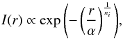
In the case of the MUSE data, the 3D PSF is spatially and spectrally separable; detailed study of this PSF can be found in Serre et al. (2010) and Villeneuve et al. (2011). We use here a simplified model of the 3D PSF where both the spatial and the spectral components of the PSF are considered spatially invariant but change with the wavelength. Consequently, the spatial component of the matched filter is a 3D data cube where each frame is the spatial response of the MUSE instrument at a given wavelength. The spectral component is summarized in a matrix where each column contains the spectral response of the MUSE instrument at the considered wavelength. We note that it has been artificially enlarged to take into account the spectral width of an emission line. The performance of this matched filter is illustrated in Fig. 1.
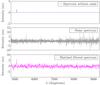 |
Fig. 1 Impact of the matched filter on the spectrum of a simulated faint emission line galaxy (top) embedded in Gaussian noise with a variance on the order of the object intensity. The result of the matched filter (bottom) highlights the emission line that is completely invisible in the noisy version of the spectrum (middle). |
This filtering is applied to the data cube to highlight the presence of 3D signatures that are close to the PSF. We now need a detector that automatically decides whether each spectrum considered belongs to an emission line galaxy. We note that even if the matched filter is designed for emission line galaxies of low extension, other galaxies with powerful enough signatures will not be penalized too much.
3.3. Max-test
The detector is based on a binary hypothesis testing procedure that is applied to each spectrum of the data cube. Before the matched filter, two cases can be distinguished:  Under the null hypothesis, the considered spectrum contains only noise. Under the alternative, an object is located at this position on at least a few consecutive spectral bands. As illustrated in Fig. 1, the principal characteristics of emission line galaxies are highlighted by the matched filter. Consequently, to decide between the two assumptions, we will test the maximum value of the filtered spectrum. This test is called the max-test, and refers to the work of Arias-Castro et al. (2011),
  (1)where Yf(p,q) is the filtered spectrum at position (p,q), and
  is its λth component. The threshold value η(pFA) depends on the false-alarm probability defined for the max-test. To set this threshold value we need to know the distribution of the test under the null hypothesis. The 3D correlation introduced by the matched filtering leads to a nontractable expression of the test under the null hypothesis. If the statistical noise distribution is symmetric and zero-mean, under the null hypothesis the distribution of the maximum value can be deduced from the distribution of the minimum value, for two reasons:
-
they are the same, except their signs;
-
because the source contributions are positive, the minimum value is not contaminated by the galaxies.
Figure 2 shows the empirical probability density and the cumulative density function of the max-test under the null hypothesis. The empirically probability density of the maximum value is obtained from the minimum value of the matched filter spectra (it can be seen as a normalized histogram) because the noise distribution is symmetric. The cumulative distribution function is derived from this probability density function. We note that if the noise distribution is perfectly known, a Monte Carlo sampling of the maximum value of a noise spectrum can be used to derive the probability density and the corresponding cumulative distribution function. The minimum distribution is a good approximation of the statistical distribution of the test T (Eq. (1)) under the null hypothesis. This method is nonparametric, so no assumption is made about the distribution of data other than the symmetry of the noise before the filtering, which has a certain advantage compared to other estimation methods. It also has the advantage of taking into account the 3D correlation (spatial and spectral) of the data, which come from the interpolation process (see Sect. 6.2).
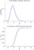 |
Fig. 2 Empirical probability density p(T | ℋ0) of the max-test under the null hypothesis (top) and its cumulative density function (bottom), which is also equal to 1−pFA, where pFA is the false-alarm probability. The variable T represents the values that can be taken by the max-test under the ℋ0 hypothesis. |
We note that the empirical distribution is obtained under stationarity of the noise assumption, so for this preprocessing we need to normalize each band of the data cube at the same mean and variance values. An estimate of the variance is provided with the MUSE data, and an estimate of the noise mean value at each wavelength can be obtained by performing a σ-clipping analysis. If the estimate of the noise variance is not available with the data cube, it can also be obtained by the σ-clipping analysis. The procedure that results from the matched filter and the max-test leads to the same results obtained by the constrained likelihood ratio approach developed by Paris et al. (2013).
3.4. The proposition map
Applying the max-test to the whole cube finally produces a binary map where the pixels can be separated into a class of noisy pixels and a class of pixels that probably belong to a galaxy, with a false-alarm probability pFA. Typically, there are three classes: class  contains each pixel that is lower than the test statistics threshold, i.e., the class of the noisy pixels; the other pixels are in class
  , except for the local maxima, which are in class
  . Only pixels in class are proposed to be at the center of the observed galaxies. Moving the accepted centers into class is accepted, but not into class .
The intensity function f(·) of the point process that models the distribution of the galaxy centers is defined as a step function that can be represented as a 2D map, referred to as the “proposition map” in the following. Figure 3 is an example of a proposition map calculated for a data cube that contains 50 bright sources. During the object proposition process, only white pixels are proposed to be galaxy centers. A black pixel cannot contain an object center.
The object centers are proposed during the birth moves according to this intensity measure, by drawing (1) a pixel uniformly selected in this class; and (2) the continuous position uniformly distributed over the pixel. This way of proposing galaxy centers can be interpreted as a type of super-resolution since it is not limited to the pixel grid.
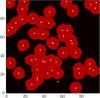 |
Fig. 3 Classification of the pixels according to the max-test for a false-alarm probability pFA = 0.5%. Black pixels belong to class |
3.5. Benefits and risks induced by the proposition map
There are two benefits provided by using this proposition map in the detection process: first, it reduces the number of object configurations to explore and consequently the computation time, and second, the map provides the first error control criterion for each proposed center position of each object. The probability of making an error is limited by the false-alarm probability pFA set by the user. For the case presented in Fig. 3, the white pixels obtained by applying the matched filter and the max-test correspond exactly to the centers of the 50 synthetic objects placed in the data cube, except for one at position (54,12), which is typically a false alarm. The posterior density function to be optimized does not include regularization of the galaxy intensities. This preprocessing step replaces it by favoring the proposition of objects in the most probable areas.
In return, the proposition map does not allow source detection in the areas belonging to noise class . This can lead to missed detection, in particular for the very faint galaxies. A compromise between the number of false alarms and the detection power must be set according to the application considered.
3.6. Additional information provided by the max-test
Further information provided by the max-test includes the location of the emission line in the spectrum:  (2)Assuming that a galaxy has a uniform spectral response over its spatial support, the support of the galaxy should be found in the map produced by the argmax-test. In the case of partially superimposed galaxies, the large spectral variability of the observed sources is expected to be strong enough to make the separation between the two objects possible. In Fig. 4, all 50 objects have the same S/N and, providing that the overlapping ratio respects the Rayleigh criterion, the contributions of two close galaxies are visible on the argmax map. Currently, the spectral information provided by this map is only used to locate the maximum value of the spectrum, i.e., the location of the possible emission line.
 |
Fig. 4 Spectral information on the location of the maximum value of each spectrum of the simulated data cube. |
4. Detection method
4.1. Bayesian model
Given the observation model in which the observations are decomposed into the galaxy contribution and the Gaussian additive noise, the likelihood function can be written as a function of many unknown parameters. In the Bayesian approach, we define an augmented optimization objective that incorporates the prior distributions over the unknown parameters that must be estimated. This objective function is the joint posterior distribution of the unknown parameters. The maximum a posteriori estimate of these parameters corresponds to the mode of the posterior distribution.
Interested readers can refer to Meillier et al. (2015b) for a detailed description of the priors, the posterior distribution, and the optimization process.
4.2. Optimization problem
Given the marginalized posterior distribution, we want to estimate the unknown remaining parameters: m, σ2, and X, where m = [m1,··· ,mλ,··· ,mΛ] is the mean of the noise evaluated at each wavelength, ![Mathematical equation: \hbox{$\boldsymbol{\si}^2 = [\sigma^2_1, \cdots, \sigma^2_\lambda, \cdots, \sigma^2_\Lambda]$}](/articles/aa/full_html/2016/04/aa27724-15/aa27724-15-eq51.png) is the variance of the noise, and X is one realization of the marked-point process. From the posterior distribution, the conditional posterior distribution of each noise parameter (m, σ2) can be deduced given the data and the other parameters. These densities are well defined and can be easily sampled by any numerical software. The case for the object configuration is very different, as it is nonparametric (i.e., the number of sources is unknown), and an estimate cannot be analytically extracted from the posterior distribution. We need to use a sampling algorithm to generate samples and to construct a sample distribution that mimics the posterior distribution of all of these unknown parameters. To address this point, Green (1995) proposed the reversible jump Monte Carlo by Markov chain (RJMCMC) algorithm that answers the variable dimension problem. For our case, two kinds of samplers are implemented in the iterative RJMCMC algorithm: the Gibbs sampler proposed by Geman & Geman (1984) for parameters that have a well-defined conditional posterior density and the Metropolis-Hastings-Green sampler proposed by Green (1995) for the object configuration.
is the variance of the noise, and X is one realization of the marked-point process. From the posterior distribution, the conditional posterior distribution of each noise parameter (m, σ2) can be deduced given the data and the other parameters. These densities are well defined and can be easily sampled by any numerical software. The case for the object configuration is very different, as it is nonparametric (i.e., the number of sources is unknown), and an estimate cannot be analytically extracted from the posterior distribution. We need to use a sampling algorithm to generate samples and to construct a sample distribution that mimics the posterior distribution of all of these unknown parameters. To address this point, Green (1995) proposed the reversible jump Monte Carlo by Markov chain (RJMCMC) algorithm that answers the variable dimension problem. For our case, two kinds of samplers are implemented in the iterative RJMCMC algorithm: the Gibbs sampler proposed by Geman & Geman (1984) for parameters that have a well-defined conditional posterior density and the Metropolis-Hastings-Green sampler proposed by Green (1995) for the object configuration.
4.3. Sampling scheme
The principle of the RJMCMC sampling procedure is based on the construction of a Markov chain of a set of parameters, here m, σ2, and X, which will evolve iteratively by proposing a perturbation to one or more elements of the chain. This perturbation, called “move” in this paper, can be directly accepted (Gibbs sampler) or can go through an acceptance-rejection step (the Metropolis-Hastings-Green sampler). The block diagram of one iteration is shown in Fig. 5, where m∗, σ2∗, and X∗ refer to the proposed values of the different parameters. Figure 5 illustrates the conditional dependence of the parameters:
-
if the object configuration is modified (i.e., a new realization of themarked-point process is generated), the noise parameters are setto their current values, m and σ2, and the impact of the modification X∗ is evaluated with these values;
-
if the modification concerns the noise parameters, their new values are sampled conditional to the unchanged configuration X.
We note that the posterior density is evaluated at each iteration.
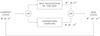 |
Fig. 5 Iterative procedure of the RJMCMC algorithm. The current state is represented by m, σ2, and X, whereas m∗, σ2∗, and X∗ refer to the modified state. |
When the object configuration is modified, i.e., a new realization of the marked-point process is sampled, three different modifications can occur:
-
an object can be added to the current configuration (birth move);
-
an object of the current configuration can be deleted (death move);
-
an object of the current configuration can be modified.
An illustration of the different modifications that can be applied to an object of the current configuration is given in Fig. 6. Details of the birth, death, and modification moves can be found in Appendices A.1−A.3.
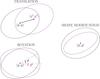 |
Fig. 6 Illustration of the geometric modifications (in violet) that can be applied to one object of the current configuration (in black). |
 |
Fig. 7 Structure of the detection process. The detection block refers to the RJMCMC iterative process described in Fig. 5, and the preprocessing block is detailed in Fig. 8. The two entries LSF and FSF refer to the line-spread function and the field-spread function, which are the spectral and spatial components of the MUSE point-spread function. |
4.4. Estimation of the object configuration
There is no theoretical property to set the number of RJMCMC iterations and to determine the convergence of such an algorithm. In our case, the number of RJMCMC iterations is automatically calibrated according to the evolution of the rates of birth and death moves. If no more birth and death moves are accepted by the iterative procedure during 5000 iterations, then we consider that the algorithm converges to an acceptable solution. As the posterior density is evaluated at each iteration, the selection of the configuration that corresponds to the maximum a posteriori estimate is easy. We let kmax be the iteration index of the maximum value of the posterior distribution. Then the  element of the Markov chains { m } k, { σ2 } k, and { X } k are extracted as the maximum a posteriori estimates.
5. Summary of the algorithm
5.1. Algorithm structure
The main part of the detection is based on the RJMCMC iterative algorithm described in the previous subsection. Its main limitation is its execution time, which strongly depends on the size of the dataset and the number of objects to be detected. To reduce this time, two parallel preprocessing steps were added to the method; the first aims to speed up the detection by initializing the configuration of objects with the most obvious galaxies in the data cube and the second is designed to favor the proposition of objects in the most probable areas of the data cube. The first preprocessing step will be described and illustrated in Sect. 6.3 and the preprocessing for the full data is detailed in Sect. 3.
The intensity function of the marked-point process used to model the configuration of galaxies is based on the max-test (Sect. 3), which highlights the presence of emission line galaxies, although the observations show large spectral variability between the objects detected. For the stars located in the field of view and the galaxies where the spectrum is composed of a continuum, the matched filter and the max-test are not well adapted. The detection of these bright objects can be performed on the white image (see Sect. 6.3). In the current version of the algorithm, we wanted to still use the marked-point process to perform the detection of these very bright galaxies. This allows, in particular, uniform modeling of the galaxies to be preserved regardless of their spectral characteristics. Other source detection methods might be considered to be used directly on the white image (e.g., SExtractor; Bertin & Arnouts 1996), provided that they return a spatial intensity profile for each detected object.
Finally the global structure of the algorithm is presented in Fig. 7. The algorithm inputs are the data cube, the associated variance cube, the false-alarm probability, and the minimum and maximum values for the ellipse axes. We note that the false-alarm probability and the lengths of the ellipse axes are the only parameters set by the user, because they depend on the application and the observation field considered. The size of the observed galaxies is not the same if there are only distant galaxies, or if close galaxies are located in the field of view. The PSF and the white images are evaluated directly from the data cube. Finally, the output of the algorithm is a catalog of detected galaxies with their locations and estimated parameters (i.e., full width at half maximum, Sérsic index, detected on white image or not, position of the emission line).
5.2. Implementation
SELFI has been coded as a Python package. The SELFI package uses the following packages: AstroPy1, NumPy2, and SciPy3. AstroPy was used for FITS file handling and the world coordinate system; NumPy for array-object manipulation, linear algebra, and random number operations; and SciPy for special functions, convolution, norm computation, and image preprocessing.
SELFI has been designed with a multi-object approach. The process starts with the ingestion of the MUSE data cube fits file in a Python cube object, which gives access to the data and variance NumPy arrays, and the associated world coordinate system. Then, all of the preprocessing steps (i.e., S/N, whitening, matched filtering computation) are developed as methods that use and create new cube objects. To minimize CPU time when feasible, the data cube is processed in parallel as a set of monochromatic images that are sent to subprocessors. At each preprocessing step, the user can save the resulting cube objects as FITS files and check them with a data cube viewer.
The minimization algorithm is split up into several Python classes to manage the a posteriori density function, Sérsic objects, Bayesian model, and MCMC iterative process. The process can be initialized from a 3D cube, and also from a 2D image, e.g., with the source detection in the white light image4. The minimization code makes heavy use of numpy array manipulation without looking at the world coordinates. This returns a list of Python source objects. A source object contains the input parameters, the location of the source in degrees, an image of the ellipse Sérsic profile, and the integrated spectrum of the detected source. It can be saved as a FITS file. The process can also use a list of source objects as input and be rerun.
6. Application to the MUSE HDFS field
In the following, we present application of the method to the MUSE HDFS observations. These observations have the advantage that they are very deep and they benefit from high-resolution deep HST images that provide documented catalogs of sources in the HDFS field. These catalogs are used to assess the detection in the MUSE HDFS field with SELFI. The field contains a variety of sources, from bright stars to very faint Lyα emitters, and is thus representative of typical deep field observations with MUSE.
6.1. MUSE HDFS field
The HDFS observations were performed with the HST in 1998 and reported in Williams et al. (2000). It is one of the deepest fields ever observed in the optical-near infrared wavelength range. The WFPC2 observations Casertano et al. (2000) reached a 10σ limiting AB magnitude in the F606W filter at 28.3, and 27.7 in the F814W filter. The HDFS was observed with the MUSE instrument during the last commissioning run of MUSE in late July 2014. The MUSE observations covered a field of view of ~ 1 × 1 arcmin2, which corresponded to 20% of the total WFPC2 field. A total of 27 h integration was accumulated. The detailed observations and data reduction processes, together with a first census of the field and a source catalog, were published in Bacon et al. (2015). The corresponding catalog and data cube are also available online5.
The HDFS hyperspectral cube contains 326 × 331 spatial pixels (or spaxels) and 3641 spectral planes spanning a wavelength range from 4750 Å to 9300 Å. The data cube is formatted in the astronomical standard FITS format (Hanisch et al. 2001), and contains a primary header and two extensions: the primary header has the world coordinate system information, and the first and second extensions contain the data and their estimated variance arrays, respectively. With a total of nearly 400 million voxels, the HDFS data cube information content is large enough to validate the computing efficiency of the proposed method.
The spatial resolution of the MUSE HDFS observations was derived from the MUSE data cube itself, using the bright star in the field. We used the Moffat approximation given by Bacon et al. (2015). We note that the resolution changes with wavelength, as shown in Fig. 2 of Bacon et al. (2015).
From the HST WFPC2 images catalog of Casertano et al. (2000), a subset of 586 sources was located within the MUSE field of view. An aperture summed spectrum was obtained at the location of each of these HST sources and a visual search for emission or absorption lines was performed. Redshift was then inferred by inspection of the spectrum and line identification. In most cases, a specific feature or line combination (e.g. Lyα asymmetry or [OII] resolved doublet) leads to a redshift with a high confidence level. For more details on source identification and redshift determination, see Sect. 4 of Bacon et al. (2015). A large fraction of these sources were also detected in the MUSE white light image, although only a fraction of them have spectral features (e.g., emission or absorption lines) that allow correct redshift identification. Bacon et al. (2015) obtained secure redshifts for 163 sources. In addition, they found 26 Lyα emitters that were too faint to be detected in the WFPC2 HST broadband images. Most of these emission line only galaxies were detected by visual inspection of the data cube monochromatic planes using the SAOImage DS9 data cube viewer6. This catalog is used later as the reference for the performance analysis of SELFI.
6.2. Preprocessing
Since the publication of Bacon et al. (2015), some improvements in data reduction have resulted in better flat fielding, and subsequently improved sky subtraction. We thus used the latest version (1.24) of the HDFS data cube7, which has fewer systematics and is better matched to source detection.
Owing to the dithering process, the edges of the field are less exposed than the main part. The consequence is that the corresponding variance is much higher there. However, our method assumes that the noise variance is invariant within the field of view in each monochromatic plane. We therefore spatially trimmed the original HDFS cube to remove these low S/N edges. The resulting data cube is 311 × 311 × 3641 in size, which corresponds to a 62.2 × 62.2 arcsec2 field of view. We note that the wavelength range (4750, 9300 Å) was preserved.
Although version 1.24 of the HDFS data cube is better than the original version 1.0 used in Bacon et al. (2015), it still contains low spatial frequency residual systematics that are problematic for the detection algorithm. The presence of these systematics lies in opposition to the noise stationarity assumptions. They might then be detected by SELFI, which would lead to an excess of false alarms.
We then apply the matched filter process to the resulting data cube, as described in Sect. 3.2. First, the variance data cube is used to compute the S/N data cube, which is then whitened to zero mean and unity variance for each wavelength plane using a σ-clipping estimation8. The correctly matched filter is then applied using the spatial and spectral PSF information. A simple model of the spectral PSF based on a step function convolved with a Gaussian was used. We note that this does not take into account the possible small variation within the field of view, but it is accurate enough for its use in the matched filter.
Under the null hypothesis, the matched filter does not change the statistical properties of the resulting data cube, and thus the resulting enhanced S/N data cube should still have zero mean and unity variance. However, this was not the case because of the correlated noise characteristics of the variance estimator used in the pipeline. This is due to the interpolation process that is used to build the regularly sampled data cube at the end of the data-reduction process. We therefore applied another whitening process to this data cube using a σ-clipping estimation of the mean and variance at each wavelength plane. The full preprocessing is detailed in Fig. 8.
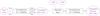 |
Fig. 8 Details of the preprocessing steps, from the original MUSE data to the normalized matched filtered cube. |
As can be seen in Fig. 9, the matched filter data cube now has a much higher S/N than the original dataset. We also note the systematics visible as the low S/N extended signal aligned with the image columns or rows.
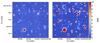 |
Fig. 9 Left: original S/N reconstructed image summed over the 7000 to 7100 Å wavelength range. Right: corresponding match filtered reconstructed white light image. |
6.3. Source detection in the white light image
Given the size of the data cube to explore, the convergence of the algorithm can be prohibitively long. To speed up the process, we first use the algorithm to detect the sources present in the white light image.
The aim of the preprocessing is identical to that presented in the previous section, although it is applied to only one plane instead of the 3641 wavelength layers. For each pixel of the white light image, two cases are considered 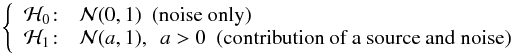 where
where  is the normal density function. The white light image is simply thresholded by testing the validity of the null hypothesis to produce the proposition map: the p-value9 of each pixel of the white light image is evaluated and compared to a level α that corresponds to the desired false alarm probability level. In the case of the white light image, the p-value is evaluated from the normal distribution: under ℋ0,
  . If the p-value is greater than the threshold α then the considered pixel is assumed to be derived from the ℋ0 hypothesis. This is equivalent to comparing the observed value yobs to the threshold η such as
  . With the adopted threshold parameter of η = 3.7, which corresponds to a false-alarm probability of α = 0.001%, a proposition map with 142 candidates is produced (Fig. 10, left panel).
The brightest star in the field is identified for two reasons:
-
its position and its light distribution are known because the spatialPSF was estimated from this star;
-
the Sérsic profile does not fit its Moffat light distribution correctly, which leads to high residuals in the vicinity of the star. To minimize the fitting error, the light distribution of this star is directly fixed to the spatial PSF of the data cube.
The detection algorithm is then launched with the set of parameters given in the Appendix. The process converged after 5029 iterations; a final number of 67 sources were detected (Fig. 10, right panel). The full process took only 8 min on our workstation10. In the next step, these white light detected sources are used as the initial configuration, and their spatial shape and location are fixed to their original values. Only their total spectrum is used in the minimization process.
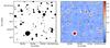 |
Fig. 10 Source detection in the white light image. Left: proposition map. Right: localization of detected sources. Flux units are in 10-20 erg s-1 cm-2. |
6.4. Source detection in the data cube
Similar to the white light detection scheme, the max-test (Sect. 3.3) is used on the matched filtered data cube to provide a list of source candidates. As described in the next section, we used a false-alarm probability of 1.5%, which corresponds to a threshold of 4.1. Here, 178 candidate sources were identified in addition to the 67 white light sources detected previously. The maximum peak emission flux and the corresponding wavelengths derived from the matched filtered data cube are shown in Fig. 11.
The algorithm converged after 9341 iterations and 43 min computing time. A total of 245 sources were detected. We note that of the 1384 birth events proposed by the algorithm, only 178 were accepted. The localization of the detected sources is shown in Fig. 13.
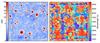 |
Fig. 11 Information maps to illustrate the detection process in the data cube. Left: maximum map obtained by taking the peak flux for each spectrum of the matched filtered data cube. Right: peak wavelengths map. Candidate areas are colored according to the wavelength of their emission peak. |
6.5. Fine tuning of the detection parameters
The probability of false alarms used as the input of the algorithm was defined as a probability of false detection by spaxel, and there is no formal way to match this probability with the source false-detection probability. We also note that this probability is only valid within the model assumption. For example, while the model assumes a symmetric noise distribution, the data cube still suffers from some systematics and is partly correlated.
To select the value of the threshold that allows the detection of as many sources as possible while at the same time limiting the number of false detections, we ran the source detection in the cube with a range of input threshold parameters. As shown in Fig. 12, the number of detections increased almost linearly when the threshold η was decreased from 5 to 4, or equivalently the false-alarm probability pFA increased from 0.1% to 3%. Below η = 4 or above pFA = 3%, the number of detections increased exponentially. At a threshold value of η of 3.4, nearly 500 sources were detected, although most of them were false detections clustered around regions of higher systematics in the data cube. In the particular case of the HDFS data, we empirically selected a threshold value of 4.1 for the detailed detection analysis of the source, because we have a known source catalog that allows us to determine the quality of the detection performed by SELFI. The correspondence between the threshold value and the false-alarm probability for the max-test (Eq. (1)) is obtained from the distribution of the minimum value of each spectrum (see paragraph 3.3). This value of 4.1 corresponds to a false-alarm probability of 1.5% for the max-test applied to the HDFS data. This threshold value should not be used naively for other data cubes; it is preferable to set the false-alarm probability and then to evaluate the corresponding threshold value from the estimated max-test distribution.
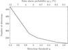 |
Fig. 12 Number of source detections found by the algorithm as a function of the false-alarm probability, or the equivalent of the input threshold parameter. |
6.6. Analysis of the detection results
Using source location, we cross matched the resulting catalog with the reference catalog of Bacon et al. (2015) using a search radius of 1 arcsec. This lead to the following results:
-
From the 189 objects of the reference catalog with secure redshiftidentified in the MUSE data cube sources, 163 were found bySELFI (green markers in Fig. 13), while 26 weremissed (red markers in Fig. 13). This gives asuccess rate of 86%.
-
There were 53 additional sources found by SELFI that match the locations of the HST source catalog Casertano et al. (2000) (white markers in Fig. 13).
-
There were 29 sources detected by SELFI that cannot be matched with MUSE or HST sources (blue markers in Fig. 13).
We first investigated the 26 sources with secured redshift in the reference catalog that were missed by the algorithm. This analysis reveals a mix of causes that led to the failure of detection. Three sources in the reference catalog were probably spurious detections and are not yet present in the used version (1.24) of the data cube. Three sources were faint continuum galaxies that were identified through their absorption lines. One galaxy was truncated by the edge of the field. Seven galaxies were blended with another source at MUSE spatial resolution, but were identified as a different source owing to the HST high-resolution images and their spectral signature. Five galaxies were missed by SELFI because they were located too close to a bright object, although they were not blended. The seven remaining sources all had a low S/N and were probably missed because of the detection threshold selected.
If we remove the spurious detections from the original catalog and leave out the three galaxies detected only by their continuum, the one truncated at the edge of the field of view, and the seven galaxies too blended at MUSE spatial resolution, we are left with five sources that were not found because of the proximity of a bright object, and seven low S/N galaxies. This now gives a success rate of 91%.
We also investigated each of the 29 candidate sources and sorted them between spurious and real detections. Among these candidates, most of them (21) were false detections, and four were galaxies with complex morphology that were split into two sources by the algorithm. Four new sources were identified: three potential Lyα emitters at redshifts 3.1, 3.4 (Fig. 15), and 5.2, and one faint [OII] emitter was also found (Fig. 14). We note that all four of the new detected objects have no HST counterpart. With 21 false detections over a total of 245 sources, SELFI achieves a 9% false-detection rate.
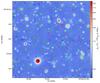 |
Fig. 13 Localization and identification of sources overlaid on the MUSE white light image. Matched sources with secured redshifts (green circles) and HST (white circles) in the reference catalog. New candidate sources (blue circles) and missed sources from the reference catalog (red circles). |
6.7. Performance of the algorithm
With a success rate and a false-detection rate of 91% and 9%, respectively, with respect to the reference catalog, SELFI achieves an overall good performance on this dataset. There are, however, a number of limitations to the algorithm that arise from the analysis of the results.
With only ~40% of the 586 HST sources detected, SELFI does not perform very well in continuum source detection. We note that a fraction of these sources are either too faint to be visible in the MUSE white light image or are blended at MUSE spatial resolution. However, as shown in Fig. 13, a number of sources clearly visible in the MUSE white light image were not detected. This could have been solved by lowering the detection threshold, although this would be at the expense of a much higher false-detection rate. The limited performance of SELFI in white light object detection is not considered critical given that other software like SExactror (Bertin & Arnouts 1996) have been optimized for this work.
The failure of the algorithm to detect sources in the vicinity of brighter resolved galaxies is more problematic (e.g., Fig. 16, top panel), and also the splitting of extended sources into a number of smaller sources (e.g., Fig. 16, bottom panel). In these two cases, the problem is clearly related to the Sérsic elliptical source parametrization that was too simplistic to fit the complex morphology of spatially resolved galaxies. When a faint source lies in the vicinity of such an object, the intrinsic error in the source model is strong enough to prevent the detection of the faint source.
We now investigate the SELFI performance in the regime it was developed for, i.e., the detection of emission line galaxies with faint continuum. Restricting our reference catalog to emission line objects with secured redshift and AB F814 magnitude >26 led to a subset of 105 galaxies, including the 26 detected Lyα emitters without HST counterparts. The corresponding success rate of SELFI is then 84% (88 sources) and 88% (23 sources) for the very faint Lyα emitters. In total, SELFI detected 26 faint Lyα emitters without HST counterparts if we include the three new faint Lyα emitters detected by the algorithm.
As can be seen in Figs. 14 and 15, some source centers are not very accurate. There might be different explanations for this phenomenon:
-
The galaxy light profile is modeled by a Sérsic function sampledon the pixel grid. In the case of faint galaxies, their light profile canbe distorted by strong noise at some spectral bands of highvariance. As the estimation of the light profile is carried out on allof the bands, the approximation by a Sérsic function can beinfluenced by the problematic bands.
-
The proximity of a bright poorly modeled extended source might cause translation of neighbor sources to compensate for eventual modeling residues.
-
If the elliptical shape associated with the Sérsic profile is not sufficiently precise (e.g., incorrect ellipticity, orientation error), translation moves can be accepted by the algorithm as an improvement in the data modeling and cause a shift of the center compared to the actual position.
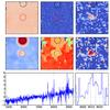 |
Fig. 14 New z = 1.15 [OII]3727 emitter found by the algorithm. Top panels, from left to right: white light, HST F814, and [OII] narrowband images. The image dimension is 5 × 5 arcsec2. Black circle: source location in reference catalog. The bright source at the top is the ID#577 z = 5.8Lyα emitter without a HST counterpart, as already identified in the reference catalog. Red circle: location of a new source. Central panels, from left to right: SELFI max and wavelengths maps (see Sect. 6.4) and [OII] narrowband image derived from the matched filtered data cube. Bottom panels: integrated spectrum, as given by the algorithm. Left: full spectra (smoothed with a Gaussian of 5 pixels FWHM); right: (un-smoothed) zoomed over the [OII] doublet. |
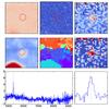 |
Fig. 15 New z = 3.4Lyα emitter found by the algorithm. Red circle: location of a new source. Central panels, from left to right: SELFI max and wavelengths maps (see Sect. 6.4) and Lyα narrowband image derived from the matched filtered data cube. Bottom panels: integrated spectrum, as given by the algorithm. Left: full spectra (smoothed with a Gaussian of 5 pixels FWHM); right: (un-smoothed) zoomed over the Lyα emission line. |
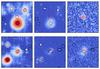 |
Fig. 16 Top panels, from left to right: white light, HST F814, and Lyα narrowband images. Image size is 10 × 10 arcsec2. Black circle: source location in reference catalog. Red circle: location of undetected source. Bottom panels, from left to right: white light, HST F814, and [OII] narrowband images. Black circle: source location in reference catalog. Red circle: location of additional spurious source found by the algorithm. |
7. Conclusions
The SELFI Bayesian method is part of a long-term effort to develop algorithms and software to be used for source detection in MUSE deep field data cubes (Herenz 2015; Cantalupo 2015; Bourguignon et al. 2012; Chatelain et al. 2011; Paris et al. 2011). Given the variety and density of sources found in these fields, we have designed a method that is optimized for the detection of faint compact emission line sources. An important characteristic of the method is that it is source based rather than spectra based. This avoids the difficult and always error-prone part of spectra concatenation of merging the individual spaxel detections into single sources. It also maximizes the signal for the faint sources that otherwise have too low a S/N in an individual spaxel. We also tried to minimize the number of priors and to make the source model as generic as possible. This method then detected all of the different source categories that can be expected in MUSE deep fields.
This method was tested with success on the HDFS MUSE data cube. SELFI retrieved 91% of the sources with secure redshift identified by experts. It must be noted that while most of the identified sources in the reference catalog were based on the HST detection source catalog, SELFI did not make use of this strong prior and worked only on the MUSE data cube. SELFI also detected extremely faint sources (magnitude > 30) with no HST counterpart: 23 of 26 candidate Lyα emitters with no HST counterpart were confirmed by SELFI; in addition, 3 new candidate Lyα emitters were detected. SELFI also detected the first [OII] emitter without a HST counterpart.
Another key performance parameter of the method is the false-detection rate. With only 9% false detections for the HDFS, SELFI performs well. It is not yet possible to use the method blindly, but with such a false-detection rate it becomes manageable to deal with the candidate source checking and validation process.
This method also has some clear limitations. Regarding the data, it assumes that the variance is a function of wavelength, but is also uniform over the field of view. For typical deep field observations, where the sky variance dominates the total variance with respect to the correct variance of the sources, this assumption is perfectly valid. However, for mosaic builds from various exposure times, or dithered exposures that have lower S/N at the edge, like the HDFS, this will no longer be valid and will impose a limit on the data cube for the regions with homogeneous exposure time and/or to process the field in chunks.
The other limitation comes from the elliptical shape and Sérsic profile model, which is good enough for small galaxies, but is not accurate enough to fit the more complex light distribution of extended galaxies. Of course these bright extended galaxies are not the subject of the search performed by SELFI, and it was never intended to provide an accurate fit of their light distribution. However, as seen in Sect. 6.7, in some cases the fitting error prevented the finding of faint sources located in the vicinity of these bright objects. More generally, the method has difficulty with source crowding, as is often the case in deep observations obtained at ground-based spatial resolution. As it is currently designed, SELFI will fail to disentangle low overlapping sources if they are too superimposed, and even if their spectral signatures are very different. Deblending of sources in the MUSE data cube is an important but difficult task. This will need different algorithms and will be the subject of a separate study.
Looking back at the requirements set in Sect. 2.1, we have confirmed the good completion rate (91%) and the low number of false detections (9%). The modeling of the source as a 3D object (requirement 2) was achieved, although its 3D shape is limited to the 2D × 1D distributions. In reality, the spectral profile will change in a galaxy owing to the different composition, kinematics, and state of the gas and the stars. For faint compact sources, however, this approximation is justified. The method is not fully nonparametric (requirement 3) because of the Sérsic model and the elliptical shape of the light distribution, although the number of parameters is limited. More importantly, the nonparametric spectral distribution is preserved in the model. This method was made more robust against imperfect data (requirement 4) by developing advanced preprocessing of the data cube. There are many parameters in the algorithm, but only one key parameter controls the false number (requirement 5). Finally, the full process ran in less than 1 h on a multi-core workstation for the full MUSE data cube (requirement 6).
SELFI was designed to be modular, and two future improvements can already be mentioned. In this first version of SELFI, we chose to model all of the source light profiles using Sérsic functions. Now we see that this is not accurate enough to fit the extended source profiles. The model used for the light distribution of the sources can be easily modified in SELFI code to better fit the source profiles. Another point of improvement is related to the preprocessing of the data that builds the proposition map. In this first version, the map was elaborated according to an individual error control: for each spectrum, we decide if there was only noise or if there was a contribution of a source with respect to a false-alarm probability without taking into account the other detections. In a recent study (Meillier et al. 2015a), we proposed another method that allows the control of a global error criterion: the false-discovery rate in the list of pixels detected. This kind of approach can be developed in parallel with the current preprocessing.
We have made the software and its documentation available on the public MUSE science web service11.
The white light image is derived from the data cube by simple averaging along the wavelength direction.
This data cube or a later version will be available later on the MUSE science web page.
Data are clipped to remove strong artifacts and pixels belonging to sources, and the mean and the variance are estimated from the clipped data. Very faint sources probably remain in the clipped data, but their small contribution compared to the size of the dataset should not affect strongly the estimation of the noise.
The p-value p(yobs) is defined as the probability, under the null hypothesis, of obtaining a value at least equal to the value yobs actually observed: 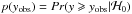 .
.
Workstation 32 cores Intel(R) Xeon(R) CPU E5-4640 0 @ 2.40 GHz and 512 Gb RAM.
Acknowledgments
R. Bacon acknowledges support from the ERC advanced grant 339659-MUSICOS. We would like to thank Johan Richard for his help in testing and validating the method.
References
- Arias-Castro, E., Candès, E. J., Plan, Y., et al. 2011, Annals Stat., 39, 2533 [CrossRef] [Google Scholar]
- Bacon, R., Vernet, J., Borisiva, E., et al. 2014, The Messenger, 157, 13 [NASA ADS] [Google Scholar]
- Bacon, R., Brinchmann, J., Richard, J., et al. 2015, A&A, 575, 75 [Google Scholar]
- Beisbart, C., Kerscher, M., & Mecke, K. 2002, in Morphology of Condensed Matter (Springer), 358 [Google Scholar]
- Bertin, E., & Arnouts, S. 1996, A&AS., 117, 393 [NASA ADS] [CrossRef] [EDP Sciences] [Google Scholar]
- Bourguignon, S., Mary, D., & Slezak, É. 2012, Stat. Methodol., 9, 32 [Google Scholar]
- Cantalupo, S. 2015, in MUSE Consortium Busy week [Google Scholar]
- Casertano, S., de Mello, D., Dickinson, M., et al. 2000, AJ, 120, 2747 [NASA ADS] [CrossRef] [Google Scholar]
- Chatelain, F., Costard, A., & Michel, O. 2011, in Proc. IEEE Int. Conf. Acoustics, Speech and Signal Processing (ICASSP), 3628 [Google Scholar]
- DeBoer, D., Gough, R., Bunton, J., et al. 2009, Proc. IEEE, 97, 1507 [Google Scholar]
- Geman, S., & Geman, D. 1984, IEEE Trans. Pattern Analysis and Machine Intelligence, 721 [Google Scholar]
- Green, P. 1995, Biometrika, 52, 711 [Google Scholar]
- Hanisch, R. J., Farris, A., Greisen, E. W., et al. 2001, A&A, 376, 359 [NASA ADS] [CrossRef] [EDP Sciences] [Google Scholar]
- Herenz, C. 2015, in MUSE Consortium Busy week [Google Scholar]
- Ivezic, Z., Tyson, J., Abel, B., et al. 2008, ArXiv e-print [arXiv:0805.2366] [Google Scholar]
- Koribalski, B. S. 2012, PASA, 29, 359 [NASA ADS] [CrossRef] [Google Scholar]
- Meillier, C., Chatelain, F., Michel, O., & Ayasso, H. 2015a, in Proc. 23rd Europ. Signal Processing Conf. (EUSIPCO 2015) [Google Scholar]
- Meillier, C., Chatelain, F., Michel, O., & Ayasso, H. 2015b, IEEE Trans. Signal Processing, 63, 1911 [NASA ADS] [CrossRef] [Google Scholar]
- Mellier, Y. 2012, in Science from the Next Generation Imaging and Spectroscopic Surveys, EOS Meeting, 1, 3 [Google Scholar]
- Meyer, M. J., Zwaan, M. A., Webster, R. L., et al. 2004, MNRAS, 350, 1195 [NASA ADS] [CrossRef] [Google Scholar]
- Nasrabadi, N. 2014, IEEE Signal Processing Magazine, 31, 34 [NASA ADS] [CrossRef] [Google Scholar]
- Neyman, J., & Scott, E. 1952, ApJ, 116, 144 [NASA ADS] [CrossRef] [Google Scholar]
- Paris, S., Mary, D., Ferrari, A., & Bourguigon, S. 2011, in Proc. 19th Europ. Signal Processing Conf. (EUSIPCO 2011), 1909 [Google Scholar]
- Paris, S., Mary, D., & Ferrari, A. 2013, IEEE Trans. Signal Processing, 61, 1481 [Google Scholar]
- Peng, C. Y., Ho, L. C., Impey, C. D., & Rix, H.-W. 2002, AJ, 124, 266 [NASA ADS] [CrossRef] [Google Scholar]
- Popping, A., Jurek, R., Westmeier, T., et al. 2012, PASA, 29, 318 [NASA ADS] [CrossRef] [Google Scholar]
- Scargle, J. D., & Babu, G. J. 2003, in Handbook of Statistics (Elsevier B.V.), Vol. 21, 795 [Google Scholar]
- Serre, D., Villeneuve, E., Carfantan, H., et al. 2010, in SPIE Conf. Ser., 7736, 773649 [Google Scholar]
- Sersic, J. L. 1963, Bull. Astron. Association of Argentina, 6, 41 [Google Scholar]
- Villeneuve, E., Carfantan, H., & Serre, D. 2011, in Hyperspectral Image and Signal Processing: Evolution in Remote Sensing (WHISPERS), 3rd IEEE Workshop, 1 [Google Scholar]
- Westmeier, T., Popping, A., & Serra, P. 2012, PASA, 29, 276 [NASA ADS] [CrossRef] [Google Scholar]
- Whiting, M. T. 2012, MNRAS, 421, 3242 [NASA ADS] [CrossRef] [Google Scholar]
- Williams, R. E., Baum, S., Bergeron, L. E., et al. 2000, AJ, 120, 2735 [NASA ADS] [CrossRef] [Google Scholar]
Appendix A: RJMCMC algorithm
This Appendix details the different moves used in the RJMCMC sampling of the object configuration.
Appendix A.1: Birth move
The birth move consists of adding a new object to the configuration. This increases the dimensionality of the estimation problem, and consequently the computational complexity of the algorithm. It is of interest to reduce the number of useless propositions, e.g., in areas that contain only background noise. The proposition map built on the same criterion as the marked-point process intensity allows these propositions to be reduced. The birth move consists of a few steps:
-
1.
Selection of a spatial pixel position(pint,qint) on the proposition map (respecting the intensity of the point process). We note that the position of the center is proposed continuously on the pixel grid. The proposed position is obtained by adding a random position
 , then (p,q) = (pint + Δp,qint + Δq).
 -
2.
Proposition of the geometric marks and the Sérsic index according to the uniform priors defined in paragraph 2.3.
-
3.
Addition of the corresponding elliptical object to the current configuration to form the proposition.
-
4.
Acceptance or rejection of the object.
-
5.
Update of the new configuration.
During the third step, if the proposed object does not respect the constraints included in the marked-point process density, such as the overlapping criterion, the birth move is aborted and the configuration remains unchanged (the posterior value is set to the previous one).
Appendix A.2: Death move
The death move consists of deleting an object from the current configuration. This can be useful when an incorrect object has been proposed and accepted because its contribution to the posterior density was sufficiently important at the corresponding
iteration. It can also be accepted in the case of a very faint object where the detection depends on the quality of the noise parameter estimation. The death move is applied using the following procedure:
-
1.
Selection of an object uniformly in the current configuration.
-
2.
Suppression of this object in the proposed configuration.
-
3.
Acceptance or rejection of the object.
-
4.
Update of the new configuration.
We note that if the user selects a very low false-alarm probability, only very bright galaxies can be detected and the proposition map and the intensity of the marked-point process is restricted to areas of the cube that contain strong signals. In this case, the death acceptation rate should be close to 0.
Appendix A.3: Simple modifications of one object
The current configuration can be modified without changing the dimension. A modification to the shape, the position, or the orientation can be applied to one object of the configuration. This allows an object to be changed so that its shape or position best represents the data. The procedure is quite similar to the birth and the death moves:
-
1.
Selection of an object uniformly in the current configuration.
-
2.
Proposition of the new object by applying a uniform distributed modification on the position (translation), the orientation (rotation), or the axis (shape change). When modifying an object, the Sérsic index is systematically sampled according to the uniform distribution defined in paragraph 2.3.
-
3.
Suppression of the selected object in the proposed configuration.
-
4.
Addition of the new object (the modified one).
-
5.
Acceptance or rejection of the object.
-
6.
Update of the new configuration.
The new axis, position, or orientation is uniformly selected in a +/−20% interval around the value of the selected object. Examples of modifications are shown in Fig. 6.
All Figures
|
Fig. 1 Impact of the matched filter on the spectrum of a simulated faint emission line galaxy (top) embedded in Gaussian noise with a variance on the order of the object intensity. The result of the matched filter (bottom) highlights the emission line that is completely invisible in the noisy version of the spectrum (middle). |
| In the text | |
|
Fig. 2 Empirical probability density p(T | ℋ0) of the max-test under the null hypothesis (top) and its cumulative density function (bottom), which is also equal to 1−pFA, where pFA is the false-alarm probability. The variable T represents the values that can be taken by the max-test under the ℋ0 hypothesis. |
| In the text | |
|
Fig. 3 Classification of the pixels according to the max-test for a false-alarm probability pFA = 0.5%. Black pixels belong to class |
| In the text | |
|
Fig. 4 Spectral information on the location of the maximum value of each spectrum of the simulated data cube. |
| In the text | |
|
Fig. 5 Iterative procedure of the RJMCMC algorithm. The current state is represented by m, σ2, and X, whereas m∗, σ2∗, and X∗ refer to the modified state. |
| In the text | |
|
Fig. 6 Illustration of the geometric modifications (in violet) that can be applied to one object of the current configuration (in black). |
| In the text | |
|
Fig. 7 Structure of the detection process. The detection block refers to the RJMCMC iterative process described in Fig. 5, and the preprocessing block is detailed in Fig. 8. The two entries LSF and FSF refer to the line-spread function and the field-spread function, which are the spectral and spatial components of the MUSE point-spread function. |
| In the text | |
|
Fig. 8 Details of the preprocessing steps, from the original MUSE data to the normalized matched filtered cube. |
| In the text | |
|
Fig. 9 Left: original S/N reconstructed image summed over the 7000 to 7100 Å wavelength range. Right: corresponding match filtered reconstructed white light image. |
| In the text | |
|
Fig. 10 Source detection in the white light image. Left: proposition map. Right: localization of detected sources. Flux units are in 10-20 erg s-1 cm-2. |
| In the text | |
|
Fig. 11 Information maps to illustrate the detection process in the data cube. Left: maximum map obtained by taking the peak flux for each spectrum of the matched filtered data cube. Right: peak wavelengths map. Candidate areas are colored according to the wavelength of their emission peak. |
| In the text | |
|
Fig. 12 Number of source detections found by the algorithm as a function of the false-alarm probability, or the equivalent of the input threshold parameter. |
| In the text | |
|
Fig. 13 Localization and identification of sources overlaid on the MUSE white light image. Matched sources with secured redshifts (green circles) and HST (white circles) in the reference catalog. New candidate sources (blue circles) and missed sources from the reference catalog (red circles). |
| In the text | |
|
Fig. 14 New z = 1.15 [OII]3727 emitter found by the algorithm. Top panels, from left to right: white light, HST F814, and [OII] narrowband images. The image dimension is 5 × 5 arcsec2. Black circle: source location in reference catalog. The bright source at the top is the ID#577 z = 5.8Lyα emitter without a HST counterpart, as already identified in the reference catalog. Red circle: location of a new source. Central panels, from left to right: SELFI max and wavelengths maps (see Sect. 6.4) and [OII] narrowband image derived from the matched filtered data cube. Bottom panels: integrated spectrum, as given by the algorithm. Left: full spectra (smoothed with a Gaussian of 5 pixels FWHM); right: (un-smoothed) zoomed over the [OII] doublet. |
| In the text | |
|
Fig. 15 New z = 3.4Lyα emitter found by the algorithm. Red circle: location of a new source. Central panels, from left to right: SELFI max and wavelengths maps (see Sect. 6.4) and Lyα narrowband image derived from the matched filtered data cube. Bottom panels: integrated spectrum, as given by the algorithm. Left: full spectra (smoothed with a Gaussian of 5 pixels FWHM); right: (un-smoothed) zoomed over the Lyα emission line. |
| In the text | |
|
Fig. 16 Top panels, from left to right: white light, HST F814, and Lyα narrowband images. Image size is 10 × 10 arcsec2. Black circle: source location in reference catalog. Red circle: location of undetected source. Bottom panels, from left to right: white light, HST F814, and [OII] narrowband images. Black circle: source location in reference catalog. Red circle: location of additional spurious source found by the algorithm. |
| In the text | |
Current usage metrics show cumulative count of Article Views (full-text article views including HTML views, PDF and ePub downloads, according to the available data) and Abstracts Views on Vision4Press platform.
Data correspond to usage on the plateform after 2015. The current usage metrics is available 48-96 hours after online publication and is updated daily on week days.
Initial download of the metrics may take a while.