| Issue |
A&A
Volume 588, April 2016
|
|
|---|---|---|
| Article Number | A19 | |
| Number of page(s) | 8 | |
| Section | Numerical methods and codes | |
| DOI | https://doi.org/10.1051/0004-6361/201527709 | |
| Published online | 11 March 2016 | |
Frequentist tests for Bayesian models
Astrophysics Group, Blackett Laboratory, Imperial College London,
Prince Consort
Road,
London
SW7 2AZ,
UK
e-mail:
This email address is being protected from spambots. You need JavaScript enabled to view it.
Received: 6 November 2015
Accepted: 1 February 2016
Abstract
Analogues of the frequentist chi-square and F tests are proposed for testing goodness-of-fit and consistency for Bayesian models. Simple examples exhibit these tests’ detection of inconsistency between consecutive experiments with identical parameters, when the first experiment provides the prior for the second. In a related analysis, a quantitative measure is derived for judging the degree of tension between two different experiments with partially overlapping parameter vectors.
Key words: methods: data analysis / methods: statistical
© ESO, 2016
1. Introduction
Bayesian statistical methods are now widely applied in astronomy. Of the new techniques thus introduced, model selection (or comparison) is especially notable in that it replaces the frequentist acceptance-rejection paradigm for testing hypotheses. Thus, given a data set D, there might be several hypotheses { Hk } that have the potential to explain D. From these, Bayesian model selection identifies the particular Hk that best explains D. The procedure is simple, though computationally demanding: starting with an arbitrary pair of the { Hk }, we apply the model selection machinery, discard the weaker hypothesis, replace it with one of the remaining Hk, and repeat.
This procedure usefully disposes of the weakest hypotheses, but there is no guarantee that the surviving Hk explains D. If the correct hypothesis is not included in the { Hk }, we are left with the “best” hypothesis but are not made aware that the search for an explanation should continue. In the context of model selection, the next step would be a comparison of this “best” Hk with the hypothesis that Hk is false. But model selection fails at this point because we cannot compute the required likelihood (Sivia & Skilling 2006, p. 84). Clearly, what is needed is a goodness-of-fit criterion for Bayesian models.
This issue is discussed by Press et al. (2007, p. 779). They note that “There are no good fully Bayesian methods for assessing goodness-of-fit ...” and go on to report that “Sensible Bayesians usually fall back to p-value tail statistics ... when they really need to know if a model is wrong”.
On the assumption that astronomers do really need to know if their models are wrong, this paper adopts a frequentist approach to testing Bayesian models. Although this approach may be immediately abhorrent to committed Bayesians, the role of the tests proposed herein is merely to provide a quantitative measure according to which Bayesians decide whether their models are satisfactory. When they are, the Bayesian inferences are presented – and with increased confidence. When not, flaws in the models or the data must be sought, with the aim of eventually achieving satisfactory Bayesian inferences.
2. Bayesian models
The term Bayesian model – subsequently denoted by ℳ – must now be defined. The natural definition of ℳ is that which must be specified in order that Bayesian inferences can be drawn from D – i.e., in order to compute posterior probabilities. This definition implies that, in addition to the hypothesis H, which introduces the parameter vector α, the prior probability distribution π(α) must also be included in ℳ. Thus, symbolically, we write  (1)It follows that different Bayesian models can share a common H. For example, H may be the hypothesis that D is due to Keplerian motion. But for the motion of a star about the Galaxy’s central black hole, the appropriate π will differ from that for the reflex orbit of star due to a planetary companion.
A further consequence is that a failure of ℳ to explain D is not necessarily due to H: an inappropriate π is also a possibility.
To astronomers accustomed to working only with uniform priors, the notion that a Bayesian model’s poor fit to D could be due to π might be surprising. A specific circumstance where π could be at fault arises when Bayesian methods are used to repeatedly update our knowledge of some phenomenon – e.g., the value of a fundamental constant that over the years is the subject of numerous experiments (X1,...,Xi,...), usually of increasing precision. With an orthodox Bayesian approach, Xi + 1 is analysed with the prior set equal to the posterior from Xi. Thus  (2)This is the classical use of Bayes theorem to update our opinion by incorporating past experience. However, if Xi is flawed – e.g., due to an unrecognized systematic error – then this choice of π impacts negatively on the analysis of Xi + 1, leading perhaps to a poor fit to Di + 1
Now, since subsequent flawless experiments result in the decay of the negative impact of Xi, this recursive procedure is self-correcting, so a Bayesian might argue that the problem can be ignored. But scientists feel obliged to resolve such discrepancies before publishing or undertaking further experiments and therefore need a statistic that quantifies any failure of ℳ to explain D.
3. A goodness-of-fit statistic for Bayesian models
The most widely used goodness-of-fit statistic in the frequentist approach to hypothesis testing is χ2, whose value is determined by the residuals between the fitted model and the data, with no input from prior knowledge. Thus,  (3)is the goodnes-of-fit statistic for the minimum-χ2 solution α0.
A simple analogue of  for Bayesian models is the posterior mean of χ2(α),
  (4)where the posterior distribution
  (5)Here ℒ(α | H,D) is the likelihood of α given data D.
Note that since ⟨ χ2 ⟩ π depends on both constituents of ℳ, namely H and π, it has the potential to detect a poor fit due to either or both being at fault, as required by Sect. 2.
In Eq. (4) the subscript π is attached to ⟨ χ2 ⟩ to stress that a non-trivial, informative prior is included in ℳ. On the other hand, when a uniform prior is assumed, ⟨ χ2 ⟩ is independent of the prior and is then denoted by ⟨ χ2 ⟩ u.
The Bayesian goodness-of-fit statistic ⟨ χ2 ⟩ u is used in Lucy (2014, L14) to illustrate the detection of a weak second orbit in simulations of Gaia scans of an astrometric binary. In that case, H states that the scan residuals are due to the reflex Keplerian orbit caused by one invisible companion. With increasing amplitude of the second orbit, the point comes when the investigator will surely abandon H – i.e., abandon the assumption of just one companion – see Fig. 12, L14.
3.1. p-values
With the classical frequentist acceptance-rejection paradigm, a null hypothesis H0 is rejected on the basis of a p-value tail statistic. Thus, with the χ2 test, H0 is rejected if  , where
  , and accepted otherwise. Here ν = n − k is the number of degrees of freedom, where n is the number of measurements and k is the number of parameters introduced by H0, and β is the designated p-threshold chosen by the investigator.
For a Bayesian model, a p-value can be computed from the ⟨ χ2 ⟩ π statistic, whose approximate distribution is derived below in Sect. 5.1. However, a sharp transition from acceptance to rejection of the null hypothesis at some designated p-value is not recommended. First, p-values overstate the strength of the evidence against H0 (e.g., Sellke et al. 2001). In particular, the value p = 0.05 recommended in elementary texts does not imply strong evidence againts H0. Second, the p-value is best regarded (Sivia & Skilling 2006, p. 85) as serving a qualitative purpose, with a small value prompting us to think about alternative hypotheses. Thus, if ⟨ χ2 ⟩ π exceeds the chosen threshold  , this is a warning that something is amiss and should be investigated, with the degree of concern increasing as β decreases. If the β = 0.001 threshold is exceeded, then the investigator would be well-advised to suspect that ℳ or D is at fault.
Although statistics texts emphasize tests of H not D, astronomers know that D can be corrupted by biases or calibration errors. Departures from normally-distributed errors can also increase ⟨ χ2 ⟩ π.
If D is not at fault, then ℳ is the culprit, implying that either π or H is at fault. If the fault lies with π not H, then we expect that  even though
  .
.
If neither D nor π can be faulted, then the investigator must seek a refined or alternative H.
3.2. Type I and type II errors
In the frequentist approach to hypothesis testing, decision errors are said to be of type I if H is true but the test says reject H, and of type II if H is false but the test says accept H.
Since testing a Bayesian model is not concerned exclusively with H, these definitions must be revised, as follows:
-
A type I error arises when ℳ and D are flawless but the statistic (e.g., ⟨ χ2 ⟩ π) exceeds the designated threshold.
-
A type II error arise when ℳ or D are flawed but the statistic does not exceed the designated threshold.
Here the words accept and reject are avoided. Moreover, no particular threshold is mandatory: it is at the discretion of the investigator and is chosen with regard to the consequences of making a decision error.
4. Statistics of ⟨ χ2 ⟩
The intuitive understanding that scientists have regarding derives from its simplicity and the rigorous theorems on its distribution that allow us to derive confidence regions for multi-dimensional linear models (e.g., Press et al. 2007, Sect. 15.6.4).
Rigorous statistics for χ2 require two assumptions: 1) that the model fitted to D is linear in its parameters; and 2) that measurement errors obey the normal distribution. Nevertheless, even when these standard assumptions do not strictly hold, scientists still commonly rely on to gauge goodness-of-fit, with perhaps Monte Carlo (MC) sampling to provide justification or calibration (e.g., Press et al. 2007, Sect. 15.6.1).
Rigorous results for the statistic ⟨ χ2 ⟩ are therefore of interest. In fact, if we add the assumption of a uniform prior to the above standard assumptions, then we may prove (Appendix A) that  (6)where k is the number of parameters.
Given that Eq. (6) is exact under the stated assumptions, it follows that the quantity ⟨ χ2 ⟩ u − k is distributed as  with ν = n − k degrees of freedom.
For minimum-χ2 fitting of linear models, the solution is always a better fit to D than is the true solution. In particular,  , whereas
  . Accordingly, the + k term in Eq. (6) “corrects” for overfitting and so
  – i.e., the expected value of χ2 for the actual measurement errors.
4.1. Effect of an informative prior
When an informative prior is included in ℳ, an analytic formula for ⟨ χ2 ⟩ π is in general not available. However, its approximate statistical properties are readily found.
Consider again a linear model with normally-distributed errors and suppose further that the experiment (X2) is without flaws. The χ2 surfaces are then self-similar k-dimensional ellipsoids with minimum at α0 ≈ αtrue, the unknown exact solution. Let us now further suppose that the informative prior π(α) derives from a previous flawless experiment (X1). The prior π will then be a convex (bell-shaped) function with maximum at αmax ≈ α0. Now, consider a 1D family of such functions all centred on α0 and ranging from the very broad to the very narrow. For the former ⟨ χ2 ⟩ π ≈ ⟨ χ2 ⟩ u; for the latter  . Thus, ideally, when a Bayesian model ℳ is applied to data D we expect that
  (7)Now, a uniform prior and δ(α − α0) are the limits of the above family of bell-shaped functions. Since the delta function limit is not likely to be closely approached in practice, a first approximation to the distribution of ⟨ χ2 ⟩ π is that of ⟨ χ2 ⟩ u – i.e., that of
  .
.
The above discussion assumes faultless X1 and X2. But now suppose that there is an inconsistency between π and X2. The peak of π at αmax will then in general be offset from the minimum of χ2 at α0. Accordingly, in the calculation of ⟨ χ2 ⟩ π from Eq. (4), the neighbourhood of the χ2 minimum at α0 has reduced weight relative to χ2(αmax) at the peak of π. Evidently, in this circumstance, ⟨ χ2 ⟩ π can greatly exceed ⟨ χ2 ⟩ u, and the investigator is then alerted to the inconsistency.
5. Numerical experiments
Given that rigorous results ⟨ χ2 ⟩ are not available for informative priors, numerical tests are essential to illustrate the discussion of Sect. 4.1.
5.1. A toy model
A simple example with just one parameter μ is as follows: H states that u = μ, and D comprises n measurements ui = μ + σzi, where the zi here and below are independent gaussian variates randomly sampling  . In creating synthetic data, we set μ = 0,σ = 1 and n = 100.
In the first numerical experiment, two independent data sets D1 and D2 are created comprising n1 and n2 measurements, respectively. On the assumption of a uniform prior, the posterior density of μ derived from D1 is  (8)We now regard p(μ | H,D1) as prior knowledge to be taken into account in analysing D2. Thus
  (9)so that the posterior distribution derived from D2 is
  (10)The statistic quantifying the goodness-of-fit achieved when ℳ = { π,H } is applied to data D2 is then
  (11)From N independent data pairs (D1,D2), we obtain N independent values of ⟨ χ2 ⟩ π thus allowing us to test the expectation (Sect. 4.1) that this statistic is approximately distributed as ⟨ χ2 ⟩ u. In Fig. 1, this empirical PDF is plotted together the theoretical PDF for ⟨ χ2 ⟩ u.
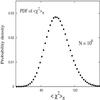 |
Fig. 1 Empirical PDF of ⟨ χ2 ⟩ π derived from the analysis of 106 data pairs D1,D2 as described in Sect. 5.1. The dashed curve is the theoretical PDF for ⟨ χ2 ⟩ u. |
The accuracy of the approximation at large values of χ2 is of special importance. For n = 100 and k = 1, the 0.05,0.01 and 0.001 critical points of ⟨ χ2 ⟩ u are 124.2, 135.6 and 149.2, respectively. From a simulation with N = 106, the number of ⟨ χ2 ⟩ π values exceeding these thresholds are 50 177, 10 011 and 1025, respectively. Thus, the fraction of ⟨ χ2 ⟩ π exceeding the critical values derived from the distribution of ⟨ χ2 ⟩ u are close to their predicted values. Accordingly, the conventional interpretation of these critical values is valid.
In this experiment, the analysis of X2 benefits from knowledge gained from X1. We expect therefore that ⟨ χ2 ⟩ π is less than ⟨ χ2 ⟩ u, since replacing the uniform prior with the informative π obtained from X1 should improve the fit. From 106 repetitions, this proves to be so with probability 0.683. Sampling noise in D1 and D2 accounts for the shortfall.
5.2. Bias test
When X1 and X2 are flawless, the statistic ⟨ χ2 ⟩ π indicates doubts – i.e., type I errors (Sect. 3.2) – about the mutual consistency of X1 and X2 with just the expected frequency. Thus, with the 5% threshold, doubts arise in 5.02% of the above 106 trials. This encourages the use of ⟨ χ2 ⟩ π to detect inconsistency.
Accordingly, in a second test, X1 is flawed due to biased measurements. Thus, now ui = μ + σzi + b for D1. As a result, the prior for X2 obtained from Eq. (9) is compromised, and this impacts on the statistic ⟨ χ2 ⟩ π from Eq. (11).
In Fig. 2, the values of ⟨ χ2 ⟩ π and ⟨ χ2 ⟩ u are plotted against b/σ. Since the compromised prior is excluded from ⟨ χ2 ⟩ u, its values depend only on the flawless data sets D2, and so mostly fall within the (0.05,0.95) interval. In contrast, as b/σ increases, the values of ⟨ χ2 ⟩ π are increasingly affected by the compromised prior.
The mutual consistency of X1 and X2 is assessed on the basis of ⟨ χ2 ⟩ π, with choice of critical level at our discretion. However, when ⟨ χ2 ⟩ π exceeds the 0.1% level at 149.2, we would surely conclude that X1 and X2 are in conflict and seek to resolve the discrepancy. On the other hand, when inconsistency is not indicated, we may accept the Bayesian inferences derived from X2 in the confident belief that incorporating prior knowledge from X1 is justified and beneficial.
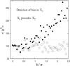 |
Fig. 2 Detection of bias in X1 with the ⟨ χ2 ⟩ π statistic when X2 is analysed with prior derived from X1. Values of ⟨ χ2 ⟩ π (filled circles) and ⟨ χ2 ⟩ u (open circles) are plotted against the bias parameter b/σ. The dashed lines are the 5 and 95% levels. |
This test illustrates the important point that an inappropriate π can corrupt the Bayesian inferences drawn from a flawless experiment. Thus, in this case, the bias in D1 propagates into the posterior p(μ | H,D2) derived from X2. This can be (and is) avoided by preferring the frequentist methodology. But to do so is to forgo the great merit of Bayesian inference, namely its ability to incorporate informative prior information (Feldman & Cousins 1998). If one does therefore prefer Bayesian inference, it is evident that a goodness-of-fit statistic such as ⟨ χ2 ⟩ π is essential in order to detect errors propagating into the posterior distribution from an ill-chosen prior.
5.3. Order reversed
In the above test, the analysis of X2 is preceded by that of X1. This order can be reversed. Thus, with the same N data pairs (D1,D2), we now first analyse X2 with a uniform prior to obtain p(μ | H,D2). This becomes the prior for the analysis of X1. This analysis then gives the posterior p(μ | H,D1) from which a new value of ⟨ χ2 ⟩ π is obtained.
When the values of ⟨ χ2 ⟩ π obtained with this reversed order of analysis are plotted against b/σ, the result is similar to Fig. 2, implying that the order is unimportant. Indeed, statistically, the same decision is reached independently of order. For example, for 105 independent data pairs (D1,D2) with b/σ = 1, the number with ⟨ χ2 ⟩ π> 124.2, the 5% threshold, is 50 267 when X1 precedes X2 and 50 149 when X2 precedes X1.
5.4. Alternative statistic
Noting that the Bayesian evidence is  , the prior-weighted mean of the likelihood, we can, under standard assumptions, write
 ![Mathematical equation: \begin{eqnarray} \bar{ {\cal L}} \propto \exp\left[-\frac{1}{2} \chi^{2}_{\rm eff} \right] \end{eqnarray}](/articles/aa/full_html/2016/04/aa27709-15/aa27709-15-eq102.png) (12)where the effective χ2 (Bridges et al. 2009) is
(12)where the effective χ2 (Bridges et al. 2009) is ![Mathematical equation: \begin{eqnarray} \chi^{2}_{\rm eff} \: = \: - 2 \ln \int \pi(\vec{\alpha}) \exp\left[-\frac{1}{2} \chi^{2}(\vec{\alpha}) \right] {\rm d}V_{\vec{\alpha}}. \end{eqnarray}](/articles/aa/full_html/2016/04/aa27709-15/aa27709-15-eq103.png) (13)This is a possible alternative to ⟨ χ2 ⟩ π defined in Eq. (4). However, in the test of Sect. 5.1, the two values are so nearly identical it is immaterial which mean is used. Here ⟨ χ2 ⟩ π is preferred because it remains well-defined for a uniform prior, for which an analytic result is available (Appendix A).
(13)This is a possible alternative to ⟨ χ2 ⟩ π defined in Eq. (4). However, in the test of Sect. 5.1, the two values are so nearly identical it is immaterial which mean is used. Here ⟨ χ2 ⟩ π is preferred because it remains well-defined for a uniform prior, for which an analytic result is available (Appendix A).
Because ⟨ χ2 ⟩ π and  are nearly identical, the distribution of should approximate that of ⟨ χ2 ⟩ u (Sect. 4.1). To test this, the experiment of Sect. 5.1 is repeated with replacing ⟨ χ2 ⟩ π. From a simulation with N = 106, the number of values exceeding the 0.05, 0.01 and 0.001 thresholds are 50 167, 9951 and 970, respectively. Thus if is chosen as the goodness-of-fit statistic, accurate p-values can be derived on the assumption that
  is distributed as with ν = n − k degrees of freedom. From Sect. 4.1, we expect these p-values to be accurate if π(α) is not more sharply peaked than ℒ(α | H,D).
6. An F statistic for Bayesian models
Inspection of Fig. 2 shows that a more powerful test of inconsistency between X1 and X2 must exist. A systematic displacement of ⟨ χ2 ⟩ π relative to ⟨ χ2 ⟩ u is already evident even when ⟨ χ2 ⟩ π is below the 5% threshold at 124.2. This suggests that a Bayesian analogue of the F statistic be constructed.
6.1. The frequentist F-test
In frequentist statistics, a standard result (e.g., Hamilton 1964, p. 139) in the testing of linear hypotheses is the following: we define the statistic 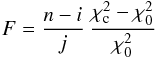 (14)where is the minimum value of χ2 when all i parameters are adjusted, and
  is the minimum value when a linear constraint is imposed on j( ≤ i) parameters, so that only the remaining i − j are adjusted. Then, on the null hypothesis H that the constraint is true, F is distributed as Fν1,ν2 with ν1 = j and ν2 = n − i, where n is the number of measurements. Accordingly, H is tested by comparing the value F given by Eq. (14) with critical values Fν1,ν2,β derived from the distribution of Fν1,ν2.
Note that when j = i, the constraint completely determines α. If this value is α∗, then  and H states that α∗ = αtrue.
A particular merit of the statistic F is that it is independent of σ. However, the resulting F-test does assume normally-distributed measurement errors.
6.2. A Bayesian F
In a Bayesian context, the frequentist hypothesis that αtrue = α∗ is replaced by the statement that αtrue obeys the posterior distribution p(α | H,D2). Thus an exact constraint is replaced by a fuzzy constaint.
Adopting the simplest approach, we define ℱ, a Bayesian analogue of F, by taking to be the value at the posterior mean of α, 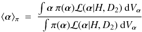 (15)where π(α) is the informative prior. Considerations of accuracy when values of χ2 are computed on a grid suggest we take to be the value at
 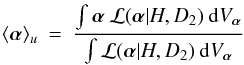 (16)the posterior mean for a uniform prior.
With and  thus defined, the Bayesian F is
  (17)and its value is to be compared with the chosen threshold Fν1,ν2,β when testing the consistency of X1 and X2. Since ⟨ α ⟩ u is independent of π(α), the statistic ℱ measures the effect of π(α) in displacing ⟨ α ⟩ π from ⟨ α ⟩ u.
In this Bayesian version of the F-test, the null hypothesis states that the posterior mean ⟨ α ⟩ π = αtrue. This will be approximately true when a flawless Bayesian model ℳ is applied to a flawless data set D. However, if the chosen threshold on ℱ is exceeded, then one or more of π,H and D is suspect as discussed in Sect. 3.1. If the threshold is not exceeded, then Bayesian inferences drawn from the posterior distribution p(α | H,D2) are supported.
6.3. Test of p-values from ℱ
If Eq. (17) gives ℱ = ℱ∗, the corresponding p-value is  (18)where ν1 = j and ν2 = n − i. The accuracy of these p-values can be tested with the 1D toy model of Sect. 5.1 as follows:
(i): Independent data sets D1,D2 are created corresponding to X1,X2.
(ii): With π from X1, the quantities  and ℱ∗ are calculated for X2 with Eqs. (15)–(17).
(iii): M independent data sets  are now created with
  .
.
(iv): For each  , the new value of
  is calculated for the derived at step (ii).
(v): For each , the new value of χ2( ⟨ α ⟩ u) is calculated with ⟨ α ⟩ u from Eq. (16).
(vi): With these new χ2 values, the statistic ℱm is obtained from Eq. (17).
The resulting M values of ℱm give us an empirical estimate of p∗, namely f∗, the fraction of the ℱm that exceed ℱ∗. In one example of this test, a data pair D1,D2 gives and ℱ∗ = 1.0021. With ν1 = 1 and ν2 = 99, Eq. (18) then gives p∗ = 0.3192. This is checked by creating M = 105 data sets with the assumption that μtrue = 0.089. The resulting empirical estimate is f∗ = 0.3189, in close agreement with p∗.
From 100 independent pairs D1,D2, the mean value of | p∗ − f∗ | is 0.001. This simulation confirms the accuracy of p-values derived from Eq. (18) and therefore of decision thresholds Fν1,ν2,β.
6.4. Bias test
To investigate this Bayesian F-test’s ability to detect inconsistecy between X1 and X2, the bias test of Sect. 5.2 is repeated, again with n1 = n2 = 100. The vector α in Sect. 6.1 now becomes the scalar μ, and i = 1.
In Fig. 3, the values of ℱ from Eq. (17) with j = i = 1 are plotted against the bias parameter b/σ. Also plotted are critical values derived from the distribution Fν1,ν2 with ν1 = 1 and ν2 = 99. In contrast to Fig. 2 for the ⟨ χ2 ⟩ π statistic, inconsistency between X1 and X2 is now detected down to b/σ ≈ 0.5.
In this test of inconsistency, the flaw in X1 is the bias b. Now, if it were known for certain that this was the flaw, then a Bayesian analysis with H1 changed from u = μ to u = μ + b – i.e., with an extra parameter – is staightforward. The result is the posterior density for b, allowing for correction. In contrast, the detection of a flaw with ⟨ χ2 ⟩ π or ℱ is cause-independent. Although Figs. 2 and 3 have b/σ as the abscissa, for real experiments this quantity is not known and conclusions are drawn just from the ordinate.
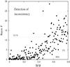 |
Fig. 3 Detection of inconsistency between X1 and X2. Values of ℱ are plotted against the bias parameter b/σ. The dashed lines are the 0.1, 5 and 50% levels. Note that the horizontal scale differs from Fig. 2. |
7. Tension between experiments
In the above, the goodness-of-fit of ℳ to D is investigated taking into account the possibility that a poor fit might be due the prior derived from a previous experiment. A related goodness-of-fit issue commonly arises in modern astrophysics, particularly cosmology, namely whether estimates of non-identical but partially overlapping parameter vectors from different experiments are mutually consistent. The term commonly used in this regard is tension, with investigators often reporting their subjective assessments – e.g., there is marginal tension between X1 and X2 – based on the two credibility domains (often multi-dimensional) for the parameters in common.
In a recent paper, Seehars et al. (2015) review the attempts in the cosmological literature to quantify the concept of tension, with emphasis on CMB experiments. Below, we develop a rather different approach based on the ℱ statistic defined in Sect. 6.2.
Since detecting and resolving conflicts between experiments is essential for scientific progress, it is desirable to quantify the term tension and to optimize its detection. The conjecture here is that this optimum is achieved when inferences from X1 are imposed on the analysis of X2.
7.1. Identical parameter vectors
A special case of assessing tension between experiments is that where the parameter vectors are identical. But this is just the problem investigated in Sects. 5 and 6.
When X1 (with bias) and X2 (without bias) are separately analysed, the limited overlap of the two credibility intervals for μ provides a qualitative indication of tension. However, if X2 is analysed with a prior derived from X1, then the statistic ⟨ χ2 ⟩ π – see Fig. 2 – or, more powerfully, the statistic ℱ – see Fig. 3 – provide a quantitative measure to inform statements about the degree of tension.
7.2. Non-identical parameter vectors-I
We now suppose that D1,D2 are data sets from different experiments X1,X2 designed to test the hypotheses H1,H2. However, though different, these hypotheses have parameters in common. Specifically, the parameter vectors of H1 and H2 are ξ = (α,β) and η = (β,γ), respectively, and k,l,m are the numbers of elements in α,β,γ, respectively.
If X1 and X2 are analysed independently, we may well find that ℳ1 and ℳ2 provide satisfactory fits to D1 and D2 and yet still be obliged to report tension between the experiments because of a perceived inadequate overlap of the two l-dimensional credibility domains for β.
A quantitative measure of tension between X1 and X2 can be derived via the priors, as follows: the analysis of X1 gives p(ξ | H1,D1), the posterior distribution of ξ, from which we may derive the posterior distribution of β by integrating over α. Thus  (19)Now, for a Bayesian analysis of X2, we must specify π(η) throughout η-space, not just β-space. But
  (20)Accordingly, what we infer from X1 can be imposed on the analysis of X2 by writing
  (21)The conditional prior π(γ | β) must now be specified. This can be taken to be uniform unless we have prior knowledge from other sources – i.e., not from D2.
With π(η) specified, the analysis of X2 gives the posterior density p(η | H2,D2). As in Sect. 6.2, we now regard this as a fuzzy constraint on η from which we compute the sharp constraint ⟨ η ⟩ π given by Eq. (15). Now, in general, ⟨ η ⟩ π will be displaced from ⟨ η ⟩ u given by Eq. (16). The question then is: Is the increment in χ2(η | H2,D2) between ⟨ η ⟩ π and ⟨ η ⟩ u so large that we must acknowledge tension between X1 and X2?
Following Sect. 6, we answer this question by computing ℱ from Eq. (17) with i = j = l + m, the total number parameters in η. The result is then compared to selected critical values from the Fν1,ν2 distribution, where ν1 = l + m and ν2 = n2 − l − m. With standard assumptions, ℱ obeys this distribution if ⟨ η ⟩ π = ηtrue – i.e., if ⟨ β ⟩ π = βtrue and ⟨ γ ⟩ π = γtrue – see Sect. 6.3.
7.3. A toy model
A simple example with one parameter (μ) for X1 and two (μ,κ) for X2 is as follows: H1 states that u = μ and H2 states that v = μ + κx. The data set D1 comprises n1 measurements ui = μ + σzi + b, where b is the bias. The data set D2 comprises n2 measurements vj = μ + κxj + σzj, where the xj are uniform in (− 1, + 1). The parameters are μ = 0,κ = 1,σ = 1 and n1 = n2 = 100. In the notation of Sect. 7.2, the vectors β,γ contract to the scalars μ,κ, whence l = m = 1, and α does not appear, whence k = 0.
7.4. Bias test
In the above, H1 are H2 are different hypotheses but have the parameter μ in common. If b = 0, the analyses of X1 are X2 should give similar credibility intervals for μ and therefore no tension. But with sufficiently large b, tension should arise.
This is investigated following Sect. 7.2. Applying ℳ1 to D1, we derive p(μ | H1,D1). Then, taking the conditional prior π(κ | μ) to be constant, we obtain  (22)as the prior for the analysis of X2. This gives us the posterior distribution p(μ,κ | H2,D2), which is a fuzzy constraint in (μ,κ)-space. Replacing this by the sharp constraint (⟨ μ ⟩ , ⟨ κ ⟩), the constrained χ2 is
  (23)Substitution in Eq. (17) with j = i = 2, then gives ℱ as a measure of the tension between X1 and X2. Under standard assumptions, ℱ is distributed as Fν1,ν2 with ν1 = 2,ν2 = n2 − 2 if (⟨ μ ⟩ , ⟨ κ ⟩ ) = (μ,κ)true.
In Fig. 4, the values of ℱ are plotted against b/σ together with critical values for Fν1,ν2 with ν1 = 2,ν2 = 98. This plot shows that tension is detected for b/σ ≳ 0.6. This is slightly inferior to Fig. 3 as is to be expected because of the more complicated X2.
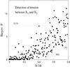 |
Fig. 4 Detection of tension between different experiments. Values of ℱ are plotted against the bias parameter b/σ. The dashed lines are the 0.1,5 and 50% levels. |
The importance of Fig. 4 is in showing that the ℱ statistic has the desired characteristic of reliably informing the investigator of tension between different experiments with partially overlapping parameter vectors. When the inconsistency is slight (b/σ ≲ 0.2), this statistic does not sound a false alarm. When the inconsistency is substantial (b/σ ≳ 0.6), the statistic does not fail to sound the alarm.
7.5. Non-identical parameter vectors-II
If ℱ calculated as in Sect. 7.2 indicates tension, the possible flaws include the conditional prior π(γ | β). Thus, tension could be indicated even if the prior π(β) inferred from X1 is accurate and consistent with D2.
Accordingly, we might prefer to focus just on β – i.e., on the parameters in common. If so, we compute  (24)and then find the minimum of χ2(η | H2,D2) when β = ⟨ β ⟩ π. Thus, the contrained χ2 is now
  (25)The F test also applies in this case – see Sect. 6.1. Thus this value is substituted in Eq. (17), where we now take j = l, the number of parameters in β. The resulting ℱ is then compared to critical values derived from Fν1,ν2 with ν1 = l,ν2 = n2 − l − m. With the standard assumptions, ℱ obeys this distribution if ⟨ β ⟩ π = βtrue.
For the simple model of Sect. 7.3, the resulting plot of ℱ against b/σ is closely similar to Fig. 4 and so is omitted. Nevertheless, the option of constraining a subset of the parameters is likely to be a powerful diagnostic tool for complex, multi-dimensional problems, identifying the parameters contributing most to the tension revealed when the entire vector is constrained (cf. Seehars et al. 2015).
8. Discussion and conclusion
A legitimate question to ask about the statistical analysis of data acquired in a scientific experiment is: How well or how badly does the model fit the data? Asking this question is, after all, just the last step in applying the scientific method. In a frequentist analysis, where the estimated parameter vector α0 is typically the minimum-χ2 point, this question is answered by reporting the goodness-of-fit statisic  or, equivalently, the corresponding p-value. If a poor fit is thereby indicated, the investigator and the community are aware that not only is the model called into question but so also is the estimate α0 and its confidence domain.
If the same data is subject to a Bayesian analysis, the same question must surely be asked: the Bayesian approach does not exempt the investigator from the obligation to report on the success or otherwise of the adopted model. In this case, if the fit is poor, the Bayesian model is called into question and so also are inferences drawn from the posterior distribution p(α | H,D).
As noted in Sect. 1, the difficulty in testing Bayesian models is that there are no good fully Bayesian methods for assessing goodness-of-fit. Accordingly, in this paper, a frequentist approach is advocated. Specifically, ⟨ χ2 ⟩ π is proposed in Sect. 3 as a suitable goodness-of-fit statisic for Bayesian models. Under the null hypothesis that ℳ and D are flawless and with the standard assumptions of linearity and normally-distributed errors, then, as argued in Sect. 4.1 and illustrated in Fig. 1, ⟨ χ2 ⟩ π − k is approximately distributed as  , and so p-values can be computed. A p-value thus derived from ⟨ χ2 ⟩ π quantifies the average goodness-of-fit provided by the posterior distribution. In contrast, in a frequentist minimum-χ2 analysis, the p-value quantifies the goodness-of-fit provided by the point estimate α0.
In the above, it is regarded as self-evident that astronomers want to adhere to the scientific method by always reporting the goodness-of-fit achieved in Bayesian analyses of observational data. However, Gelman & Shalizi (2013), in an essay on the philosophy and practice of Bayesian statistics, note that investigators who identify Bayesian inference with inductive inference regularly fit and compare models without checking them. They deplore this practice. Instead, these authors advocate the hypothetico-deductive approach in which model checking is crucial. As in this paper, they discuss non-Bayesian checking of Bayesian models – specifically, the derivation of p-values from posterior predictive distributions. Moreover, they also stress that the prior distribution is a testable part of a Bayesian model.
In the astronomical literature, the use of frequentist tests to validate Bayesian models is not unique to this paper. Recently, Harrison et al. (2015) have presented an ingenious procedure for validating multidimensional posterior distributions with the frequentist Kolmogorov-Smirnov (KS) test for one-dimensional data. Their aim, as here, is to test the entire Bayesian inference procedure.
Frequentist testing also arises in recent applications of the Kullback-Leibler divergence to quantify tension between cosmological probes (e.g. Seehars et al. 2015). For linear models, and with the assumption of Gaussian priors and likelihoods, a term in the relative entropy is a statistic that measures tension. With these assumptions, the statistic follows a generalized χ2 distribution, thus allowing a p-value to be computed.
Seehars et al. (2015) also investigate various purely Bayesian measures of tension. They conclude that interpreting these measures on a fixed, problem-independent scale – e.g., the Jeffrey’s scale – can be misleading – see also Nesseris & García-Bellido (2013).
Acknowledgments
I thank D. J. Mortlock for comments on an early draft of this paper, and A. H. Jaffe, M.P.Hobson and the referee for useful references.
References
- Bridges, M., Feroz, F., Hobson, M. P., & Lasenby, A. N. 2009, MNRAS, 400, 1075 [NASA ADS] [CrossRef] [Google Scholar]
- Feldman, G. J., & Cousins, R. D. 1998, Phys. Rev. D, 57, 3873 [Google Scholar]
- Gelman, A., & Shalizi 2013, British J. Math. Stat. Psychol., 66, 8 [CrossRef] [Google Scholar]
- Hamilton, W. C. 1964, Statistics in Physical Science (New York: Ronald Press) [Google Scholar]
- Harrison, D., Sutton, D., Carvalho, P., & Hobson, M. 2015, MNRAS, 451, 2610 [NASA ADS] [CrossRef] [Google Scholar]
- Lucy, L. B. 2014, A&A, 571, A86 (L14) [NASA ADS] [CrossRef] [EDP Sciences] [Google Scholar]
- Nesseris, S., & García-Bellido, J. 2013, J. Cosmol. Astropart. Phys., 08, 036 [NASA ADS] [CrossRef] [Google Scholar]
- Press, W. H., Teukolsky, S. A., Vetterling, W. T., & Flannery, B. P. 2007 Numerical Recipes (Cambridge: Cambridge University Press) [Google Scholar]
- Seehars, S., Grandis, S., Amara, A., & Refregier, A. 2015, arXiv e-prints [arXiv:1510.08483] [Google Scholar]
- Sellke, T., Bayarri, M. J., & Berger, J. 2001, The American Statistician, 55, 62 [CrossRef] [Google Scholar]
- Sivia, D. S., & Skilling, J. 2006, Data Analysis: A Bayesian Tutorial, 2nd Edn. (Oxford: Oxford University Press) [Google Scholar]
Appendix A: Evaluation of ⟨ χ2 ⟩ u
If α0 denotes the minimum-χ2 solution, then  (A.1)where a is the displacement from α0. Then, on the assumption of linearity,
  (A.2)where the Aij are the constant elements of the k × k curvature matrix (Press et al. 2007, p. 680), where k is the number of parameters. It follows that surfaces of constant χ2 are k-dimensional self-similar ellipsoids centered on α0.
Now, given the second assumption of normally-distributed measurement errors, the likelihood  (A.3)Thus, in the case of a uniform prior, the posterior mean of χ2 is
  (A.4)
(A.4)
Because surfaces of constant Δχ2 are self-similar, the k-dimensional integrals in Eq. (A.4) reduce to 1D integrals.
Suppose  on the surface of the ellipsoid with volume V∗. If lengths are increased by the factor λ, then the new ellipsoid has
  (A.5)With these scaling relations, the integrals in Eq. (A.4) can be transformed into integrals over λ. The result is
  (A.6)where
  . The integrals have now been transformed to a known definite integral,
  (A.7)where x = (z + 1) / 2. Aplying this formula, we obtain
  (A.8)an exact result under the stated assumptions.
All Figures
|
Fig. 1 Empirical PDF of ⟨ χ2 ⟩ π derived from the analysis of 106 data pairs D1,D2 as described in Sect. 5.1. The dashed curve is the theoretical PDF for ⟨ χ2 ⟩ u. |
| In the text | |
|
Fig. 2 Detection of bias in X1 with the ⟨ χ2 ⟩ π statistic when X2 is analysed with prior derived from X1. Values of ⟨ χ2 ⟩ π (filled circles) and ⟨ χ2 ⟩ u (open circles) are plotted against the bias parameter b/σ. The dashed lines are the 5 and 95% levels. |
| In the text | |
|
Fig. 3 Detection of inconsistency between X1 and X2. Values of ℱ are plotted against the bias parameter b/σ. The dashed lines are the 0.1, 5 and 50% levels. Note that the horizontal scale differs from Fig. 2. |
| In the text | |
|
Fig. 4 Detection of tension between different experiments. Values of ℱ are plotted against the bias parameter b/σ. The dashed lines are the 0.1,5 and 50% levels. |
| In the text | |
Current usage metrics show cumulative count of Article Views (full-text article views including HTML views, PDF and ePub downloads, according to the available data) and Abstracts Views on Vision4Press platform.
Data correspond to usage on the plateform after 2015. The current usage metrics is available 48-96 hours after online publication and is updated daily on week days.
Initial download of the metrics may take a while.