| Issue |
A&A
Volume 588, April 2016
|
|
|---|---|---|
| Article Number | A2 | |
| Number of page(s) | 15 | |
| Section | Planets and planetary systems | |
| DOI | https://doi.org/10.1051/0004-6361/201527675 | |
| Published online | 09 March 2016 | |
The long-wavelength thermal emission of the Pluto-Charon system from Herschel observations. Evidence for emissivity effects⋆
1 LESIA, Observatoire de Paris, PSL Research University, CNRS, Sorbonne Universités, UPMC Univ. Paris 06, Univ. Paris Diderot, Sorbonne Paris Cité, 5 place Jules Janssen, 92195 Meudon, France
e-mail: This email address is being protected from spambots. You need JavaScript enabled to view it.
2 Instituto de Astrofísica de Andalucía-CSIC, Glorieta de la Astronomía s/n, 18008 Granada, Spain
3 European Space Astronomy Centre (ESAC), PO Box 78, 28691 Villanueva de la Cañada, Madrid, Spain
4 Space Telescope Science Institute, 3700 San Martin Drive, Baltimore, MD 21218, USA
5 Max-Planck-Institut für Sonnensystemforschung, Justus-von-Liebig-Weg 3, 37077 Göttingen, Germany
6 Max-Planck-Institut für Extraterrestrische Physik, Giessenbachstraße, 85748 Garching, Germany
7 Konkoly Observatory of the Hungarian Academy of Sciences, Konkoly Thege Miklós út 15-17, 1121 Budapest, Hungary
8 Department of Astronomy, University of Maryland, College Park, MD 20742, USA
9 GEPI, Observatoire de Paris, PSL Research University, CNRS, Univ. Paris Diderot, Sorbonne Paris Cité, 5 place Jules Janssen, 92195 Meudon, France
Received: 2 November 2015
Accepted: 21 December 2015
Abstract
Thermal observations of the Pluto-Charon system acquired by the Herschel Space Observatory in February 2012 are presented. They consist of photometric measurements with the PACS and SPIRE instruments (nine visits to the Pluto system each), covering six wavelengths from 70 to 500 μm altogether. The thermal light curve of Pluto-Charon is observed in all filters, albeit more marginally at 160 and especially 500 μm. Putting these data into the context of older ISO, Spitzer and ground-based observations indicates that the brightness temperature (TB) of the system (rescaled to a common heliocentric distance) drastically decreases with increasing wavelength, from ~53 K at 20 μm to ~35 K at 500 μm, and perhaps ever less at longer wavelengths. Considering a variety of diurnal and/or seasonal thermophysical models, we show that TB values of 35 K are lower than any expected temperature for the dayside surface or subsurface of Pluto and Charon, implying a low surface emissivity. Based on multiterrain modeling, we infer a spectral emissivity that decreases steadily from 1 at 20−25 μm to ~0.7 at 500 μm. This kind of behavior is usually not observed in asteroids (when proper allowance is made for subsurface sounding), but is found in several icy surfaces of the solar system. We tentatively identify that a combination of a strong dielectric constant and a considerable surface material transparency (typical penetration depth ~1 cm) is responsible for the effect. Our results have implications for the interpretation of the temperature measurements by REX/New Horizons at 4.2 cm wavelength.
Key words: planets and satellites: surfaces / Kuiper belt objects: individual: Pluto / methods: observational / techniques: photometric / Kuiper belt objects: individual: Charon
Herschel is an ESA space observatory with science instruments provided by European-led Principal Investigator consortia and with important participation from NASA.
© ESO, 2016
1. Introduction
The New Horizons flyby of the Pluto system on July 14, 2015 revealed Pluto and Charon as planetary worlds (Stern et al. 2015). Pluto appears to display an unexpected variety of terrain morphologies, suggesting a complex history of surface activity. These include icy plains with evidence for glacier-like flows of ice and polygonal ice patterns, mountain ridges several kilometers high, and dark, cratered, ancient terrains, where irradiation of surface ices (N2, CH4, CO) and/or atmospheric production of organic tholins falling to the surface may be responsible for the dark red color. While the identification of the processes shaping this rich geology is just beginning, it already seems clear that Pluto’s surface appearance is to a large extent sculpted by interactions between its mobile volatile ices, evolving N2-dominated atmosphere, and surface bedrock. Mars-like seasonal cycles must be at work, in which volatile N2 (and the secondary species CH4 and CO) are shared between atmospheric and surface ice reservoirs through sublimation/condensation exchanges and volatile migration. These processes are related to the temperature distribution across Pluto’s surface, which reflects the balance between insolation, thermal radiation, thermal conduction, and latent heat exchanges, and depends on important parameters such as albedo, emissivity, and thermal inertia (see, e.g., Hansen & Paige 1996; Young 2012). At Charon, where no atmosphere has yet been detected, such resurfacing processes are less obvious, although the distinctly red color of Charon’s north polar region may be related to seasonal cold trapping of volatiles in that region, followed by energetic radiation (Stern et al. 2015).
Temperature measurements on an icy surface are possible from the temperature-dependent position and shape of near-IR absorption bands (e.g., Quirico & Schmitt 1997; Tryka et al. 1994, 1995; Grundy et al. 1999, 2002). This diagnostic is to be used by New Horizons/Ralph (Reuters et al. 2008), for example, for the N2(2−0) ice band at 2.15 μm. The only other method for determining surface temperatures is thermal radiometry. Thermal measurements (in general spatially unresolved) of the Pluto system at a variety of wavelengths (from ~20 to 1400 μm) have been acquired using IRAS, ISO, and Spitzer, and a number of ground-based mm/submm facilities. In particular, the ISO and Spitzer measurements clearly detected the Pluto+Charon thermal light curve that is associated with the albedo contrasts on Pluto and the diurnal variability of insolation. These measurements have provided the first determination of the thermal inertia of Pluto and Charon, and some constraints on their emissivity behavior over 20−160 μm (Lellouch et al. 2000a, 2011).
The operation of Herschel (Pilbratt et al. 2010) in 2009−2013 offered an opportunity to extend the study toward longer wavelengths (70−500 μm), bridging the gap with the sub-mm/mm measurements. Combined with previous Spitzer data, these measurements permit us to refine our estimates of Pluto’s and Charon’s thermal inertia, and determine the long-wavelength behavior of the system’s emission. Following an initial assessment of the data (Lellouch et al. 2013a), we present a detailed report of these observations and their modeling. The Herschel 70-μm data that are described below have already been used to derive limits on the amount of dust in the Pluto–Charon system (Marton et al. 2015).
Summary of observations.
2. Herschel observations
We obtained thermal photometry of the Pluto system with the two imaging photometers of Herschel, Photoconductor Array Camera and Spectrometer (PACS; Poglitsch et al. 2010) and Spectral and Photometric Imaging Receiver (SPIRE; Griffin et al. 2010), covering altogether six wavelengths. The SPIRE instrument observes a 4′ × 8′ field simultaneously in three bolometer arrays at 250 μm, 350 μm, and 500 μm, with respective pixel sizes of 6′′, 10′′, and 13′′. PACS can operate in three filters, centered at 70 μm (“blue”), 100 μm (“green”), and 160 μm (“red”). However, as it includes two detector arrays (64 × 32 pixels of 3.2″ × 3.2″ for blue/green and 32 × 16 pixels of 6.4″ × 6.4″ for red, each of them covering a FOV of 3.5′ × 1.75′), only two filters out of three (70/160 μm or 100/160 μm) are observed in parallel.
For both instruments, the beam size (17″−35″ FWHM for SPIRE and 5″−11″ FWHM for PACS, depending on filter) encompassed the entire ~1′′-wide Pluto system, thus including thermal emission from Pluto and Charon (with a negligible contribution from the other four moons). All data were acquired over three weeks in late February to mid-March 2012, under the OT2_elellouc_2 program (“Pluto’s seasonal evolution and surface thermal properties”). We acquired nine observations of the Pluto system with each instrument. They were timed to sample equally-spaced subobserver longitudes, so as to provide a multiband thermal light curve. In practice, consecutive visits to Pluto were scheduled with a time separation of ~17 h, equivalent to ~40° longitude. The SPIRE observations occurred over Feb. 29−Mar. 6, 2012, while the PACS data were taken on Mar. 14−19, 2012. Pluto’s heliocentric distance at that time was rh = 32.19 AU, the subsolar latitude was β = 47.0°, and the phase angle was 1.6°.
We acquired the SPIRE observations in the small-map mode. The telescope was scanned across the sky at 30′′/s, in two nearly orthogonal (84.8° angle) scan paths, uniformly covering an area of 5′ × 5′. Each SPIRE visit to Pluto amounted to 1421 s, corresponding to ten repetitions of the scanning pattern.
We used the mini scan map mode for PACS, which has been demonstrated to be more sensitive than the point-source (chop-nod) mode (Müller et al. 2010)1. For each filter combination (70/160 μm or 100/160 μm), we acquired data consecutively in two scanning directions (termed “A” and “B”), with 70° and 110° angles with respect to the detector array and individual integration times of 286 s per scan, i.e., 1144 s (4 repetitions) per PACS visit. Observational details are given in Table 1, where the A-B scanning sequences are indicated by consecutive Obs. ID numbers.
Far-infrared photometry can often be plagued by confusion noise, i.e., spatial variations in the sky emission at scales comparable to the point spread function (PSF). The confusion noise is typically ~5−7 mJy/beam in the SPIRE bands (Nguyen et al. 2010) and lower in the PACS bands, but Pluto’s 2012 position in star-crowded regions of Sagittarius not far from Galactic center made sky background levels a priori more severe. Estimates of confusion levels at proposal stage indicated that even though the March 2012 epoch was most favorable in this respect (and selected for that reason), it would be subject to confusion noise at the ~5 and ~20 mJy in the PACS 100 μm and 160 μm beams, respectively, i.e., a non-negligible fraction of the expected fluxes from Pluto (~400 and 300 mJy, respectively). However, the proper motion of Pluto offered the possibility to observe the target several times against different sky backgrounds, permitting us to subtract the sky contribution. The efficiency of this “follow-on” (a.k.a. second-visit) approach has been demonstrated by the detection of numerous TNOs at the mJy level by Spitzer and Herschel (e.g., Stansberry et al. 2008; Santos-Sanz et al. 2012). For the technique to work, the proper motion between two visits should be significantly larger than the PSF size, but remain small enough that at the second visit, the object still falls within the high-coverage area of the map from the first visit. In practice, these conditions are best met for proper motions of 30″−50″ for PACS observations and 72′′−150′′ for SPIRE. In our observing sequence, the proper motion of Pluto between two consecutive visits (~17 h separation) was of 55−35 arcsec, almost entirely in the RA direction (and decreasing with time as Pluto approached stationarity on April 10, 2012). Thus, for PACS observations, each visit to Pluto could be used as second epoch measurement for the preceding and/or following visit (17 h before or after). For SPIRE, we often used more distant visits (i.e., 34 or 51 h before or after a given observation) for the second epoch, as difference maps between two contiguous visits would result in the positive and negative Pluto images in the differential map to partially overlap at 500 μm.
3. Data reduction
PACS: Data reduction was initially performed within the Herschel interactive processing environment (HIPE; Ott 2010), version 12, using its default FM7 calibration scheme and an optimum script for “bright” sources. Each PACS visit to Pluto provides two images (A and B scans) at 70 μm and 100 μm, and four images at 160 μm. For the green (100 μm) and red (160 μm) data, each image of a given visit was analyzed in combination with the corresponding image of the previous (“before”) or successive (“after”) visit to Pluto. The exception to this was, of course, for the first (resp. last) visit to Pluto for which only the “after” (resp. “before”) image could be used. This permitted us to generate two background maps, which were then subtracted from the individual image, providing a cleaner map suited for photometry. Standard aperture photometry on the resulting difference image was performed with our own IRAF/DAOPHOT-based routines via a curve-of-growth approach to determine the optimum synthetic aperture and a Monte-Carlo method of 200 fictitious source implantations to estimate error bars (see Santos-Sanz et al. 2012 and Kiss et al. 2014 for details). The method thus provided in general (i.e., except for the first and last visit, for which two times fewer values were obtained) four (in the green) or eight (in the red) individual values of the flux (fi, error bar σi) per visit. The sky subtraction did not bring any noticeable improvement for blue (70-μm) data, which have the least background contamination. Therefore, we simply performed aperture photometry on the original A and B images, providing two sets of values per visit. The optimum aperture radii were found to be 5.5′′, 7.0′′, and 10.5′′ in the blue, green, and red bands, respectively, i.e., close to the PSF full width at half maximum at the corresponding wavelengths. For each filter and visit, the 2 to 8 (1 to 4 for first and last visit) individually-determined fluxes were (error-bar weighted) averaged. To be conservative, we took the final error on the average flux to be max (std(fi), 1/ ), where std(fi) is the standard deviation of the individual fluxes. Minor color corrections were finally applied, by dividing the averaged fluxes and their error bars by factors of 0.983 (70-μm), 0.982 (100-μm), and 1.000 (160-μm), appropriate (to within ±0.01) for respective color temperatures of 47 K, 45 K, and 43 K. The final flux values are gathered in Table 1. Additional systematic calibration uncertainties (5% of the measured flux), which do not affect the light curves, are not included in Table 1.
SPIRE: SPIRE data were first processed using HIPE, version 10, including de-striping routines that minimize background differences between data acquired at different epochs and that properly correct the signal timeline. Then, maps were produced using the standard naive map-making, projecting the data of each band on the same World Coordinate System (WCS) and applying cross-correlation routines between two epochs to correct for astrometry offsets. Finally, for each Pluto visit, several difference maps were computed at each band by subtracting, from the map under consideration, maps taken at other epochs, separated by ~±17, ±34 and/or ±51 h (also depending on the considered filter). Photometry on these difference maps was then performed with a two-dimensional circular Gaussian aperture with a fixed filter-dependent FWHM (PSF fitting), following the method described in Fornasier et al. (2013). The derived flux was then corrected by the instrument pixellization factors, i.e., dividing by 0.951, 0.931, and 0.902 for 250, 350, and 500 μm, respectively. Finally, color corrections were estimated by convolving a blackbody emission at 35−40 K, the approximate system brightness temperature at the SPIRE wavelengths, with the instrument spectral response profiles. These multiplicative color correction factors were found to be 0.974, 0.976, and 0.957 at 250, 350, and 500 μm, and applied to the individual Pluto-Charon fluxes. The final system flux for each visit was then computed as the weighted mean of the individual fluxes based on the various differential maps (in a few cases after rejecting some outliers). Final fluxes with all corrections included are gathered in Table 1. Similar to PACS, the errors include the uncertainties provided by the Gaussian fitting algorithm, but do not account for absolute calibration uncertainties, which are estimated to be 7% of the measured flux. The final PACS and SPIRE fluxes were converted into system brightness temperatures (TB) by assuming a 1185 km radius for Pluto and 604 km for Charon. The Charon radius is based on stellar occultation (Sicardy et al. 2006). The adopted Pluto radius is close to the best guess value from Lellouch et al. (2015), 1184 km. These values match initial reports from New Horizons (606 ± 3 km and 1187 ± 4 km; Stern et al. 2015). Results would be insignificantly sensitive to further changes of the radii by a few kilometers. The adopted value for Pluto’s radius updates the value that was used in previous modeling of the ISO and Spitzer data (1170 km). The effect is negligible at 24 μm (a ~0.1 K decrease in the TB) but not entirely so at 500 μm (~0.5 K decrease).
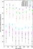 |
Fig. 1 Pluto-Charon thermal light curves in the six filters observed with PACS and SPIRE. |
4. Modeling
4.1. Qualitative analysis
Brightness temperatures of the Pluto-Charon system over 70−500 μm as a function of rotational phase are shown in Fig. 1. Immediately apparent in the figure is that: (i) the mean brightness temperature (TB) of the system decreases steadily with increasing wavelength from ~46.5 K at 70 μm to ~35 K at 500 μm; and (ii) the thermal light curve is detected at all wavelengths, albeit somewhat marginally at 160 μm and especially 500 μm, given the higher error bars of these data. At 70 and 160 μm, the data are of much higher quality than was possible from Spitzer (see Fig. 2 from Lellouch et al. 2011, hereafter Paper I). All data are consistent with maximum flux near an east longitude L = 60−80 and minimum flux near L = 200−220. More quantitatitively, sinusoidal fits to the data yield flux maxima at L = 57 ± 5, 50 ± 8, 42 ± 22, 57 ± 10, 76 ± 17, and 70 ± 60 for 70, 100, 160, 250, 350, and 500-μm data. Thus, within measurements uncertainties, all light curves appear in phase (in particular, there is excellent phase agreement between the 70 μm, 100 μm and 250 μm data). Out-of-phase light curves at the longest wavelengths had been envisaged in Paper I.
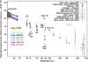 |
Fig. 2 Brightness temperature (TB) of the Pluto system. Most thermal observations from ISO, Spitzer, Herschel, and ground-based telescopes are gathered. As data were acquired at different epochs spanning ~25 yr, the TB are rescaled by 1/ |
In Fig. 2, the Herschel measured brightness temperatures are plotted as a function of wavelength and put into the broader context of most previous thermal measurements of the Pluto-Charon system. These measurements include (i) ISOPHOT 60, 100, 150, and 200 μm photometry, taken mostly in Feb.-March 1997 (five to eight visits to Pluto; Lellouch et al. 2000a); (ii) Spitzer/MIPS 23.68, 71.42, and 156 μm photometry and Spitzer/IRS low-resolution spectroscopy over 20−37 μm recorded in August-September 2004 (eight visits to Pluto each; Paper I); (iii) additional Spitzer/MIPS data at 23.68 and 71.42 μm taken in April 2007 (12 visits; see Fig. 13 of Paper I), and unpublished 156 μm data from October 2008 (12 visits); and (iv) a number of ground-based measurements at mm/sub-mm wavelengths from IRAM, JCMT, and SMA (Altenhoff et al. 1988; Stern et al. 1993; Jewitt 1994; Lellouch et al. 2000b; Gurwell et al. 2011). We emphasize that the SMA data separate Pluto from Charon, and we report the Pluto-only TB from 2005 and 2010. In Fig. 2, Spitzer/MIPS and IRS data from 2004 at eight longitudes are plotted individually. We reinterpolate, to the same eight longitudes, the Herschel (70, 100, 160, 250, 350, and 500 μm), Spitzer 71.42 μm from 2007, and ISO 60 and 100 μm data, all of which clearly show light curves. For data in which we did not discern (or attempt to detect) a light curve, i.e., ISO 150 and 250 μm, Spitzer 156 μm from October 2008, and all of the ground-based data, we simply plotted the mean TB averaged over the available measurements. All of the ISO, Spitzer, and Herschel TB in Fig. 2 make consistent use of the above Pluto and Charon radii. In contrast, mm/sub-mm TB simply use published values, because of the difficulty in tracking down the originally used radii. All these thermal measurements span 25 years (1986−2012), a period over which Pluto’s heliocentric distance (rh) and subsolar latitude (β) varied from 29.7 AU to 32.2 AU and from −4° to +47°, respectively. While the effect of a change in the subsolar latitude cannot be accounted for without a detailed model, the effect of varying rh is handled by rescaling the measured TB by 1/ to the epoch of the Spitzer 2004 data (rh = 30.847 AU).
Figure 2 illustrates a number of important features. (i) The difficult-to-explain Pluto “fading” witnessed by Spitzer, i.e., the decrease by ~2 K of the 71 μm TB (and by ~0.5 K at 24 μm) over 2004−2007 (Paper I) is not confirmed in the Herschel data, which indicates 70-μm TB in good agreement with the Spitzer 2004 data. (ii) The 150−160 μm TB show large dispersion. While the original ISO-150 μm data (Lellouch et al. 2000a) indicated anomalously high fluxes (T ≥ 50 K in average), the Spitzer/MIPS 156 μm data from April 2004 instead pointed to TB< 40 K. The additional Spitzer/MIPS 156 μm unpublished data from October 2008 (12 visits) indicate a mean (rescaled) value of 45.3 K with a formal error of 1 K, but a 5.2 K dispersion over the 12 visits, which is a more likely representation of actual uncertainty. This mean value is generally in line, albeit somewhat on the higher side, with the 160 μm TB indicated by Herschel. (iii) The ensemble of data clearly outlines the decrease of the system brightness temperature with wavelength over the entire thermal range (λ> 20μm). Although data in the sub-mm/mm range show large dispersion, the most accurate of them (i.e., the SMA data from 2010 Gurwell et al. 2011 and the IRAM Feb.-Mar. 2000 data from Lellouch et al. 2000b) point to a ~32 K brightness temperature at 1100−1300 μm, i.e., a consistent “extrapolation” of the trend indicated by the Herschel data into the mm range. Thus it appears that the Pluto-Charon TB decreases by more than 30% of its value from 20 μm (~53 K) to 500 μm (~35 K) and beyond.
4.2. Emissivity
Qualitatively, a decreasing TB with increasing wavelength can be produced in several ways: (i) a spatially constant surface temperature T and a low (but spectrally constant) surface emissivity; (ii) the mixing of different surface temperatures. Such a mixing can occur both on regional scales (e.g., different Pluto and Charon regions have different temperatures because of different albedos or because they see different instantaneous insolations) and on small scales (slopes at any scales, i.e., surface roughness, cause adjacent surface facets to see large variations of temperatures due to shadows and/or re-radiation); and (iii) a decrease of the spectral emissivity with wavelength. Scenario (i) is technically possible, but fitting the Herschel-measured brightness temperatures over 70−500 μm would require a constant T ~ 52.5 K and an improbably low (~0.57) spectrally constant surface emissivity. Rather, given the observed albedo variegation on Pluto and Charon, scenario (ii) must occur, at least on geographic scales. Based on multiterrain modeling of the Spitzer data, however, Paper I found that a decrease of the spectral emissivity with wavelength, i.e. scenario (iii), of some of the Pluto areas (the CH4 ice regions) was also required.
Spectral “emissivity” is often loosely defined in the literature, and sometimes treated as a fudge factor in models. In essence, it represents the ratio of the observed fluxes to model fluxes, but how much physics is put into the models leads to different estimates of the “emissivity”. In early works, surface temperatures were described in simplistic end-member cases, such as the “nonrotating” or the “rapid rotator” cases. The advent of more elaborate models, such as the asteroid STM (Lebofsky et al. 1986) and NEATM (Harris 1998), and of physically-based, thermophysical models (TPM; e.g., Spencer et al. 1989; Lagerros 1996; Müller & Lagerros 1998), provided a more realistic description of the surface temperature distribution across airless bodies, and thereby a definition of spectral emissivity in reference to fluxes emitted from the surface. However, a further complication is that, particularly at long wavelengths, the surface materials’ partial transparency may cause the emitted radiation not to originate at the surface itself, but from some characteristic depth that depends on the material absorption coefficient. Therefore, the emitted flux does not just depend on the surface temperature, but on the thermal profiles T(z) within the subsurface. Consideration of this aspect leads to another definition of the emissivity, as the ratio of the observed to the modeled fluxes. The modeled flux, Φν, at some frequency ν, is expressed locally as, e.g., (Keihm et al. 2013)  (1)and spatially integrated over the object. Here Bν is the Planck function, Le is the electrical skin depth (inverse of the absorption coefficient), and μ is the viewing geometry dependent angle between the outgoing radiation and the surface normal.
Many asteroid studies (e.g., Redman et al. 1998; Müller & Lagerros 1998), making use of surface temperature for reference, reported evidence for very low spectral emissivities (0.6−0.7) in the mm/sub-mm ranges, which were attributed to grain size dependent subsurface scattering processes. However, the recent comprehensive study by Keihm et al. (2013) demonstrated that when allowance is made for subsurface sounding (and for the enhancement of the infrared fluxes by surface roughness), the observed mm/sub-mm fluxes are generally consistent with spectral emissivities close to 1 (e.g., 0.95). This suggests that no scattering losses occur, except for specular reflection at the surface, which can be characterized by a Fresnel coefficient with moderate (~2.3) dielectric constant, characteristic of low-density material. As discussed below, however, there are other planetary surfaces where thermal scattering effects are demonstrated to occur.
In our previous works (Lellouch et al. 2000a, 2011), the emissivity required to match the observed ISO or Spitzer fluxes was defined in reference to a thermophysical model that only considered the surface temperatures. A complication was related to the multiplicity of surface terrains. Three units (N2 ice, CH4 ice, tholin/H2O ice) were considered for Pluto and one for Charon, and the approach was to (i) fix the spectral and bolometric emissivity of all units except CH4 and (ii) adjust them for the CH4 unit, using for initial guidance expectations based on spectral properties of ices (Stansberry et al. 1996a). Results (Paper I) suggested a large decrease of the spectral emissivity of CH4 ice, from ~1 at 24 μm to ~0.4 at 200 μm. However, possible subsurface sounding effects were not considered, except in Lellouch et al. (2000b), where the nondetection of the 1.2 mm light curve was interpreted in terms of the mm-emissivity of the tholin/H2O ice unit. Furthermore, all of our previous thermophysical models were “diurnal-only”, i.e., they assumed equilibrium of the diurnally averaged temperatures with the instantaneous seasonal insolation. Thermal inertia effects on seasonal timescales are thought to be important in controlling the surface-atmosphere exchanges (Young 2012, 2013; Olkin et al. 2015; Hansen et al. 2015) and the atmospheric pressure. They may be important to include for our purposes because they are likely to impact the near-surface temperatures.
Along with the decreasing brightness temperatures with increasing wavelength, a striking result of the Herschel measurement is the low TB value (~35 K) at 500 μm. Below we demonstrate that such a TB is lower than any expected value for the dayside surface or subsurface of these bodies; thus, subsurface sounding toward the longest wavelengths is not the only cause of the decreasing TB, so that “true” emissivity effects (as defined per Eq. (1)) must occur.
4.3. Thermal modeling
One complication associated with modeling of long-wavelength thermal data is related to the unknown level probed by the emission within the surface, compared to the depth over which temperature changes occur (the thermal skin depth). Unlike in the thermal IR (e.g., 10−50 μm), where radiation is emitted from the surface itself (within a fraction of a mm), materials can be transparent enough in the sub-mm that thermal radiation might originate from layers ~10 to several thousand times the wavelength (i.e., 5 mm to 1 m or more at 500 μm). The thermal skin depth is related to the thermal inertia Γ through ds = 
 , where ρ is density, c is heat capacity, and P is the (diurnal or orbital) period. The parameter ds is therefore not completely defined by Γ since ρ and c may not be well known2. Still, using typical numbers for ρ (900 kg m-3) and c (400 J kg-1K -1), a thermal inertia Γ = 25 J m-2 s-0.5 K-1 (hereafter MKS) for Pluto leads to a diurnal skin depth of 3 cm, meaning that sub-mm radiation could either probe within or below the diurnal skin depth and conceivably could even encompass a substantial fraction of the seasonal skin depth (3.5 m for Γ = 25 MKS). A much larger thermal inertia (Γ = 1000−3000 MKS) could be more appropriate on seasonal timescales (Olkin et al. 2015), however; then the seasonal skin depth would extend several hundreds of meters deep.
Given these uncertainties, our initial approach is to consider a number of situations of relative electrical, diurnal, and seasonal skin depths. For that we first model horizontal and vertical temperatures of a “mean” Pluto using a standard spherical thermophysical model (Spencer et al. 1989)3. By “mean Pluto”, we mean that we use a Bond albedo of 0.46 derived from a mean geometric albedo pV = 0.58 and a plausible phase integral q = 0.8 (Lellouch et al. 2000a; Brucker et al. 2009). A bolometric emissivity of 1.0 is assumed and no surface roughness effects are included. As discussed below, the model is not relevant to the N2-ice covered areas whose heat budget is affected by sublimation/condensation terms.
4.3.1. Diurnal-only models
As a first step, we consider a “diurnal-only” model. In this case, the local insolation is calculated using “fixed” heliocentric distance and subsolar latitude relevant to early March 2012, which leads in particular to zero temperatures in the polar night southward of 43°S4. A thermal inertia of 25 MKS is assumed, following results from Paper I. Figure 3 shows the resulting (i) surface temperatures and (ii) “subdiurnal” temperatures, i.e., temperatures at depths much below the diurnal skin depth, in both cases as seen from the observer (neglecting the small 1.6° phase angle). Surface temperatures (relevant to dayside) peak near ~56 K at high northern latitudes and fall below 35 K at latitudes below 20° S only. Subdiurnal temperatures, which follow lines of equal latitude, are slightly colder than the surface temperatures by 0−5 K (except in the 6−10 am morning hours where they can be warmer than surface temperatures by up to 4 K). Planck-averaged disk surface (resp. subdiurnal) temperatures over 70−500 μm are 51.4−49.0 K (resp. 49.8−47.0 K). All these temperatures are comfortably higher than the mean TB ~ 35 K measured by Herschel-SPIRE at 500 μm, indicating that subsurface sounding within the diurnal layer is not the main culprit for this low TB. Consideration of a possible positive thermal inertia gradient with depth in the diurnal layer would not change this conclusion because the subdiurnal temperature is an increasing function of thermal inertia (e.g., Fig. 2 of Spencer et al. 1989).
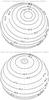 |
Fig. 3 Apparent Pluto temperatures, as viewed by a near-Sun observer in 2012, for a diurnal-only model with thermal inertia Γ = 25 MKS, Bond albedo = 0.46 and bolometric emissivity ϵb = 1. Top: surface temperatures. Bottom: temperatures at the bottom of the diurnal layer. |
4.3.2. Seasonal models
The above approach does not consider the impact of thermal inertia on seasonal timescales. Continuing with a Bond albedo of 0.46 and bolometric emissivity ϵb = 1, we show in Fig. 4 the seasonal temperature fields for two different values of the thermal inertia, Γ = 25 MKS and 3162 MKS. The first value, equal to that considered above for diurnal-only models, represents the situation of no thermal inertia gradient with depth. The second value represents one of the high thermal inertia cases favored by some of the recent climate models (Young 2012, 2013; Olkin et al. 2015). In Fig. 4, the left panels show the 2D (time, season) diurnally averaged (i.e., subdiurnal) surface temperatures; the right panels, which pertain to the epoch of the Herschel observations, show the latitudinal profile of: (i) this diurnally averaged temperature; (ii) the “deep” temperature (i.e., the temperature much below the seasonal skin depth); and (iii) the minimum value in the seasonal temperature vertical profile at each latitude. For the low thermal inertia (Γ = 25 MKS) case, seasonal effects on the diurnally averaged surface temperature are small. The temperature profile shown in the top right panel of Fig. 4 closely matches the subdiurnal temperature map of Fig. 3, except near and within the polar night where the zero temperatures of the diurnal-only model are replaced by more physical ~20 K−30 K values. In contrast, this model leads to rather cold temperatures of 30−36 K in the “deep” (i.e., subseasonal) subsurface, with minimum temperatures in the seasonal layer occasionnally falling below 30 K at high northern latitudes.
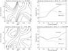 |
Fig. 4 Pluto temperatures from a seasonal model with thermal inertias Γ = 25 MKS (top) and 3162 MKS (bottom). A Bond albedo of 0.46 and bolometric emissivity ϵb = 1 are used. Left: “surface” temperature fields over a Pluto orbit. The dashed line indicates the epoch of the Herschel observations. Right: temperatures as a function of latitude for early March 2012. “Surface” and “deep” indicate temperatures at the top and bottom of the seasonal layer. “Minimum” refers to the minimum temperature within the seasonal layer for each latitude. |
The high (Γ = 3162 MKS) thermal inertia case5 has a much more dramatic effect on the diurnally averaged surface temperatures, which now show strongly subdued latitudinal contrasts of ~3 K for south pole to north pole at the Herschel epoch. In this situation, the deep temperatures reflect the mean insolation over the entire orbit and are almost hemispherically symmetric with maxima at the poles, minima near ±30° latitude, and a secondary maximum near the equator. These deep temperatures are in the range 38 K−39.5 K, and the minimum vertical temperature never falls below 37 K.
4.3.3. Comments and implications for the origin of low brightness temperatures
The temperatures shown in Figs. 3 and 4 are likely to be lower limits to the temperatures relevant to the Herschel observations for a number of reasons. First, they were calculated for a bolometric emissivity of 1.0, which, if anything, minimizes the calculated temperatures. Second, the geometric albedo that has been used is the Pluto-average value. Because the brightest regions are typically associated with N2 ice, the non-N2 ice regions are darker and thus warmer than the calculation indicates. Third, the above calculations do not include any increase of the effective emitting temperature due to roughness (those effects were incorporated in the form of a “thermophysical model beaming factor” in Lellouch et al. 2000a, 2011). Finally, while the Herschel beam encompasses Pluto and Charon, the above calculations pertain to Pluto only. Charon, which is slightly darker than Pluto, and based on the Spitzer 24 μm data likely to have a slightly smaller thermal inertia in the diurnal layer (Paper I), should therefore be warmer than Pluto on its dayside. This argument cannot be applied to the seasonal models however, as the relative seasonal thermal inertias of Pluto and Charon are unknown.
Yet, the temperatures shown in Figs. 3 and 4 are only relevant to the Pluto units not covered by N2 ice. The heat budget of the latter is dominated by sublimation-condensation exchanges, which, at a given point in time, maintain N2 to an isothermal state over the globe and the surface pressure to an essentially constant value (except for topographic effects) that is buffered by the N2 ice temperature (Young 2012). The most recent volatile transport models (Young 2012, 2013; Olkin et al. 2015; Hansen et al. 2015) indicate N2 ice temperatures constantly above 34 K throughout a Pluto year according to Hansen et al. (2015), and in the range 37.5−39.5 K according to Olkin et al. (2015), with T(N2) ~ 38.5 K in 2012. The surface pressure determination from New Horizons is ~10 μbar in July 2015 (Stern et al. 2015), corresponding to equilibrium at 37.0 K (Fray & Schmitt 2009). Because N2 is horizontally isothermal (i.e., does not show any diurnal temperature variation), it must also be vertically isothermal, at least over the diurnal skin depth. A firm lower limit of the N2 temperature is provided by the shape of the (2−0) band at 2.15 μm, which clearly indicates that N2 is in the β phase (Tryka et al. 1994), i.e., above the transition to cubic α phase at 35.6 K (Scott 1976; Trafton 2015). All of this suggests that regions covered with N2 ice are also warmer, albeit not necessarily by much, than the mean 500-μm TB that we measure (35 K, Fig.1).
The above considerations show that in most situations physical temperatures at the surface and in the subsurface of Pluto and Charon are considerably higher than the observed system brightness temperatures at 500 μm and beyond. The exception is the case of the subseasonal temperatures for the case of low seasonal thermal inertia (25 MKS, i.e., comparable to the diurnal seasonal thermal inertia), which can be as low as 27−36 K (Fig. 4). We conclude that the low observed TB do not result from the temperature gradient (colder at depth on the dayside) in the diurnal layer, but could conceivably be due to long-wavelength radiation probing a significant portion of the seasonal layer. This situation would require that (i) the seasonal thermal inertia is small, i.e., there is no significant vertical gradient of the thermal inertia; and (ii) the surface material is transparent enough that thermal radiation probes several meters below the surface.
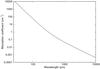 |
Fig. 5 Absorption coefficient of H2O ice, extrapolated to 50 K (see text for details). |
Estimates of Pluto’s seasonal inertia have been obtained from climate models (Hansen & Paige 1996; Young 2013; Hansen et al. 2015; Olkin et al. 2015) designed to match the atmospheric pressure evolution witnessed since 1988 and constraints on Pluto’s albedo distribution based on HST measurements. In addition to thermal inertia, these models include free parameters, such as the albedos and bolometric emissivities of the N2 frost and the involatile substrate, and the amout of volatile inventory. Once tuned to the pressure measurements, these models can also predict the orbit-long evolution of Pluto’s atmosphere. The latest two models, published prior to the New Horizons encounter, which give different priorities on the constraints to fit, differ rather radically in their conclusions with contrasting best-fit solutions for the seasonal thermal inertia (10−42 MKS in Hansen et al. (2015) vs. 1000−3162 MKS for Olkin et al. 2015) and diverging conclusions as to the fate of the atmosphere in the upcoming decades. The analysis of New Horizons data, particularly polar night temperatures with REX, should ultimately sort out this issue, but for now, we regard the seasonal thermal inertia of Pluto as significantly underconstrained.
However, even if the seasonal thermal inertia is small (i.e., comparable to the thermal inertia in the diurnal layer), we believe that the sub-mm radiation does not probe a large fraction of the seasonal skin depth (estimated above to be 3.5 m for Γ = 25 MKS). This stems from our estimate of the absorption coefficients of ices present on Pluto surface, on which we now elaborate. For N2 ice and CH4 ice, Lellouch et al. (2000a) presented absorption coefficients over 30−300 μm based both on early laboratory data compiled by Stansberry et al. (1996a) and on new optical constants measurements. These measurements (see Fig. 8 of Lellouch et al. 2000a) indicate typical absorption coefficients of ~0.5 cm-1 for N2 ice and ~1 cm-1 for CH4 ice, i.e., penetration depths of 2 cm and 1 cm, respectively, which is much shallower than the above value of the seasonal skin depth. The significance of these penetration depths is actually uncertain because the volatile ices might actually be restricted to an even thinner surface veneer.
H2O ice on Pluto has long escaped spectroscopic detection, and based on initial New Horizons data appears to be exposed only in a number of specific locations, usually associated with red color, suggestive of water ice/tholin mix (Grundy et al. 2015; Cook et al. 2015). Nonetheless, water ice is likely to be ubiquitous in Pluto’s near subsurface, given its cosmogonical abundance, Pluto’s density, and its presence on Charon’s surface6. Absorption coefficients for pure water ice (kH2O) at sub-mm-to-cm wavelengths are discussed extensively by Mätzler (1998), who also provides several analytic formulations to estimate them as a function of frequency and temperature along with illustrative plots. We use the Mishima et al. (1983) formulation (see Appendix of Mätzler 1998). Its applicability is normally restricted to temperatures above 100 K, but Fig. 2 of Mätzler (1998) indicates the trend with temperature. Absorption coefficients extrapolated to 50 K (estimated as half the values at 100 K) are shown in Fig. 5. At 500 μm, our best estimate is kH2O = 0.25 cm-1, comparable to the above values for CH4 and N2 ices. The corresponding penetration length is therefore comparable to the diurnal skin depth but remains negligible compared to the seasonal skin depth, even for seasonal Γ = 25 MKS. According to these calculations, the seasonal layer would be probed only at a wavelength of ~4 mm and beyond. We also remark that the expression from Mishima et al. (1983) would give a penetration depth of 56 m at 2.2 cm, which is an order of magnitude larger than indicated by the laboratory measurements of Paillou et al. (2008). In addition, small concentrations of impurities can dramatically reduce the microwave transparency of water ice (e.g., Chyba et al. 1998 and references therein). Therefore, the above calculations likely indicate upper limits to the actual penetration depth of radiation in a H2O ice layer, from which we conclude that the seasonal layer is not reached at the Herschel wavelengths.
We conclude that the low brightness temperatures observed at the longest Herschel wavelengths cannot be explained by subsurface sounding, and imply emissivity effects. In what follows, we present models aimed at fitting the Herschel light curves to evaluate the mean spectral emissivity of the Pluto-Charon system.
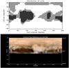 |
Fig. 6 Top: adopted Pluto units for modeling (white = N2, gray = CH4, black = H2O/tholin). Bottom: map of Pluto created from images taken from June 27 to July 3 by the Long Range Reconnaissance Imager (LORRI) on New Horizons, combined with lower resolution color data from the spacecraft’s Ralph instrument7. Cthulhu Regio is the dark region covering ~30°E-160°E longitudes. Sputnik Planum is the southern part of the bright region immediately to the east (informal names are taken from Stern et al. 2015). |
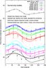 |
Fig. 7 Fits of the Spitzer 2004 (black points at top) and Herschel 2012 (all other points) brightness temperatures of the Pluto-Charon system using a diurnal-only model. Thin dotted lines: Spitzer-derived model (case 1 in Table 2). Dashed lines: Spitzer-derived model with CH4 emissivities adjusted (case 2). Solid lines: new model (see text), assuming that radiation originates at the surface at all Herschel wavelengths (case 4). Dashed lines: same, but assuming that radiation originates in the subdiurnal layer at all Herschel wavelengths (case 5). |
 |
Fig. 8 Fits of the Spitzer 2004 (black points at top) and Herschel 2012 (all other points) brightness temperatures of the Pluto-Charon system using a seasonal+diurnal model. The seasonal thermal inertia is 2000 MKS. Solid lines: model assuming that radiation originates at the surface at all Herschel wavelengths (case 4b in Table 2). Dashed lines: same, but using the wavelength-dependent absorption coefficient from Fig. 5 (case 6b). |
4.4. Fit of Herschel data
Using the above thermophysical models, we expand upon the models developed previously for fitting the ISO and Spitzer data (Lellouch et al. 2000a, 2011). Briefly, these models described the Pluto-Charon system as composed of four units (N2 ice, CH4 ice, H2O/tholin mix, and Charon), with specific distributions and geometric and bolometric albedos constrained by Pluto’s optical light curve, permitting one to calculate the thermal radiation (assumed Lambertian) of the entire system. The distribution of surface units was based on visible imaging and photometry (HST, mutual events) and near-infrared Earth-based spectroscopy. To calculate the local surface temperatures, a diurnal-only thermophysical model was used for all four units except N2 ice, which was maintained at a fixed N2 frost temperature. Another special condition was that the CH4 temperature was allowed to vary in accordance to thermophysical model predictions, but was capped at a maximum 54 K temperature to account, in a simplified manner, for sublimation cooling effects for CH4, which become important above this temperature (Stansberry et al. 1996b).
This “end-member” description is obviously outdated by the high-resolution New Horizons/LORRI imaging results (Stern et al. 2015), but until high-resolution maps of composition and albedo from LORRI and Ralph are available, it remains the only practical approach for our purpose. For now, we only considered the distribution favored in Paper I (“g2”, their Fig. 4), remarking its rather nice consistency with the early LORRI/images (Fig. 6). Furthermore, this distribution is also roughly consistent with early compositional results from New Horizons/Ralph , which show both N2 and CH4 in Sputnik Planum, neither N2 nor CH4 in Cthulhu Regio, CH4 north of Cthulhu and in the north polar region, and N2 at mid-northern latitudes (Grundy et al. 2015; L. Young, priv. comm.). The model free parameters are the thermal inertias of Pluto and Charon (expressed in terms of the thermal parameter Θ 8), plus the bolometric and/or spectral emissivity of some of the units, especially CH4 ice. Fitting the Spitzer 2004 light curve makes it possible to estimate the thermal inertias of Pluto and Charon separately because the former primarily dictates the 24 μm light-curve amplitude, while the latter determines the large contribution of Charon to the observed mean 24-μm TB (see Paper I for details).
We start by testing the best-fit model of Paper I determined from the Spitzer 2004 data. In this diurnal-only model, the spectral and bolometric emissivity of Charon and of the H2O/tholin unit of Pluto were fixed to 1. Inferred parameters were the thermal parameters of Pluto and Charon, ΘPL = 6 (i.e., ΓPL = 22 MKS) and ΘCH = 4.5 (ΓCH = 22 MKS); bolometric emissivity of methane, ϵb,CH4 = 0.7; and spectral emissivity of methane, ϵCH4 = 0.7, 0.6, and 0.45 at 70, 100, and 160 μm, respectively. As indicated by the thin dotted lines in Fig. 7, this model (case 1 in Table 2), which provides an excellent fit of the Spitzer 2004 data, is inconsistent with the Herschel measurements as it yields brightness temperatures that are too low at 100 and 160 μm, as well as too much light-curve contrast at these wavelengths. The first deficiency largely results from the poor quality of the Spitzer 2004 156 μm measurements. These measurements, which are now shown to be inconsistent with other data (Fig. 2), unduly skewed the model toward brightness temperatures that are too low. This deficiency can be corrected for by adjusting the CH4 ice spectral emissivities (to 0.67, 0.80, 0.84, 0.58, 0.53, and 0.43 at 70, 100, 160, 250, 350, and 500 μm, respectively; case 2 in Table 2). However the synthetic light curves (long dashed-lines in Fig. 7) still have too much contrast, except at 70 μm. This implies that the other units besides CH4 ice are also subject to wavelength-dependent emissivities. Relaxing the hypothesis that the spectral emissivity of Charon and of the H2O/tholin units are equal to unity, we searched for the spectral emissivity (now assumed for simplicity to be the same for Charon and the three Pluto units) that permits a fit to all light curves (case 3 in Table 2). This case permits a good fit (not shown in Fig. 7) to the data, but we do not regard it as satisfactory because the associated Planck-averaged bolometric emissivity is 0.82−0.85, which is inconsistent with the bolometric emissivities prescribed for the tholin/H2O, CH4 and Charon units (1.0, 0.7, and 1.0, respectively).
The above results point to the need to revise the Spitzer-derived models, and we here updated the fitting approach. For the sake of simplicity, we adopted fiducial bolometric emissivities of 0.90 for Charon and all Pluto units (for N2 ice, the bolometric emissivity is not explicitly used; instead a uniform temperature is specified). We also do not include a “beaming factor” in the thermophysical model (as was done in Paper I), i.e., we ignore surface roughness effects; these are discussed separately later. With these changes to the model, the Spitzer-2004 24 μm light curve was refit in terms of separate thermal parameters for Pluto and Charon at the Spitzer epoch, adopting a 24 μm emissivity of 1.0 for all units. Best-fit ΘPL = 7 and ΓCH = 3 values (i.e., ΓPL = 26 MKS and ΓCH = 14 MKS) were obtained. The thermophysical model was then re-run for the 2012 conditions, searching for the spectral emissivities (again assumed to be the same for all units) that permitted to fit the ensemble of Herschel light curves. Because there is considerable uncertainty in the penetration length of the far-IR radiation, we considered three cases: (i) small penetration at all six Herschel wavelengths, i.e., the surface itself is probed (case 4); (ii) large penetration, i.e., the subdiurnal layer is probed (case 5); and (iii) a wavelength-dependent absorption coefficient, following Fig. 5 (case 6). The required spectral emissivities for cases 4−6 are given in Table 2 and the associated emissivity curves are shown in Fig. 9. The overall fits of the thermal data for cases 4 and 6 are shown in Fig. 7 with solid and dashed-dotted lines, respectively.
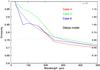 |
Fig. 9 Derived emissivities for models 4−6 (see text and Table 2). These emissivities are compared to predictions for a smooth surface with dielectric constants indicated on the right y scale (the dotted line is for a dielectric constant of 3.10) and for a Debye model with ϵs = 5, ϵ∞ = 1 and νr = 10cm-1 (see text). |
Cases 4, 5, and 6 imply Planck-averaged bolometric emissivities of 0.83−0.86, 0.89−0.93, and 0.83−0.86. Although this is not precisely consistent with the adopted bolometric emissivities of 0.90, and although these models provide a somewhat worse fit to the 24 μm data than do the “Spitzer-only” models, we consider that the overall solution is physically satisfactory, and that Fig. 9 provides a proper estimate of the spectral emissivity behavior of the Pluto-Charon system as a whole.
The above results pertain to diurnal-only models. To study the effect of a large seasonal thermal inertia on the derived emissivities, cases 3 to 6 were reconsidered assuming that the subdiurnal temperature is determined by a seasonal thermal inertia of 2000 MKS (for both Pluto and Charon). Solution cases in terms of the diurnal thermal inertias and spectral emissivities are given in Table 2 (cases 3b to 6b). Since the large seasonal thermal inertia implies cold subdiurnal temperatures, somewhat smaller thermal inertias (compared to the diurnal-only case) are required to fit the Spitzer 24 μm fluxes. Furthermore, these subdiurnal temperatures are in this case too cold (see also Fig. 4) to fit the Herschel 70, 100, and 160 μm TB, making this case (case 5b) not viable. In contrast, cases 3b, 4b, and 6b have emissivity solutions insignificantly different from corresponding cases 3, 4, and 6 (Table 2). Fits of the Spitzer 24 μm and Herschel data with these seasonal + diurnal models (cases 4b and 6b) are shown in Fig. 8. They are almost indistinguishable from those shown in Fig. 7. Thus (and not surprisingly given that all our data pertain to nearly the same season), we are unable to constrain the seasonal thermal inertia from our data. Nonetheless, the ensemble of model solutions (Table 2) yields diurnal thermal inertias ΓPL = 16−26 MKS and ΓCH = 9−14 MKS, confirming results from Paper I.
Emissivity models.
Model predictions for Case 4 of Table 2 over 20−1000 μm, calculated for the geometric conditions of September 2004 (subsolar latitude = 34.5°, heliocentric distance = 32.19 AU), are superimposed on Fig. 2 (gray dotted line). Although the figure gathers data with different subsolar latitudes, the fit shows the overall model adequacy. We do not attempt to fit the disparate set of sub-mm/mm data, noting that much improved constraints at these wavelengths are expected from ALMA (Butler et al. 2015). The same model, but in which spectral emissivities are forced to unity, is shown for comparison (blue dotted line). This latter case still shows a decrease of the brightness temperatures with wavelength as a result of the mixing of different surface temperatures (see Sect. 4.2), but this effect is clearly not sufficient to explain the data.
In a recent study, Trafton (2015) questioned the paradigm interpretation of Pluto’s near-infrared spectrum in terms of “pure” and “diluted” CH4 ice, and, on thermodynamical grounds, proposed an alternate surface scenario with the mixture of areas covered by N2-rich (N2:CH4, saturated with CH4) and CH4-rich (CH4:N2, saturated with N2) solid solutions. For each unit, saturation of the secondary component occurs at the several percent level (about 3% at 37 K; see Table 1 of Trafton 2015). The CH4:N2 unit would correspond optically to what has been reported as “pure CH4”, but with the key difference that this CH4:N2 unit would be isothermal because of the role of the N2-rich ice in transporting latent heat between solid solutions. As suggested by Trafton, thermal measurements may provide a test of these ideas. Coming back to the diurnal-only model (case 4 in Table 2) we attempted to remodel the Spitzer 24 μm light curve (best suited for this task because of its enhanced sensitivity to temperatures) under the assumption that the “CH4 ice unit” is actually isothermal at some constant temperature TCH4. As can be seen in Fig. 12 of Lellouch et al. (2011), the contribution of the CH4 unit is most important over L = 280−30 (and responsible for the increase of flux with increasing longitude in this range). If the other components (Charon and tholin/H2O mix) are left untouched, the range of brightness temperatures measured in this longitude bin requires TCH4 = 51−52 K, though the fit is not as good as it is with variable temperatures. Allowing for an increase in the contribution of the tholin/H2O or Charon unit (i.e., decreasing their thermal inertia) makes room for slightly lower values of TCH4 (~50 K), but the shape of the calculated light curve degrades unacceptably below this temperature. We conclude that the 24 μm light curve measured by Spitzer (i) implies that if the “CH4 ice unit” actually represents isothermal CH4-rich CH4:N2 mixtures, these must be at least 50 K warm, i.e., much warmer than the N2-rich areas (~37 K); and (ii) favors spatially and diurnally variable temperatures for the CH4-dominated areas over the isothermal case. At face value, these conclusions do not support Trafton’s (2015) scenario of isothermal CH4:N2 at the same temperature as N2:CH4, although reconciliation might be possible if regions attributed to pure CH4 actually represent a spotty coverage of CH4:N2 solutions at 37 K with nonvolatile material. Finally, at 50 K, the saturated N2 abundance in CH4:N2 would be 2−3 times larger than at 37 K.
5. Discussion
5.1. Roughness effects?
The emissivities derived in this work (Table 2, Fig. 9) either make use of a simple treatment of surface roughness in the case of the “Spitzer-only” models (cases 2 and 3 in Table 2) or ignore roughness (cases 4, 5, 6, 4b, 6b). As reviewed, e.g., in Keihm et al. (2013) and Delbo et al. (2015), disk-integrated infrared measurements of airless bodies have long indicated flux enhancements in near zero-phase angle observations relative to thermophysical models of smooth surfaces (even if zero thermal inertia is used in these models). These flux enhancements, strongest at shorter thermal wavelengths, are commonly viewed as the effect of small-scale surface roughness. The latter results in a multiplicity of surface temperatures at any scale with an enhanced contribution of the hottest temperatures to the flux, particularly at shorter wavelengths. These effects led to the introduction of the “beaming factor” in the literature (e.g., Lebofsky et al. 1986; Harris 1998; Delbo et al. 2015), whereby a semiempirical correction to the thermophysically calculated surface temperatures can be applied to match the infrared fluxes. While this approach is usually appropriate for fitting disk-averaged observations in terms of an object’s diameter and albedo, it becomes insufficient when dealing with multiwavelength, multiphase angle, and/or multi local-time data. Examples of its shortcomings have been demonstrated, for example, by comparing its predictions of center-to-limb temperature profiles to those of physical roughness models constrained by lunar thermal emission profiles (Rozitis & Green 2011). Other evidence of thermal emission enhancements not amenable to a single “beaming factor” was obtained from spectral images of comets 103P/Hartley 2 and 9P/Tempel 1 (Groussin et al. 2013) at thermal wavelengths. These data indicate color temperatures that are barely dependent on incidence angle i, vastly exceeding predictions from smooth surface models at large values of i. This is interpreted by the fact that thermal emission from a given region of a comet is dominated by facets that are oriented toward the Sun with a temperature that is mostly independent of the “smooth” incidence angle, but instead strongly dependent on local topography (slopes, projected shadows) on sub-km to sub-mm scales. In Groussin et al. (2013), these effects were modeled by replacing the Planck function B(λ, T) by a product Λ × B(λ, T), where T is the color temperature and Λ (<1) represents in essence the fraction of an observed region that undergoes the highest temperatures, as measured by T. The Λ parameter was found to decrease with increasing incidence angle, as expected for progressively larger effects of projected shadows.
In many asteroid thermal models, macroscopic roughness (e.g., occurring on scales larger than the thermal skin depth) is usually described by crater models, accounting for effects of partial shadowing, scattering of sunlight, mutual radiative heat exchanges within depressions, using different approximations and methods of coupling with heat conduction. Key parameters are the crater surface coverage and depth-to-diameter ratio, which combine to define the surface “rms slope”. For example, Lagerros (1998) found that high roughnesses (rms slope ~35°) are required to mimic, in a flux-averaged sense, the standard beaming factor for asteroids. Based on the crater formulation from Hansen (1977), Keihm et al. (2013)’s calculations for a typical 0.15 albedo asteroid at 2.5 AU with low thermal inertia indicate that large roughnesses (50% coverage of hemispherical craters) produce flux enhancements (over the smooth surface case) by ~9% at 100 μm, but as much as ~40% at 12 μm (see their Fig. 1)9 and even more at shorter wavelengths. These calculated flux enhancements can be applied to other objects by noting that they are unique functions of λ × T by virtue of the Planck function dependence. “Transposing” a 0.15 albedo asteroid at rh = 2.5 AU (which has an instantaneous subsolar temperature of TSS = 246.0 K for ϵ = 0.9) to Pluto (A = 0.46, rh = 32.2 AU, giving TSS = 61.2 K), means that for equal roughness the same flux enhancements would occur for Pluto over 48 μm−400 μm. Although the case described by Keihm et al. (2013) presumably represents an upper limit of any realistic roughness for Pluto, the above comparison might suggest that wavelength-dependent roughness effects may affect the Spitzer+Herschel fluxes at typical levels of a few tens of percent. While the enhancements due to roughness are wavelength-dependent when considered in flux, they in fact imply approximately constant increases in brightness temperatures. Specifically, when reference is made to a smooth equilibrium model (EQM), the above flux enhancements for the considered asteroid imply brightness temperatures increases of 14−15 K over 12−100 μm. Rescaling to the Pluto case would mean that the 48 μm−400 μm TB could be affected by roughness effects at the 3−4 K level at most with essentially no spectral dependence10. This is a small fraction of the observed TBs decrease (~15 K) over that interval (Fig. 2). The potential 3−4 K effect is even dwarfed by the 10 K TB difference associated with a spectral emissivity of ~0.7, as we find required by the 500 μm TB (Table 2). Finally and most importantly, and as alluded to in Sect. 4.3.3, since surface roughness can only enhance disk-averaged fluxes, any significant effects would actually exacerbate (by a few K) the fact, outlined in Sect. 4.3, that the long-wavelength TB are below any plausible temperatures within Pluto’s subsurface. We are left to conclude that roughness effects are not the cause of the emissivity spectral dependence that we observe.
5.2. Comparison to other bodies and interpretation
Modeling of the Herschel data has led us to (i) an updated estimate of the Pluto and Charon diurnal thermal inertias, and (ii) an assessement of their spectral emissivities over 20−500 μm. We determine ΓPL = 16−26 MKS and ΓCH = 9−14 MKS, in good agreement from inferences based on Spitzer-only data (Paper I), namely ΓPL = 20−30 MKS and ΓCH = 10−150 MKS (with most solutions calling for ΓCH = 10−20 MKS). These thermal inertias are low compared to those of compact ices, but still factors-of-several higher than the value statistically determined for the TNO population (Γ = 2.5 ± 0.5 MKS, Lellouch et al. 2013b). As discussed in that paper, the difference does not necessarily imply intrinsically different thermal surface properties. For equal density and conduction properties, the diurnal skin depth at Pluto/Charon (P = 6.387 day) is ~5 times larger than that of a typical TNO with an 8-h rotation period; hence the difference between Charon and a typical TNO might simply be consistent with an approximately linear increase of the thermal inertia with depth. The apparently higher thermal inertia at Pluto vs. Charon may be related to atmospheric-assisted conduction in a porous surface (Lellouch et al. 2000a).
The very large (>30%) decline of the Pluto-Charon brightness temperatures from ~20 to 500 μm, and probably beyond, is partly caused by the mixing of different temperatures on regional scales. The main conclusion of our work is that, once this is taken into account, the reminder of the effect is not caused by surface roughness or subsurface sounding at the longest wavelengths, so that “genuine” emissivity spectral dependence occurs. This conclusion confirms and expands that reached for the 1.2 mm emission of the Pluto-Charon system (Lellouch et al. 2000b).
Low emissivities at long wavelengths have been observed on a number of solar system icy bodies. Muhleman & Berge (1991) reported 3−40 mm flux measurements of Europa and especially Ganymede indicating brightness temperatures well below the subdiurnal temperature, confirming earlier results from De Pater et al. (1984). Using Cassini/RADAR, Ostro et al. (2006) determined 2.2 cm brightness temperatures of several Saturn satellites. When comparing these brightness temperatures to the “isothermal equilibrium temperature” (i.e., the mean equilibrium surface temperature over a sphere), this implied averaged emissivities as low as 0.44 for Tethys, 0.59 for Enceladus and Rhea, and 0.69−0.81 for Iapetus. A 0.6−0.7 emissivity was also found at Enceladus by Ries & Janssen (2015). However, these estimates did not include the effect of subsurface sounding. Focusing on Iapetus, but using a thermophysical modeling including subsurface sounding, Le Gall et al. (2014) determined slightly higher emissivities (0.78−0.87, depending on the regions), but still significantly below unity. Also at Iapetus, Ries (2012) determined an extraordinarily low 9 mm effective emissivity (~0.3−0.4) on the trailing side. Emissivity effects are also seen in millimeter-wavelength measurements of various kinds of ice and snow on Earth (Hewison & English 1999).
Fewer emissivity measurements are available in the far-IR (as opposed to sub-mm/cm wavelengths). From ISO/LWS observations of Mars, Burgdorf et al. (2000) inferred a spectral emissivity declining from 0.97 at 50 μm to 0.92 at 180 μm. Using Herschel, Leyrat et al. (2012) inferred a large decrease of the spectral emissivity of asteroid 4 Vesta, from 0.9 at 70 μm to 0.7 at 500 μm, essentially confirming previous findings by Müller & Lagerros (1998). These analyses, however, while including a detailed surface temperature model, did not account for possible subsurface sounding effects. Evidence for a spectrally-decreasing emissivity was also found for several Kuiper Belt and Centaurs by Fornasier et al. (2013) from combined Spitzer/MIPS, Herschel/PACS, and Herschel/SPIRE data. Although once again, this work did not explicitly include vertical temperature profiles, a striking observational fact was the abrupt fall-off of the emitted fluxes beyond 300 or 400 μm, with most objects not detected at 500 μm.
Our results for Pluto-Charon add further evidence that unlike dust/rock regolith asteroids (Keihm et al. 2013), icy solar system surfaces show long-wavelength emissivity effects not amenable to a combination of surface roughness and subsurface sounding. Reasons for lower-than-unity emissivities may include (i) dielectric constants larger than 1, implying reflection of the upward thermal radiation at the surface interface; (ii) particle scattering, which produces an emissivity minimum for particle sizes comparable to λ/4π; and (iii) volume scattering, whereby the combination of a weakly-absorbing medium down to the electrical skin depth and inhomogeneities or voids on scales comparable or larger than the wavelength causes internal reflections (Ostro et al. 2006; Le Gall et al. 2014). Volume scattering is commonly invoked as the dominant scattering mechanism at microwave (mm-cm) wavelengths (Janssen et al. 2009; Le Gall et al. 2014; Ries & Janssen 2015).
In the measurements of Hewison & English (1999), the ice/snow emissivity dependence with frequency varies with the age, wetness, surface state, and transparency of the ice as a result of the combination of dielectric and scattering effects. This was modeled in a semiempirical way using a Debye-like form of the complex permittivity,  from which Fresnel coefficients can be calculated as a function of incidence angle. Here ϵs is the effective static permittivity, ϵ∞ its high-frequency limit and νr is the effective relaxation frequency. This parameterization handles both dielectric surfaces (by setting ϵs>ϵ∞) and volume scattering (ϵs<ϵ∞), and both behaviors are found in terrestrial icy material. Adopting the above parameterization, and assuming a smooth surface and an equal mix of the two polarizations when calculating the Fresnel coefficients, the spectral dependence we derive for Pluto-Charon’s emissivity can be approximately fit with ϵs = 5, ϵ∞ = 1, and νr = 10 cm-1 (Fig. 9). The values of ϵs and ϵ∞ encompass that of the water ice dielectric constant (3.10−3.13 at 50−100 K; Gough 1972; Paillou et al. 2008), for which a ~0.76 constant spectral emissivity would be expected. Nonetheless, the above should be seen primarily as a working empirical model, and ϵs>ϵ∞ suggests that volume scattering may not be important in causing the depressed emissivities over 70−500 μm. In fact, as the volume scattering process operates in the electrical depth layer and for voids/inhomogeneities larger than the wavelength, it cannot be important when the absorption coefficient becomes smaller than the inverse of the wavelength, i.e., below 100 μm for H2O ice.
The emissivity decrease with wavelength, possibly extending toward the mm range, may also indicate particle scattering with a typical particle size of at least 100 μm. Stansberry et al. (1996a) performed emissivity calculations for N2 ice and CH4 ice with various grain sizes, based on Hapke theory (Hapke 1993) and their far-IR absorption properties. Their results do indicate significantly less than unity far-IR emissivities, but the spectral behavior, with an emissivity decrease occurring only longward of 50 μm for CH4 and 150 μm for N2, is not consistent with the mean emissivity behavior we infer here. A similar problem was noted in Paper I, where the high 24 μm emissivity inferred for CH4 ice was inconsistent with the calculations of Stansberry et al. (1996a) for a broad range of grain sizes. Calculations for H2O ice are not available but the similarity of its absorption coefficient to that of N2 and CH4 ice at ~300 μm (about 1 cm-1) indicates that IR emissivities lower than unity are to be expected. Notwithstanding with the above issues, we conclude that the mean emissivity curve we have derived likely results from the combination of a high dielectric constant and particle scattering in relatively transparent surface ices.
The temperature of Pluto’s N2 ice can be inferred from the atmospheric pressure. The buffering temperature of a 10 μbar N2 atmosphere (Stern et al. 2015) is 37.0 K (Fray & Schmitt 2009). An expression for the globally constant temperature of the N2 ice (TN2) can be found in Stansberry & Yelle (1999) as a function of γ, the ratio of the total area of N2 ice to its cross-sectional area as viewed from the Sun. For ubiquitous N2 frosts (and many other reasonable surface ice configurations), γ = 4, and TN2 = TSS/ . For rh = 32.9 AU (July 2015), TN2 = 37.0 K implies a relationship between the Bond albedo (Ab) and bolometric emissivity, namely (1−Ab)/ϵb = 0.335. For the N2 ice unit of the assumed terrain distribution (“g2”), Paper I derived a geometric albedo of 0.73, and assumed a phase integral of 0.90, yielding Ab = 0.657. With a bolometric emissivity ϵb = 0.9 as we advocate here, this yields (1−Ab)/ϵb = 0.381. The agreement with the above value is only approximate but could be brought to perfection with very small changes, e.g., using γ = 4.5 instead of 4 or a phase integral of 0.96 instead of 0.90. Furthermore, our nominal value of 0.381 matches well the range of solutions derived from the climate models (Young 2013; Hansen et al. 2015). Indeed, restricting the discussion to models that best approach a ~10 μbar pressure in 2015 (cases PNV21-23 and EPP14 from Young 2013, and models #55 and #66 from Hansen et al. 2015), these models all converge to (1−Ab)/ϵb in the range 0.363−0.375. Thus, it appears that there is no major difficulty with a N2 bolometric emissivity of 0.9. The heat budget for N2 ice will be best revisited after results from photometric (albedos, phase integrals) investigations from New Horizons become available.
Although the New Horizons spacecraft does not carry a dedicated thermal radiometer, the Radio Experiment (REX) acquired measurements of the thermal emission from Pluto at 4.2 cm during two linear scans across the disk at close range including both day and night sides, and a third scan was obtained during the dark side transit of the occultation (Linscott et al. 2015). These data should provide crucial information on the surface temperature and its spatial variations, especially on the polar night temperature, which is the most diagnostic of thermal inertia on seasonal timescales (see Fig. 4). The present work suggests that emissivity effects will strongly impact the interpretation of these data.
The fits of the Herschel data presented here should still be viewed as preliminary. Future analyses making use of detailed surface maps based on New Horizons/Ralph (including albedo, composition and its vertical statigraphy, particle size, phase functions, and possibly temperatures from band shape) will be possible when those datasets become available (e.g., Grundy et al. 2015). More generally, the ISO, Spitzer, and Herschel combined Pluto-Charon light curves constitute a legacy dataset at thermal wavelengths, against which temperature predictions from seasonal climate models should be tested, which will be soon complemented by additional data. Rotationally resolved ALMA data separating Pluto from Charon are already available (Butler et al. 2015), and thermal maps at ~0.01′′ spatial resolution will be achievable in the coming years. Starting in 2018, the JWST/MIRI will measure Pluto and Charon emission over ~10−27 μm. These facilities will be invaluable to study the predicted evolution of the surface thermal properties as the Pluto system recedes from the Sun.
See also AOT Release Note: PACS Photometer Point/Compact Source Mode 2010, PICC-ME-TN-036, Version 2.0, custodian Th. Müller (PACS Photometer Point/Compact Source Mode 2010).
It can be shown (see, e.g., Le Gall et al. 2014 and Schloerb et al. 2015 for recent applications) that the outgoing thermal radiation depends on the ratio of the electric skin depth Le to the relevant thermal skin depth, rather than on their absolute values.
This ignores internal heating. A typical radiogenic heating of 2.4 erg cm-2 s-1 (Robuchon & Nimmo 2011) would yield a ~14 K polar night temperature for unit bolometric emissivity.
The choice of 3162 MKS in Young (2013) and Olkin et al. (2015) is just an effect of their thermal inertia grid, with two values per decade, for parameter searches. No physical inference should be drawn from the fact that 3162 MKS is higher than the thermal inertia for solid H2O at 40 K (2200 MKS, Spencer & Moore 1992).
Evidence for water ice bedrocks is also strongly suggested by the New Horizons discovery of several kilometer high topographic features on both Pluto’s and Charon’s surfaces (Stern et al. 2015).
Θ is related to the thermal inertia Γ by  , where ω = 2π/(6.3872 days) is the body rotation rate, ϵb is the bolometric emissivity of the surface, σ is Stefan-Boltzmann’s constant, and TSS is the instantaneous equilibrium temperature at the subsolar point,
Similar numbers are obtained from the crater model of Müller (2002).
For comparison, the “thermophysical beaming factor” used in Paper I was 0.905-0.925, corresponding to a typical ~1 K increase of the brightness temperatures.
Acknowledgments
PACS has been developed by a consortium of institutes led by MPE (Germany) and including UVIE (Austria); KU Leuven, CSL, IMEC (Belgium); CEA, LAM (France); MPIA (Germany); INAF-IFSI/OAA/OAP/OAT, LENS, SISSA (Italy); IAC (Spain). This development has been supported by the funding agencies BMVIT (Austria), ESA-PRODEX (Belgium), CEA/CNES (France), DLR (Germany), ASI/INAF (Italy), and CICYT/MCYT (Spain). SPIRE has been developed by a consortium of institutes led by Cardiff University (UK) and including Univ. Lethbridge (Canada); NAOC (China); CEA, LAM (France); IFSI, Univ. Padua (Italy); IAC (Spain); Stockholm Observatory (Sweden); Imperial College London, RAL, UCL-MSSL, UKATC, Univ. Sussex (UK); and Caltech, JPL, NHSC, Univ. Colorado (USA). This development has been supported by national funding agencies: CSA (Canada); NAOC (China); CEA, CNES, CNRS (France); ASI (Italy); MCINN (Spain); SNSB (Sweden); STFC, UKSA (UK); and NASA (USA). Additional funding support for some instrument activities has been provided by ESA. Data presented in this paper were analyzed using “HIPE”, a joint development by the Herschel Science Ground Segment Consortium, consisting of ESA, the NASA Herschel Science Center, and the HIFI, PACS, and SPIRE consortia. We are indebted to the ESA staff, in particular Rosario Lorente and Mark Kidger, for a flexible and flawless implementation of the observations. E.L., S.F., and R.M. were supported by the French Programme National de Planétologie. C.K. and G.M. were supported by the OTKA/NKFIH K-104607 grant of the Hungarian Research Fund/National Research, Development and Innovation Office; and the contract 4000109997/13/NL/KML of the Hungarian Space Office and the European Space Agency. Support for the work of S.P. was provided by NASA through an award issue by JPL/Caltech. We thank Leslie Young for constructive comments.
References
- Altenhoff, W. J., Chini, R., Hein, H., et al. 1988, A&A, 190, L15 [NASA ADS] [Google Scholar]
- Brucker, M., Grundy, W. M., Stansberry, J., et al. 2009, Icarus, 201, 284 [NASA ADS] [CrossRef] [Google Scholar]
- Butler, B., Gurwell, M., Lellouch, E., et al. 2015, 47th DPS meeting, 210.04 [Google Scholar]
- Burgdorf, M.J., Encrenaz, T., Lellouch, E., et al. 2000, Icarus, 145, 79 [NASA ADS] [CrossRef] [Google Scholar]
- Buie, M. W., Tholen, D. J., & Wasserman, L. H. 1997, Icarus, 125, 233 [NASA ADS] [CrossRef] [Google Scholar]
- Chyba, C. F., Ostro, S. J., & Edwards, B. 1998, Icarus, 134, 292 [NASA ADS] [CrossRef] [Google Scholar]
- Cook, J. C., Cruikshank, D. P., Dalle Ore, C. M. et al. 2015, 47th DPS meeting, 210.04 [Google Scholar]
- Delbo, M., Mueller, M., Emery, J. P., et al. 2015, ArXiv e-prints [arXiv:1508.05575] [Google Scholar]
- De Pater, I., Brown, R. A., & Dickel, J. R. 1984, Icarus 57, 93 [NASA ADS] [CrossRef] [Google Scholar]
- Fornasier, S., Lellouch, E., Müller, T., et al. 2013, A&A, 555, A15 [NASA ADS] [CrossRef] [EDP Sciences] [Google Scholar]
- Fray, N., & Schmitt, B. 2009, Planet. Space Sci., 57, 2053 [NASA ADS] [CrossRef] [Google Scholar]
- Gough, S. R. 1972, Can. J. Chem. 50, 3046 [Google Scholar]
- Griffin, M., Abergel, A., Abreu, A., et al. 2010, A&A, 518, L3 [Google Scholar]
- Groussin, O., Sunshine, J. M., & Feaga, L. M. 2013, Icarus, 222, 580 [CrossRef] [Google Scholar]
- Grundy, W. M., Buie, M. W., Stansberry, J. A, et al. 1999, Icarus, 142, 536 [NASA ADS] [CrossRef] [Google Scholar]
- Grundy, W. M., Schmitt, B., & Quirico, E. 2002, Icarus, 185, 486 [NASA ADS] [CrossRef] [Google Scholar]
- Grundy, W. M., Binzel, R. P., Cook, J. C., et al. 2015, 47th DPS meeting, 200.01 [Google Scholar]
- Gurwell, M. A., Butler, B., & Moullet, A. 2011, EPSC-DPS Joint Meeting 271 [Google Scholar]
- Hansen, O. L. 1977, Icarus, 31, 456 [NASA ADS] [CrossRef] [Google Scholar]
- Hansen, C. J., & Paige, D. A. 1996, Icarus, 120, 247 [NASA ADS] [CrossRef] [Google Scholar]
- Hansen, C. J., Paige, D. A., & Young, L. A. 2015, Icarus, 246, 183 [NASA ADS] [CrossRef] [Google Scholar]
- Hapke, B. W. 1993, Theory of reflectance and emittance spectroscopy (Cambridge: Cambridge Univ. Press) [Google Scholar]
- Harris, A. W. 1998, Icarus, 131, 291 [NASA ADS] [CrossRef] [EDP Sciences] [Google Scholar]
- Hewison, T. J., & English, S. J. 1999, IEEE Trans. Geosc. Remot. Sound., 37, 1871 [Google Scholar]
- Janssen, M. A., Lorenz, R. D., West, R., et al. 2009, Icarus, 200, 222 [NASA ADS] [CrossRef] [Google Scholar]
- Jewitt, D. C. 1994, AJ, 107, 372 [NASA ADS] [CrossRef] [Google Scholar]
- Keihm, S., Kamp, L., & Gulkis, S. 2013, Icarus, 226, 1186 [NASA ADS] [CrossRef] [Google Scholar]
- Kiss, Cs., Müller, T. G., Vilenius, E., et al. 2014, Exp. Astr., 37, 161 [Google Scholar]
- Lagerros, J. S.V. 1996, A&A, 310, 1011 [NASA ADS] [Google Scholar]
- Lagerros, J. S.V. 1998, A&A, 332, 1123 [NASA ADS] [Google Scholar]
- Lebofsky, L. A., Sykes, M. V., Tedesco, E. F., et al. 1986, Icarus, 68, 239 [NASA ADS] [CrossRef] [Google Scholar]
- Le Gall, A., Leyrat, C., Janssen, M. A., et al. 2014, Icarus, 241, 221 [NASA ADS] [CrossRef] [Google Scholar]
- Lellouch, E., Laureijs, R., & Schmitt, B. 2000a, Icarus, 147, 220 [NASA ADS] [CrossRef] [Google Scholar]
- Lellouch, E., Paubert, G., Moreno, R., & Schmitt, B. 2000b, Icarus, 147, 580 [NASA ADS] [CrossRef] [Google Scholar]
- Lellouch, E., Stansberry, J., Emery, E., et al. 2011, Icarus, 214, 701 (Paper I) [NASA ADS] [CrossRef] [Google Scholar]
- Lellouch, E., Santos-Sanz, P., Fornasier, S., et al. 2013a, EPSC conference, #2013-91 [Google Scholar]
- Lellouch, E., Santos-Sanz, P., Lacerda, P., et al. 2013b, A&A, 557, A60 [NASA ADS] [CrossRef] [EDP Sciences] [Google Scholar]
- Lellouch, E., de Bergh, C., Sicardy, B., et al. 2015, Icarus, 246, 268 [NASA ADS] [CrossRef] [Google Scholar]
- Leyrat, C., Barucci, A., Müller, T., et al. 2012, A&A, 539, A154 [NASA ADS] [CrossRef] [EDP Sciences] [Google Scholar]
- Linscott, I., Stern, A., Weaver, H., et al. 2015, 47th DPS meeting, 101.03 [Google Scholar]
- Mätlzer, C. 1998, In Solar System Ices, eds. B. Schmitt, C. de Bergh, & M. Festou (Kluwer Academic), 241 [Google Scholar]
- Marton, G., Kiss, Cs., Balog, Z., et al. 2015, A&A, 579, L9 [NASA ADS] [CrossRef] [EDP Sciences] [Google Scholar]
- Mishima, O., Klug, D. D., & Whalley, E. 1983, J. Chem. Phys., 78, 6399 [NASA ADS] [CrossRef] [Google Scholar]
- Muhleman, D. O., & Berge, G. L. 1991, Icarus, 92, 263 [Google Scholar]
- Müller, T. G. 2002, Meteor. Planet. Sci., 37, 1919 [Google Scholar]
- Müller, T. G., & Lagerros, J. S. V. 1998, A&A, 338, 340 [NASA ADS] [Google Scholar]
- Müller, T. G., Lellouch, E., Stansberry, J., et al. 2010, A&A, 518, L146 [NASA ADS] [CrossRef] [EDP Sciences] [Google Scholar]
- Nguyen, H. T., Schulz, B., & Levenson, L. 2010, A&A, 518, L5 [NASA ADS] [CrossRef] [EDP Sciences] [Google Scholar]
- Olkin, C. A., Young, L. A., Borncamp, D., et al. 2015, Icarus, 246, 220 [Google Scholar]
- Ostro, S. J., West, R. D., Janssen, M. A., et al. 2006, Icarus, 183, 479 [NASA ADS] [CrossRef] [Google Scholar]
- Ott, S. 2010, ASP Conf. Ser., 434, 139 [Google Scholar]
- Paillou, P., Lunine, J., Ruffié, G., et al. 2008, Geophys. Res. Lett., 35, L18202 [NASA ADS] [CrossRef] [Google Scholar]
- Pilbratt, G., Riedinger, J. R., Passvogel, T., et al. 2010, A&A, 518, L1 [CrossRef] [EDP Sciences] [Google Scholar]
- Poglitsch, A., Waelkens, C., Geis, N., et al. 2010, A&A, 518, L2 [NASA ADS] [CrossRef] [EDP Sciences] [Google Scholar]
- PACS Photometer Point/Compact Source Mode 2010, PICC-ME-TN-036, http://herschel.esac.esa.int/twiki/bin/view/Public/PacsCalibrationWeb?template=viewprint#Observing_with_PACS [Google Scholar]
- Quirico, E., & Schmitt, B. 1997, Icarus, 128, 181 [NASA ADS] [CrossRef] [Google Scholar]
- Redman, R. O., Feldman, P. A., & Matthews, H. E. 1998, AJ, 116, 1478 [NASA ADS] [CrossRef] [Google Scholar]
- Reuters, D. C., Sterm, S. A., Scherrer, J., et al. 2008, Space Sci. Rev., 140, 129 [NASA ADS] [CrossRef] [Google Scholar]
- Ries, P. 2012, Ph.D. Thesis, University of Virginia, USA [Google Scholar]
- Ries, P. A., & Janssen, M. 2015, Icarus, 257, 88 [NASA ADS] [CrossRef] [Google Scholar]
- Robuchon, X., & Nimmo, F. 2011, Icarus, 216, 426 [NASA ADS] [CrossRef] [Google Scholar]
- Rozitis, B., Green, S. F. 2011, MNRAS, 415, 2042 [NASA ADS] [CrossRef] [Google Scholar]
- Santos-Sanz, P., Lellouch, E., Fornasier, S., et al. 2012, A&A, 541, A92 [NASA ADS] [CrossRef] [EDP Sciences] [Google Scholar]
- Schloerb, F. P., Keihm, S., von Allmen, P., et al. 2015, A&A, 583, A29 [NASA ADS] [CrossRef] [EDP Sciences] [Google Scholar]
- Scott, T. A. 1976, Solid and liquid nitrogen Phys. Rep., 27, 87 [Google Scholar]
- Sicardy, B., Bellucci, A., Gendron, E., et al. 2006, Nature, 439, 52 [NASA ADS] [CrossRef] [PubMed] [Google Scholar]
- Spencer, J. R., & Moore, J. M. 1992, Icarus, 99, 261 [NASA ADS] [CrossRef] [Google Scholar]
- Spencer, J. R., Lebofsky, L. A., & Sykes, M. V. 1989, Icarus, 78, 337 [NASA ADS] [CrossRef] [Google Scholar]
- Stansberry, J. A., & Yelle, R. V. 1999, Icarus, 141, 239 [Google Scholar]
- Stansberry, J. A., Pisano, D. J., & Yelle, R. V. 1996a, Planet. Space Sci., 44, 945 [NASA ADS] [CrossRef] [Google Scholar]
- Stansberry, J. A., Spencer, J. R., Schmitt, B., et al. 1996b, Planet. Space Sci., 44, 1051 [NASA ADS] [CrossRef] [Google Scholar]
- Stansberry, J., Grundy, W., Brown, M., et al. 2008, in Physical Properties of Kuiper Belt and Centaur Objects: Constraints from the Spitzer Space Telescope, eds. M. A. Barucci, H. Boehnhardt, D. P. Cruikshank, & A. Morbidelli, 161 [Google Scholar]
- Stern, S. A., Weintraub, D. A., & Festou, M. C. 1993, Science, 261, 1713 [NASA ADS] [CrossRef] [Google Scholar]
- Stern, S. A., Bagenal, F., Ennico, K., et al. 2015, Science, 350, 6258 [Google Scholar]
- Trafton, L. M. 2015, Icarus, 246, 197 [NASA ADS] [CrossRef] [Google Scholar]
- Tryka, K. A., Brown, R. H., Cruikshank, D. P., et al. 1994, Icarus, 112, 509 [Google Scholar]
- Tryka, K. A., Brown, R. H., & Anicich, V. 1995, Icarus, 116, 409 [NASA ADS] [CrossRef] [Google Scholar]
- Young, L. A. 2012, Icarus, 221, 80 [CrossRef] [Google Scholar]
- Young, L. A. 2013, AJ, 766, L22 [NASA ADS] [CrossRef] [Google Scholar]
All Tables
All Figures
|
Fig. 1 Pluto-Charon thermal light curves in the six filters observed with PACS and SPIRE. |
| In the text | |
|
Fig. 2 Brightness temperature (TB) of the Pluto system. Most thermal observations from ISO, Spitzer, Herschel, and ground-based telescopes are gathered. As data were acquired at different epochs spanning ~25 yr, the TB are rescaled by 1/ |
| In the text | |
|
Fig. 3 Apparent Pluto temperatures, as viewed by a near-Sun observer in 2012, for a diurnal-only model with thermal inertia Γ = 25 MKS, Bond albedo = 0.46 and bolometric emissivity ϵb = 1. Top: surface temperatures. Bottom: temperatures at the bottom of the diurnal layer. |
| In the text | |
|
Fig. 4 Pluto temperatures from a seasonal model with thermal inertias Γ = 25 MKS (top) and 3162 MKS (bottom). A Bond albedo of 0.46 and bolometric emissivity ϵb = 1 are used. Left: “surface” temperature fields over a Pluto orbit. The dashed line indicates the epoch of the Herschel observations. Right: temperatures as a function of latitude for early March 2012. “Surface” and “deep” indicate temperatures at the top and bottom of the seasonal layer. “Minimum” refers to the minimum temperature within the seasonal layer for each latitude. |
| In the text | |
|
Fig. 5 Absorption coefficient of H2O ice, extrapolated to 50 K (see text for details). |
| In the text | |
|
Fig. 6 Top: adopted Pluto units for modeling (white = N2, gray = CH4, black = H2O/tholin). Bottom: map of Pluto created from images taken from June 27 to July 3 by the Long Range Reconnaissance Imager (LORRI) on New Horizons, combined with lower resolution color data from the spacecraft’s Ralph instrument7. Cthulhu Regio is the dark region covering ~30°E-160°E longitudes. Sputnik Planum is the southern part of the bright region immediately to the east (informal names are taken from Stern et al. 2015). |
| In the text | |
|
Fig. 7 Fits of the Spitzer 2004 (black points at top) and Herschel 2012 (all other points) brightness temperatures of the Pluto-Charon system using a diurnal-only model. Thin dotted lines: Spitzer-derived model (case 1 in Table 2). Dashed lines: Spitzer-derived model with CH4 emissivities adjusted (case 2). Solid lines: new model (see text), assuming that radiation originates at the surface at all Herschel wavelengths (case 4). Dashed lines: same, but assuming that radiation originates in the subdiurnal layer at all Herschel wavelengths (case 5). |
| In the text | |
|
Fig. 8 Fits of the Spitzer 2004 (black points at top) and Herschel 2012 (all other points) brightness temperatures of the Pluto-Charon system using a seasonal+diurnal model. The seasonal thermal inertia is 2000 MKS. Solid lines: model assuming that radiation originates at the surface at all Herschel wavelengths (case 4b in Table 2). Dashed lines: same, but using the wavelength-dependent absorption coefficient from Fig. 5 (case 6b). |
| In the text | |
|
Fig. 9 Derived emissivities for models 4−6 (see text and Table 2). These emissivities are compared to predictions for a smooth surface with dielectric constants indicated on the right y scale (the dotted line is for a dielectric constant of 3.10) and for a Debye model with ϵs = 5, ϵ∞ = 1 and νr = 10cm-1 (see text). |
| In the text | |
Current usage metrics show cumulative count of Article Views (full-text article views including HTML views, PDF and ePub downloads, according to the available data) and Abstracts Views on Vision4Press platform.
Data correspond to usage on the plateform after 2015. The current usage metrics is available 48-96 hours after online publication and is updated daily on week days.
Initial download of the metrics may take a while.