| Issue |
A&A
Volume 588, April 2016
|
|
|---|---|---|
| Article Number | A132 | |
| Number of page(s) | 14 | |
| Section | Extragalactic astronomy | |
| DOI | https://doi.org/10.1051/0004-6361/201527552 | |
| Published online | 30 March 2016 | |
Evolution of Balmer jump selected galaxies in the ALHAMBRA survey⋆
1
Instituto de Astrofísica, Pontificia Universidad Católica de
Chile,
Avda. Vicuña Mackenna 4860, 782-0436
Macul
Santiago
Chile
e-mail:
This email address is being protected from spambots. You need JavaScript enabled to view it.
2
Centro de Astro-Ingeniería, Pontificia Universidad Católica de
Chile, Avda. Vicuña Mackenna 4860,
782-0436 Macul, Santiago, Chile
3
Centro de Estudios de Física del Cosmos de Aragón, Plaza de San
Juan 1, 44001
Teruel,
Spain
4
Department of Physics and Astronomy, Siena College, 515 Loudon Road, Loudonville, NY
12211,
USA
5
Max Planck Institute for Astronomy, Königstuhl 17, 69117
Heidelberg,
Germany
6
Instituto de Astrofísica de Andalucía (IAA-CSIC),
Glorieta de la Astronomía,
18008
Granada,
Spain
7
Instituto de Astrofísica de Canarias, Vía Láctea s/n, 38200, La Laguna, Tenerife, Spain
8
Departamento de Astrofísica, Facultad de Física, Universidad de La
Laguna, 38206
La Laguna,
Spain
9
Unidad Asociada Observatorio Astronómico (IFCA-UV),
46980
Paterna,
Spain
10
Instituto de Física de Cantabria (CSIC-UC),
39005
Santander,
Spain
11
Observatori Astronòmic, Universitat de València,
C/ Catedràtic José Beltrán 2,
46980
Paterna,
Spain
12
Departament d’Astronomia i Astrofísica, Universitat de
València, 46100
Burjassot,
Spain
13
GEPI, Observatoire de Paris, CNRS, Université Paris Diderot, 61,
Avenue de l’Observatoire, 75014
Paris,
France
14
Instituto de Física y Astronomía, Universidad de
Valparaíso, Avda. Gran Bretaña
1111, Valparaíso,
Chile
15
APC, AstroParticule et Cosmologie, Université Paris Diderot,
CNRS/IN2P3, CEA/lrfu, Observatoire de Paris, Sorbonne Paris Cité, 10 rue Alice Domon et Léonie
Duquet, 75205
Paris Cedex 13,
France
Received: 13 October 2015
Accepted: 30 January 2016
Abstract
Context. Samples of star-forming galaxies at different redshifts have been traditionally selected via color techniques. The ALHAMBRA survey was designed to perform a uniform cosmic tomography of the Universe, and we here exploit it to trace the evolution of these galaxies.
Aims. Our objective is to use the homogeneous optical coverage of the ALHAMBRA filter system to select samples of star-forming galaxies at different epochs of the Universe and study their properties.
Methods. We present a new color-selection technique, based on the models of spectral evolution convolved with the ALHAMBRA bands and the redshifted position of the Balmer jump to select star-forming galaxies in the redshift range 0.5 <z< 1.5. These galaxies are dubbed Balmer-jump Galaxies (BJGs). We applied the iSEDfit Bayesian approach to fit each detailed spectral energy distribution and determined star-formation rate (SFR), stellar mass, age, and absolute magnitudes. The mass of the halos in which these samples reside were found through a clustering analysis.
Results. Five volume-limited BJG subsamples with different mean redshifts are found to reside in halos of median masses ~1012.5 ± 0.2 M⊙ slightly increasing toward z = 0.5. This increment is similar to numerical simulations results, which suggests that we trace the evolution of an evolving population of halos as they grow to reach a mass of ~1012.7 ± 0.1 at z = 0.5. The likely progenitors of our samples at z ~ 3 are Lyman-break galaxies, which at z ~ 2 would evolve into star-forming BzK galaxies, and their descendants in the local Universe are galaxies with luminosities of 1–3 L∗. Hence, this allows us to follow the putative evolution of the SFR, stellar mass, and age of these galaxies.
Conclusions. From z ~ 1.0 to z ~ 0.5, the stellar mass of the volume-limited BJG samples changes almost not at all with redshift, suggesting that major mergers play a minor role in the evolution of these galaxies. The SFR evolution accounts for the small variations of stellar mass, suggesting that star formation and possible minor mergers are the main channels of mass assembly.
Key words: Galaxy: evolution / Galaxy: halo / galaxies: high-redshift / galaxies: evolution / galaxies: general / galaxies: photometry
Based on data obtained at the Calar Alto Observatory.
© ESO, 2016
1. Introduction
Most of the recent observational efforts to understand galaxy evolution have been focused on determining the history of cosmic star formation, gas density evolution, metallicity evolution, and mass growth of the Universe (Daddi et al. 2004; Mannucci et al. 2010; Madau & Dickinson 2014; Tomczak et al. 2014; Bouwens et al. 2015). These multiwavelength observational constraints have usually been summarized as galaxy scaling relations that might or might not change with redshift (Mannucci et al. 2010; Elbaz et al. 2011; Bouwens et al. 2014; Troncoso et al. 2014), in high- or low-density environments, in extreme physical conditions (starburst, AGN galaxies), and in spatially resolved data due to internal variations of the galaxy properties (Sanchez et al. 2013). In parallel, theoretical works and simulations have tried to explain the physical mechanisms that reproduce the measured global properties (Daddi et al. 2010; Davé et al. 2011; Lilly et al. 2013; Lagos et al. 2014; Padilla et al. 2014). Despite these efforts, the completeness and cleanness of the sample are still challenging problems that depend on the sample selection-method, instrument limits, and telescope time. These problems make the comparison between observational and theoretical works even more difficult. For example, Campbell et al. (2014) compared the stellar mass of GALFORM galaxies predicted by the model with those obtained through the fit of their predicted broad-band colors. They found that both quantities differ for an individual galaxy, hence the clustering of mass-selected samples can be affected by systematic biases. Therefore, mass-selected samples might provide erroneous conclusions regarding their progenitors and descendants. In addition, the evolution of scaling relations is constrained with observations of galaxy samples that are selected with luminosity or stellar-mass thresholds and are located at different redshifts, which does not necessarily constitute causally connected populations (i.e., they do not follow a progenitor-to-descendant relation). Clustering-selected samples overcome this problem because in a hierarchical clustering scenario, a correlation analysis allows us to estimate the bias and hence statistically determine the progenitors and descendants of galaxy samples. The bias parameter measures the clustering difference between the galaxy spatial distribution and underlying dark-matter distribution. Thus, it relates the typical mass of halos hosting the galaxies (Sheth et al. 2001). Hence, measuring it in galaxy samples at different redshifts determines whether we are following the evolution of baryonic processes occurring in halos of similar masses or not. This fact is of extreme importance because once it is determined, we can use the multiwavelength data to study the evolution of the baryonic processes at certain halo mass, establishing a direct link between observations and galaxy formation models. Padilla et al. (2011) selected early-type galaxies according to their clustering and luminosity function in the MUSYC survey. So far, no study that selects star-forming galaxies according their clustering and luminosity function has been reported.
Star-forming galaxies are of particular interest because they allow us to study the mechanisms that switch the star formation on or off and its evolution with redshift. Considering the lack of wide spectroscopic surveys in the sense of wavelength coverage and surveyed area, the majority of the star-forming galaxy samples have been chosen using two-color selection techniques. The so-called drop-out technique is based on recording the difference between two distinct parts of the spectrum that generate a break on it (e.g., the 912 Å Lyman break and the 3646 Å Balmer jump). This difference is strong enough that it has been measured in broad bands, selecting star-forming galaxies at early periods of the Universe (z> 1.4), such as the BzK, BX, BM, DOGs, and LBGs (Steidel et al. 1996; Daddi et al. 2004; Steidel et al. 2004; Dey et al. 2008; Infante et al. 2015). Several authors have measured the bias (Gawiser et al. 2007; Blanc et al. 2008; Guaita et al. 2010) by determining the mass of the halo in which each galaxy sample resides and by connecting the progenitors and descendants of these galaxy samples. Other works selected the samples by fully relying on their photometric redshift and the physical properties determined through fitting the spectral energy distribution (SED; Tomczak et al. 2014), far-IR luminosity (Rodighiero et al. 2011), or Bayesian approaches such as iSEDfit (Moustakas et al. 2013). Recently, Viironen et al. (2015) implemented a method in the ALHAMBRA survey to select galaxy samples using the probability distribution of the photometric redshift (zPDF). The quality of the detailed SED distribution, provided by the medium bands of the ALHAMBRA survey, allowed them to perform an accurate statistical analysis. They included our lack of knowledge of the precise galaxy redshift and selected the sample according to a certain probability threshold defined by the authors. Therefore, this method by definition selects a clean but not a complete sample.
In this work, we aim to develop a technique based purely on photometric data to select star-forming galaxies. This type of selection allows us to directly compare our results with the previously mentioned works that also used a drop-out technique to select their BzK, LBG, etc. samples. We use the uniform separation between two contiguous medium bands of the ALHAMBRA survey to register the redshifted position of the 3646 Å Balmer jump within the optical domain, allowing us to select galaxy samples in the redshift range 0.5 <z< 2.
We based our two-color selection technique on the Bruzual & Charlot (2003) models and applied it to the GOLD ALHAMBRA catalogs (Molino et al. 2014). In the following, the galaxies selected by this method are dubbed Balmer-jump Galaxies (BJGs), and their physical properties are investigated. Based on a clustering study, we find the progenitors and descendants of galaxies in these samples, allowing us to study the evolution of the properties, derived through a SED fit, as a function of redshift for halos of a certain mass. This paper is organized as follows: in Sect. 2 we summarize the ALHAMBRA observations and introduce the nomenclature of the ALHAMBRA filter system used throughout the paper. In Sect. 3 we describe the selection method and justify it on the Bruzual & Charlot (2003) models. The BJG samples are defined here. In Sect. 4 each galaxy SED is modeled using iSEDfit (Moustakas et al. 2013), and the physical properties of each sample are characterized as a whole. In Sect. 5 the clustering properties are calculated, and in Sect. 6 we discuss the main results. Finally, we conclude in Sect. 7. Throughout the paper, we use a standard flat cosmology with H0 = 100 h km s-1 Mpc-1, Ωm(z = 0) = 0.3, ΩΛ(z = 0) = 0.7, σ8 = 0.824 ± 0.029, and the magnitudes are expressed in the AB system.
2. Data: the ALHAMBRA survey
The Advanced Large Homogeneous Area Medium-Band Redshift Astronomical (ALHAMBRA1) survey provides a kind of cosmic tomography for the evolution of the contents of the Universe over most of the cosmic history. Benitez et al. (2009) have especially designed a new optical photometric system for the ALHAMBRA survey that maximizes the number of objects with an accurate classification by SED and photometric redshift. It employs 20 contiguous, equal-width ~310 Å, medium bands that cover the wavelength range from 3500 Å to 9700 Å, plus the standard JHK near-infrared bands. Moles et al. (2008) and Aparicio Villegas et al. (2010) presented an extensive description of the survey and filter transmission curves. The observations were made at Calar Alto Observatory (CAHA, Spain) with the 3.5 m telescope using the two wide-field imagers in the optical (LAICA) and NIR (Omega-2000). The total surveyed area is 2.8 deg2 distributed in eight fields that overlap areas of other surveys such as SDSS, COSMOS, DEEP-2, and HDF-N. The typical seeing of the optical images is 1.1arcsec, while for the NIR images it is 1.0 arcsec. For details about the survey and data release we refer to Molino et al. (2014) and Cristóbal-Hornillos et al. (2009). We here used the public GOLD catalogs 2, which contains data of seven out of the eight ALHAMBRA fields. The magnitude limits of these catalogs are ⟨ mAB ⟩ ~ 25 for the four blue bands and from ⟨ mAB ⟩ ~ 24.7 mag to 23.4 mag for the red bands. The NIR limits at AB magnitudes are J ≈ 24 mag, H ≈ 23 mag, and K ≈ 22 mag. In the following, the filter nomenclature presented in Table 1 is used and the ALH-4 and ALH-7 fields are excluded from our analysis. Previous authors have shown that overdensities reside in these fields, which might alter the redshift distribution of the selected samples as well as the clustering measurements (see Sect. 5). Arnalte-Mur et al. (2014) obtained the clustering properties of ALHAMBRA galaxies and studied the sample variance using the seven independent ALHAMBRA fields. They quantified the impact of individual fields on the final clustering measurements. Using the Norberg et al. (2011) method, they determined two outliers regions, which are the ALH-4 and ALH-7 fields. In addition, part of the ALH-4 field spatially corresponds to the COSMOS field. Previous works have shown that this region is dominated by some large-scale structures (LSS), the most prominent are peaking at z ~ 0.7, and 0.9 (Scoville et al. 2007). These structures have X-ray counterparts and a probability higher than 30% of being LSS. Guzzo et al. (2007) studied the clusters located at the center of the LSS (at z ~ 0.7), while Finoguenov et al. (2007) found diffuse X-ray emission in the most compact structures. There are other LSS found in the COSMOS field, but they fall out of the redshift range of the samples studied in this paper.
Name and effective wavelength of each ALHAMBRA filter.
3. Sample selection
To exclude the stars from the original ALHAMBRA Gold catalog, we used the stellarity index given by SExtractor (CLASS-STAR parameter C(K)) and the statistical star and galaxy separation (Molino et al. 2014, Sect. 3.6) encoded in the variable stellar flag (Salh) of the catalogs. Throughout the present paper, we define as galaxies those ALHAMBRA sources with C(K) ≤ 0.8 and Salh ≤ 0.5. The ALHAMBRA Gold catalog is an F814W (i.e., almost an I-band) selected catalog. This band was created by the ALHAMBRA team as a linear combination of ALHAMBRA bands (see Eq. (5) in Molino et al. 2014), and it was used for their source detection. Objects with faint features in this band are not detected, which might affect the completeness of the selected sample. We discuss this in more detail in Sects. 4.3 and 6.1. This catalog is complete up to F814W = 23 (Molino et al. 2014), hence we used this limit to build our complete sample. Cristóbal-Hornillos et al. (2009) studied the NIR completeness using the early release of the first ALHAMBRA field. They determined a change in the slope of the K-band number counts in the magnitude range 18.0 <KVega< 20.0 and showed that the data are complete until KVEGA = 20 or KAB = 21.8. We have checked the K-band numbers counts of the 48 individual pointing that comprise the ALHAMBRA GOLD catalog. Every single pointing tends to fall at KAB ~ 22. We used the KAB = 22 limit to define our complete samples.
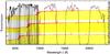 |
Fig. 1 ALHAMBRA filter transmission curve covering the optical to NIR. From top to bottom, the red curves show the typical redshifted spectrum of a star-forming galaxy at z ~ 1.5, z ~ 1.0 and z ~ 0.5. The gray shaded areas mark the position of the ALHAMBRA filters R8, I14, and z20, which highlights the position of the Balmer jump. To select the BJG samples, we use the filter directly redward of the gray filter to sample the end position of the Balmer jump. |
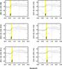 |
Fig. 2 Criteria for selecting star-forming galaxies. The solid and dashed lines show the color evolution of star-forming and passive galaxies, respectively. Red, green, and blue dashed lines show the passively evolving models with a formation redshift of zf = 2,3,6, respectively. Red, green, and blue solid lines show models that evolve with a constant star-formation rate for ages of 0.2, 1, and 2 Gyr. The horizontal dashed line indicates the color cut U2XnK ≡ (U2 − Xn) − (Xn − K) = 0. In each panel, the star-forming galaxies are located above this threshold. The yellow shaded regions mark the redshift range of the selected BJG samples in each color combination. Dashed vertical lines indicate the redshift 0.5 and 1.5. |
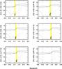 |
Fig. 3 Criteria for selecting star-forming galaxies. The solid and dashed lines show the color evolution of star-forming and passive galaxies, respectively. Red, green, and blue dashed lines show the passively evolving models with a formation redshift of zf = 2,3,6, respectively. Red, green, and blue solid lines show models that evolve with a constant star-formation rate for ages of 0.2, 1, and 2 Gyr. The horizontal dashed line indicates the color cut U2XnK ≡ (U2 − Xn) − (Xn − K) = 0. In each panel, the star-forming galaxies are located above this threshold. The yellow shaded regions mark the redshift range of the selected BJG samples in each color combination. Dashed vertical lines indicate the redshift 0.5 and 1.5. |
3.1. Selection of star-forming galaxies
We used the models of Bruzual & Charlot (2003) convolved with the ALHAMBRA filter system to define a two-color criterion to select star-forming galaxies analogously to the work of Daddi et al. (2004). They created the BzK color-selection technique to cull star-forming galaxies at z> 1.4. This technique is based on the Balmer jump, which is an indicator of recent star formation. They used the models of Bruzual & Charlot (2003) to identify the redshifted Balmer jump in the z-band, creating the color-selection criterion BzK ≡ (z − K)AB − (B − z)AB = −0.2; where BzK ≥ −0.2 selects star-forming galaxies at z> 1.4. Our approach is analogous to the BzK method in the sense that we also used the Bruzual & Charlot (2003) models, but we recorded redshifted Balmer jumps in various (diverse) medium bands to select galaxies at different redshifts. This situation is illustrated in Fig. 1, which shows the typical spectrum of a star-forming galaxy redshifted to z ~ 0.5, z ~ 1.0 and z ~ 1.5. The ALHAMBRA bands are overplotted from the optical to NIR ranges. We chose the U2-band to sample the region before the Balmer jump instead of the B-band. We selected the U2 band because it reaches a higher completeness level than U1. Objects that were not detected in the U2 band were also considered in our selection, and their magnitude limit was used. Redder bands might sample weak features blueward of the Balmer jump of low-redshift galaxies z< 0.4. The K band is exactly the same as was used by Daddi et al. (2004), while the z-band was replaced with the variable Xn-band, which covers the optical range from 613 Å to 954 Å. This means that Xn can be any ALHAMBRA filter from R9 to z20 (see Table 1). The Xn-band samples the region directly redward of the Balmer jump, hence the U2 − Xn color indicates the galaxy redshift range depending on the selected n. On the other hand, the Xn − K color registers the duration of the star formation age. The different panels in Figs. 2 and 3 show the theoretical evolution (Bruzual & Charlot 2003) of the U2XnK ≡ (Xn − K) − (U2 − Xn) color as a function of redshift with 9 <n< 20 (Xn = R9,....,z20). Red, green, and blue solid lines show the U2XnK-color evolution of constant star-formation rate models for ages 0.2, 1, and 2 Gyr and reddening E(B − V) = 0.3. Red, green, and blue dashed lines show the U2XnK-color evolution of passively evolving models for formation redshift of zf = 2,3 and 6. In each panel, the star-forming models always lie in the region U2XnK> 0. Consequently, to select a sample at redshift higher than z ~ 0.5, a combination that involves a Xn filter redder than R9 must be used, as we show in the bottom panels of Figs. 2 and 3.
3.2. BJG samples
We used the condition U2XnK ≡ (U2 − Xn) − (Xn − K) > 0 and the homogeneous coverage in the optical range of the ALHAMBRA filter system, where n ranges from 9 to 20 (Xn = R9,..,z20), to select galaxies at redshift z> 0.5, 0.6, 0.7, 0.8, 0.85, 0.95, 1.05, 1.1, 1.2, 1.25, and 1.3. In each ALHAMBRA filter set U2XnK, this color condition selects star-forming and passive galaxies in the wide redshift range. Theoretically, these selected passive galaxies always lie at higher redshift (i.e., Δz> 0.25) than the selected star-forming galaxies. To select galaxies in a narrow redshift range, we used more than one color condition; first the (U2 − Xn) − (Xn − K) > 0 condition with n = j, to select all galaxies above certain redshift zj , and second we subtracted the higher redshift samples, selected with n ≥ j + 1 (passive and star forming), from the first galaxy selection. For example, our lowest redshift sample was selected by imposing the condition U2R9K = 0 (i.e., select galaxies at z> 0.5) and subtracting the galaxy samples selected by U2XnK> 0 with n ≥ 10, which selects all galaxies at z> 0.6. In this way, only the star-forming galaxies in the redshift range 0.5 <z< 0.6 were selected (see yellow shaded region in Figs. 2 and 3). Following this method and using the homogeneous separation between each ALHAMBRA band, we selected eleven star-forming galaxy samples peaking at z ~ 0.55,0.65,0.75,0.8,0.9,1.0,1.05,1.15,1,2,1.25, and z ~ 1.4 by culling the galaxies that satisfied the star-forming criterion U2XnK ≡ (U2 − Xn) − (Xn − K) > 0, where Xn = R9,...,z19 and cleaned of higher redshift galaxies by subtracting the samples that satisfied U2XnK> 0, with n ≥ 10,...,20. Table 2 summarizes the properties of the selected samples using the method described above. We ensured that all samples are roughly independent of each other by removing the high-redshift samples that were selected using the Xn filters with n ≥ j + 1 (see Col. 3 of Table 2) from the sample selected with the filter Xn = j.
Properties of the BJG selected samples.
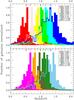 |
Fig. 4 Photometric redshift distribution of the selected samples. Upper panel: red, pink, yellow, light green, cyan, and blue histograms show the zBPZ distribution of the BJG1,BJG3,BJG5,BJG7,BJG9, and BJG11 samples, respectively. Lower panel: magenta, orange, dark green, green, and light blue histograms show the zBPZ distribution for the BJG2,BJG4,BJG6,BJG8, and BJG10 samples, respectively. The vertical colored lines show the median of the zBPZ distribution for the selected samples. The label locate in the upper-right corner reports the median redshift. |
4. Physical properties of the BJG samples
In this section, we characterize each BJG sample by providing a mean characteristic value of its redshift, absolute magnitude, stellar mass, age, star formation rate, etc.
Median physical properties of the BJG samples.
4.1. Photometric redshifts
We used the Bayesian photometric redshift (zBPZ) published in the Gold ALHAMBRA catalogs (Molino et al. 2014) to verify our selection method. The BPZ code was optimized to determine photometric redshifts, for details on the zBPZ calculations see Molino et al. (2014) and Benitez et al. (2009). Figure 4 shows the zBPZ distribution of the eleven BJG samples. To better visualize the distribution tails, the upper panel shows the BPZ distribution of the BJG1,BJG3,BJG5,BJG7,BJG9, and BJG11 samples, while the lower panel presents the BJG2,BJG4,BJG6,BJG8, and BJG10 samples. The median of zBPZ distribution, reported in Table 3, clearly agree with the median of the expected redshift range estimated through the two-color selection criteria reported in Table 2.
4.2. SED fitting
For each galaxy of the BJG samples, we fit the 20 optical bands plus the three NIR bands using the Bayesian SED modeling code iSEDfit (Moustakas et al. 2013). After we fixed the redshift to the best-fit value given by BPZ in the ALHAMBRA catalog (Molino et al. 2014), iSEDfit calculated the marginalized posterior probability distributions for the physical parameters in a certain model space that was previously defined. Using a Monte Carlo technique, we generated 20,000 model SEDs with delayed star formation histories SFH ~te− t/τ, where τ is the star formation timescale. The SEDs were computed employing the flexible stellar population synthesis models (FSPS, v 2.4; Conroy et al. 2009; Conroy & Gunn 2010) that are based on the miles (Sanchez-Blázquez et al. 2006) and Basel (Lejeune et al. 1997, 1998; Westera et al. 2002) stellar libraries. We assumed a Chabrier (2003) initial mass function from 0.1−100 M⊙ and the time-dependent attenuation curve of Charlot & Fall (2000). We adopted uniform priors on stellar metallicity Z/Z⊙ ∈ [ 0.04,1.0 ], galaxy age t ∈ [ 0.01,age(zBPZ) ] Gyr, rest-frame V-band attenuation AV ∈ [ 0−3 ] mag, and star formation timescale τ ∈ [ 0.01,age(zBPZ) ] Gyr, where age(zBPZ) is the age of the Universe at each galaxy’s photometric redshift.
Figures 9 and 10 show the SEDs of a galaxy randomly picked from each BJG sample. The green filled symbols show the data and their error bar. The model that minimize the χ2 is drawn with the red line. The universe of models, generated using the aforementioned setup, and scaled by their reduced χ2 is shown with the blue shading.
For each BJG sample and certain physical properties, the median value of the sum of the posterior probability distributions were calculated and are reported in Table 3. The uncertainties indicate the 1σ confidence level; to account for asymmetric distributions, we determined the percentiles 16 and 84.
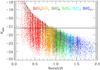 |
Fig. 5 Absolute magnitude as a function of redshift. The colored dots represent a galaxy of each BJG sample, using the same color code than in Fig. 4. The horizontal solid line shows the absolute magnitude cut Kabs = −21.2. |
4.3. Comparison between BJG samples
In this subsection, we compare the properties derived from SED fitting of the BJG samples for galaxies of similar K-band absolute magnitude, i.e. similar stellar mass. Therefore, in addition to restricting the BJG samples within the magnitude survey limit (see Sect. 3), we applied an absolute magnitude limit for all samples. In the following, we determine the most appropriate absolute magnitude limit that allows us to build these samples. Figure 5 shows the K-band absolute magnitude, obtained through the iSEDfit, as a function of BPZ redshift. The red, orange, green, cyan, light blue, and blue dots indicate the galaxies in the BJG1, BJG4, BJG6, BJG7, BJG9, and BJG11 samples with apparent magnitude brighter than the magnitude survey limit K = 22, respectively. We can note that partly as a result of the Malquist bias, the farthest sample BJG11 is roughly complete only until Kabs = −22.5 (blue dots). However, by choosing this bright absolute limit to compare all BJG samples, we restrict our study to the most massive and bright objects and also enormously reduce the statistics for each sample, especially at low redshift. Hence, we decided to study all objects brighter than Kabs = −21.2, which corresponds to the absolute limit where the BJG5 sample at z ~ 1 is complete and comparable, in terms of Kabs luminosity, to the other lower redshift BJGn< 6 samples. In Fig. 5 the black solid line shows the absolute magnitude limit Kabs = −21.2. We chose the z ~ 1 limit because the ALHAMBRA Gold data are an F814W (i.e., almost an I-band) selected catalog and thus are less sensitive to galaxies at z ≥ 1 with a pronounced Balmer jump. For galaxies at z ≥ 1, the spectral region directly blueward of the Balmer jump is barely or not at all detected in the F814W because the Balmer jump falls in the I13 band and the region directly blueward of it falls in the R12 band. Since the F814W image detection is a linear combination involving the R12 band, these types of galaxies are barely or not at all detected as sources in the final catalog. We expect a deeper selection of galaxies with a pronounced Balmer jump at z< 1. Hence, the BJG samples at  selected from Xn ≤ 13 bands are optimized to be complete according to the F814W selection, whereas the samples at z ≥ 1 are incomplete. The level of incompleteness of the BJGn ≥ 6 samples is difficult to quantify because there may be many effects working together (e.g., the F814W band is a linear combination of ALHAMBRA bands and blueward regions of the Balmer jump that are undetectable as a result of intrinsic galaxy properties such as redshift and dust excess). To minimize the incompleteness of our samples in the comparison of the physical properties at different redshifts, we redefine the first five BJG samples in the following by selecting all galaxies brighter than Kabs = −21.2. Furthermore, the BJGn samples with n ≥ 6 are not considered in the following analysis. Table 4 presents the properties of the final sample definition (BJGKn, with n< 6), which takes into account the absolute luminosity cut (Kabs = −21.2). In Fig. 6 the comparison of the physical properties of galaxies with similar K-band luminosity is shown. Red squares show the median value of the probability distribution for each BJGKn sample (with n< 6), while the colored areas indicate their dispersion. The error bars show the median error of the properties derived through the iSEDfit. In Sect. 6.3 these results are discussed.
Median physical properties of the BJGK samples considering the absolute magnitude limit K = −21.2.
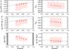 |
Fig. 6 Evolution of the physical properties of the BJGKn< 6 samples. The panels show the median of the probability distribution of (top to bottom and left to right) the specific star formation rate, star formation rate, age, B-band luminosity, K-band luminosity, and stellar mass. Red squares show the evolution of BJGKn< 6 galaxies brighter than K = −21.2. The colored areas represent the dispersion of each sample. The error bars correspond to the median error of the physical properties determined by the iSEDfit. Dashed lines show the fit to the CANDELS analysis taken from van Dokkum et al. (2013) for galaxies of stellar masses similar to the Milky Way. |
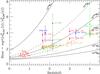 |
Fig. 7 Evolution of the bias factor, calculated with the variance at 8 h-1 Mpc, for samples of star-forming galaxies. Red diamonds indicate the BJGKn< 6 samples. At z ~ 2, the gray, blue, red, green, and light green squares show the sBzK samples of Hayashi et al. (2007), Blanc et al. (2008), Hartley et al. (2008), Lin et al. (2012), and McCracken et al. (2010), respectively. Yellow squares show the BMandBX selected galaxies of Adelberger et al. (2005). At z ~ 3, the blue, green, and red squares indicate the LBGs selected by Yoshida et al. (2008), Kashikawa et al. (2006), Hildebrandt et al. (2007), Ouchi et al. (2005), respectively. Gray squares show the Ly-α emitters selected by Guaita et al. (2010), Gawiser et al. (2007). The lines show the bias evolution for different halo masses (Sheth et al. 2001), which are indicated below each line at the right side of the panel. |
5. Halo masses through clustering analysis
In hierarchical clustering, structures build up in time from small density fluctuations. Small structures agglomerate to build large structures. Dark matter halos are biased tracers of the underlying matter density field. Massive halos lie in higher and rarer density peaks and are more clustered than lower mass halos. If a galaxy population is hosted by halos of a given mass, then the clustering amplitude of the galaxy population, compared to the expected dark matter clustering at the same redshift, can be used to derive the typical halo mass corresponding to that galaxy population. This is encapsulated in the bias parameter, b, defined as b2 = ξgal(r) /ξDM(r), where ξgal and ξDM are the two-point spatial correlation functions for galaxies and dark matter, respectively. The correlation function at a certain redshift, ξ(r,z), can be characterized with a power law and a correlation length, r0, through ξ(r,z) = (r/r0(z))γ, where γ is the power index. For sparse samples and at small scales this representation is typically used. In larger surveys and simulations the correlation function is usually modeled by combining terms for galaxies in the same halo and in different ones (Zehavi et al. 2011; Contreras et al. 2013).
In the following, we measure the bias and masses of the halos that host the BJGKn< 6 samples. Specifically, for each BJGKn< 6 sample, we calculate the two-point angular correlation function, and then, using the Limbers deprojection, given a redshift distribution and a cosmological model, we calculate the correlation length. The bias parameter follows from r0 through  , where σ8,gal (σ8,DM) is the root mean square fluctuation amplitude in 8 h-1 Mpc spheres of galaxies (dark matter). The halo mass is obtained from the bias by using the models of Sheth et al. (2001). We chose this procedure and the 8 h-1 Mpc scale to directly compare our results with previous works that connected progenitors and descendants of samples of star-forming galaxies (see Fig. 7, Adelberger et al. 2005; Ouchi et al. 2005; Kashikawa et al. 2006; Gawiser et al. 2007; Hildebrandt et al. 2007; Hayashi et al. 2007; Blanc et al. 2008; Hartley et al. 2008; Yoshida et al. 2008; Guaita et al. 2010; McCracken et al. 2010; Lin et al. 2012). More detailed treatments, such as considering both halo terms and different scales, are beyond the scope of this paper.
Clustering properties of the BJGK samples.
5.1. Angular correlation and correlation length
To determine the angular correlation function, we used the Landy and Szalay (1993) prescription  (1)where Ngg and Nrr are the number of pairs at a separation θ of galaxies in the catalog and points in a random catalog with the same layout as the galaxy sample, respectively. Ngr is the cross number of points between the galaxy and random distributions. For our calculations we considered five ALHAMBRA fields (see Sect. 2) that encompass 36 pointing catalogs. Errors were estimated by a jackknife method, which has been shown to be a robust error estimator (Zehavi et al. 2011; Cabré et al. 2007), although it can overestimate the variance on small scales (Norberg et al. 2009). We calculated the angular correlation function 36 times, each time eliminating one catalog out of the 36 available. The uncertainty was estimated as the variance of w(θ). We followed the method of Infante (1994), Quadri et al. (2007) to correct for the integral constraint. As mentioned above, to calculate r0 we used the power-law approximation ξ(r,z) = (r(z) /r0(z))− γ that depends on the spatial separation and redshift. Likewise, the two-point angular function is w(θ,z) = Aw(z)θ(1 − γ), where Aw(z) is the angular amplitude. By fitting the correlation function to this power law, between 0.005 and 0.2 degree, the Aw(z) is inferred. The angular amplitudes are reported in Table 5. To calculate the spatial from the angular function, we used the Limber (1953) inversion, which requires a redshift distribution N(z), and assumed a cosmological model. Limber’s inversion involves solving the following integral (Kovac et al. 2007):
 ![Mathematical equation: \begin{equation} r_0^\gamma=\frac{ A_w (c/H_0) {[\int {N(z) {\rm d}z}]}^2}{C_\gamma \int{F(z) D_\theta^{1-\gamma}(z) N^2(z) g_d(z) {\rm d}z} } , \end{equation}](/articles/aa/full_html/2016/04/aa27552-15/aa27552-15-eq303.png) (2)where the cosmology plays a role in the Hubble parameter H0,
(2)where the cosmology plays a role in the Hubble parameter H0, ![Mathematical equation: \hbox{$g_d(z)= (1+z)^2\sqrt{1+\Omega_{\rm m} z+\Omega_\Lambda[(1+z)^{-2}-1]}$}](/articles/aa/full_html/2016/04/aa27552-15/aa27552-15-eq305.png) , and in the angular diameter distance Dθ. The parameter Cγ depends on the power index such that
, and in the angular diameter distance Dθ. The parameter Cγ depends on the power index such that ![Mathematical equation: \hbox{$C_\gamma=\Gamma(0.5)\frac{\Gamma[0.5(\gamma-1)]}{\Gamma[0.5\gamma]}$}](/articles/aa/full_html/2016/04/aa27552-15/aa27552-15-eq308.png) . To be consistent internally and compare our results with other works (Adelberger et al. 2005; Ouchi et al. 2005; Kashikawa et al. 2006; Hayashi et al. 2007; Hildebrandt et al. 2007; Gawiser et al. 2007; Blanc et al. 2008; Hartley et al. 2008; Yoshida et al. 2008; Guaita et al. 2010; McCracken et al. 2010; Lin et al. 2012), the value of γ was fixed to the canonical γ = 1.8. This value is fully justified by experiments where γ was left free and is consistent with the clustering of luminosity-selected ALHAMBRA samples (Arnalte-Mur et al. 2014). F(z) accounts for the redshift evolution of the correlation function, where F(z) = (1 + z)− (3 + ϵ), and we used ϵ = −1.2, which corresponds to the value adopted for a constant clustering in comoving coordinates (Quadri et al. 2007). To calculate the correlation length error, we took the error contribution from the amplitude of the angular correlation function, the Poissonian errors (~
. To be consistent internally and compare our results with other works (Adelberger et al. 2005; Ouchi et al. 2005; Kashikawa et al. 2006; Hayashi et al. 2007; Hildebrandt et al. 2007; Gawiser et al. 2007; Blanc et al. 2008; Hartley et al. 2008; Yoshida et al. 2008; Guaita et al. 2010; McCracken et al. 2010; Lin et al. 2012), the value of γ was fixed to the canonical γ = 1.8. This value is fully justified by experiments where γ was left free and is consistent with the clustering of luminosity-selected ALHAMBRA samples (Arnalte-Mur et al. 2014). F(z) accounts for the redshift evolution of the correlation function, where F(z) = (1 + z)− (3 + ϵ), and we used ϵ = −1.2, which corresponds to the value adopted for a constant clustering in comoving coordinates (Quadri et al. 2007). To calculate the correlation length error, we took the error contribution from the amplitude of the angular correlation function, the Poissonian errors (~ ), and the effects of the photometric redshift error in shifting and broadening N(z) into account.
5.2. Bias and mass measurements
In turn we estimated the bias parameter, b, from the correlation length. As pointed out above, b is related to r0 through the spatial correlation function by b2 ≈ ξgal(r,z) /ξDM(r,z) or  . The numerator
  was taken from Peebles (1980) (Eq. (59.3)), where J2 is a parameter defined in terms of γ as J2 = 72/ [ (3−γ)(4 − γ)(6 − γ)2γ ]. We fixed the spatial scale at 8 h-1 Mpc such that ξgal(8,z) = (r0(z)/8 h-1Mpc)γ. The evolution of the dark matter density variance in a comoving sphere of radius 8 h-1 Mpc is
  , where D(z) is the linear growth factor at redshift z. The bias measured for each BJGK sample at a scale of 8 h-1 Mpc is reported in Table 5.
Figure 7 shows the bias factor as a function of redshift for the BJGK samples (red diamonds). The lines show the bias evolution for different halo masses (Sheth et al. 2001), which are indicated below each line at the right side of the panel. The BJGK samples approximately follows the bias evolution of halos of masses ~1012.5 h-1 M⊙. Finally, we calculated the halo mass using Eq. (8) of Sheth et al. (2001), which relates the bias with the peak height, ν = δsc(z) /σ(M,z), where δsc is the critical overdensity computed using the spherical collapse model. Here we assumed δsc = 1.69. Then, the halo mass Mh was obtained through σ(M,z) evaluated at the redshifts of the BJGK samples listed in Table 4. In Fig. 8 the halo mass of the BJGK samples as a function of redshift is shown. This is calculated with the variance at 8 h-1 Mpc. Squares show the median values of the halo mass, while polygons show a conservative limit. This draws the mass limits considering the 1σ deviation of the redshift and bias. The results are presented in Table 5.
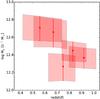 |
Fig. 8 Halo mass as function of redshift for the BJGKn< 6 samples. Squares show the median values of the halo mass, while polygons draw the mass limit taking into account the error of redshift and bias. |
6. Discussion
6.1. Selection technique
The new two-color selection technique U2XnK based on ALHAMBRA medium-bands allows us to extract eleven samples of star-forming galaxies at z> 0.5 in narrower redshift ranges than was possible in previous studies (Daddi et al. 2004; Steidel et al. 2004; Adelberger et al. 2005). This selection method is based purely on the ALHAMBRA photometric data and does not depend on the models assumptions, method, or templates used to determine the photometric redshifts or properties derived from SED fit. We validated this technique with the Bruzual & Charlot (2003) models and also checked other stellar population synthesis models, which give consistent results.
The ALHAMBRA GOLD data are an F814W-selected catalog, thus it is less sensitive to the regions blueward of the Balmer jump of galaxies at z> 1. The R12 band only contributes to 10% of the final F814W detection image, while the I13, and I14 bands contribute 18% each. Hence, the detection in the F814W image becomes poorer for galaxies at z ≥ 1 with a pronounced Balmer jump.
To avoid contamination of low-redshift galaxies in our samples, we used the bluest band available to sample the region blueward of the Balmer jump. Hence, we studied the detection level of the U1 and U2 , which reaches 97% and 99.7%, respectively. Since U2 has a higher detection level than U1, we tailored the selection technique using the U2 band.
To select samples at z< 0.5, we tried to use filters bluer than the R9, whose central wavelength is lower than 613.5 Å. Nevertheless, the theoretical evolution of the color U2Xn< 9K of passive and star-forming galaxies, based on the Bruzual & Charlot (2003) models, tends to occupy the same locus in the color-redshift (U2Xn< 9K − z) plane. Hence, it does not allow separating the star-forming from the passive galaxies as clearly as for the U2XnK selection with n> 9 (see Figs. 2 and 3).
The number density of each BJG sample decreases with redshift, probably because of the nature of these objects or because of the Malquist-bias selection effect in the U2-band, which we did not consider here. In addition, we verified our selection method with the BPZ photometric redshifts, whose uncertainty increases with redshift, and therefore the number densities might be underestimated according to δz(BPZ) = 0.014 z(BPZ).
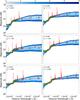 |
Fig. 9 Spectral energy distribution of a star-forming galaxy in the ALHAMBRA survey. From left to right and top to bottom, the panel shows the SED of a galaxy randomly picked from the BJG1, BJG2, BJG3, BJG4, BJG5, and BJG6 samples. The filled green dots show the ALHAMBRA photometric data. The red line shows the model that minimizes the χ2 found by iSEDfit, the minimum reduced χ2 is indicated in the upper left corner, in addition to the BPZ photometric redshift. The black squares mark the ALHAMBRA photometry of the best model. The blue shading shows the universe of models, generated by iSEDfit (see Sect. 4.2), scaled by their reduced χ2. The color bar indicates the reduced χ2 scale. |
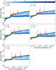 |
Fig. 10 Spectral energy distribution of a star-forming galaxy in the ALHAMBRA survey. From left to right and top to bottom, the panel shows the SED of a galaxy randomly picked from the BJG7, BJG8, BJG9, BJG10, and BJG11 samples. The filled green dots show the ALHAMBRA photometric data. The red line shows the model that minimizes the χ2 found by iSEDfit, the minimum reduced χ2 is indicated in the upper left corner, in addition to the BPZ photometric redshift. The black squares mark the ALHAMBRA photometry of the best model. The blue shading shows the universe of models, generated by iSEDfit (see Sect. 4.2), scaled by their reduced χ2. The color bar indicates the reduced χ2 scale. |
Based on this color technique (visual inspection of Figs. 2 and 3), the redshift distributions should be narrower than in Fig. 4. The distributions can become wider if the errors of the photometric redshifts are properly taken into account. The mean formal BPZ errors of the BJG1 and BJG11 samples are 0.02 and 0.03, which corresponds to 20% and 30% of the total expected width (≤0.1), respectively. We performed simulations considering Gaussian redshift distributions filled randomly using the same number of galaxies found in each sample, the expected width (0.1), and the formal BPZ error δz(BPZ) = 0.014(1 + z(BPZ)). By perturbing the photometric redshift with its corresponding error and randomly choosing a positive or negative variance, the width of the distributions increases by a factor of 1.5 for the first BJG1 sample and up to twice this value for the BJG11 sample with increasing redshift. Clearly, higher photometric redshift errors increase the distribution width. In the AHAMBRA data, BPZ tends to lower precision at I< 24.5 AB (Molino et al. 2014). The global redshift distribution shows a mean of ⟨ z ⟩ = 0.86 at this magnitude limit. Hence the distributions at z ≥ 0.9 tend to broaden even more because the photometric redshift errors exceed 0.014(1 + z). For a distribution at z ~ 1 with an original width of 0.1 and δz(BPZ) = 0.03(1 + z(BPZ)), the width increases up to three times. Outliers that are due to either photometric redshift or the color selection technique can also contribute to the tails and may also broaden the photometric redshift distributions.
We also investigated the selection method by creating an Xn band composed of two, three, and four consecutive ALHAMBRA bands. This increased the statistics, accuracy, and width of the redshift distribution of each sample. Nevertheless, to fully exploit the capabilities of a multi-medium band survey in selecting galaxies in small redshift ranges, we chose to use a unique band in our selection method.
Viironen et al. (2015) have shown that is possible to obtain a clean galaxy sample using the redshift probability distributions, which is by definition (intrinsically) not complete. The fact of choosing a certain probability threshold implies that some galaxies will not be considered in the final sample. To overcome the problem of purity versus completeness, they suggested using the information of the whole zPDF to select each sample. In this work we tailored and used a two-color criterion that considered all the observational data available, selecting a complete sample, but at the same time was probably more contaminated than the samples selected according to redshift probability distributions. We used the zBPZ-BJG distributions to calculate this contamination by estimating how many objects have a BPZ redshift lower or higher than 3σ of its corresponding redshift distribution. Thus, it encompasses from 1% to 15% of each sample depending on redshift. Specifically, 1%, 2%, 2%, 3%, 4%, 5%, 6%, 7%, 8%, 10%, 12%, and 15% of the sample BJG1, BJG2, BJG3, BJG4, BJG5, BJG6, BJG7, BJG8, BJG9, BJG10, and BJG11, respectively.
6.2. Progenitors and descendants
We obtained the halo masses where our BJGK samples reside (see Fig. 8). The galaxy samples of similar K-band absolute magnitude reside in halos of 1012.5 ± 0.2 M⊙. In terms of progenitors and descendants for the median halo mass, the progenitors are the LBGs with R< 25 at z ~ 3 (Adelberger et al. 2005; Hildebrandt et al. 2007), the sBzK galaxies with K ≤ 23 at z ~ 2 (Hayashi et al. 2007; Hartley et al. 2008; McCracken et al. 2010; Lin et al. 2012) and the descendants in the local Universe are galaxies with luminosities around 2 L∗ (see Fig. 7). For halos around the upper limit 1012.7 M⊙, we found as progenitors at z ~ 3 the LBGs (Hildebrandt et al. 2007) with R ≤ 24 and at z ~ 2 the sBzK galaxies with K ≤ 23 (Hartley et al. 2008; Lin et al. 2012). The descendants are galaxies with luminosities around 3 L∗. For the halos around the lower limit 1012.3 M⊙, the progenitors are the LBGs at z ~ 4 (Kashikawa et al. 2006; Ouchi et al. 2005) with I or z ≤ 27, the LAE galaxies at z ~ 3 (Gawiser et al. 2007), and the sBzK galaxies (Hayashi et al. 2007) with K< 23 at z ~ 2. The descendants are galaxies with luminosities around 1 L∗. The increment of the median halo mass of ~0.4 dex, between z = 1.0 and z = 0.5, follows the observed mass increment in numerical simulations (Millennium, Fakhouri et al. 2010). This suggests that we trace the evolution of halos with masses of around ~1012.5 from z = 1.0 to z = 0.5, and hence the evolution of the physical properties, as is shown in Fig. 6. So far, we argued based on clustering measurements that our five sets of galaxies BJGKn< 6 represent a coeval and homogeneous population of star-forming galaxies.
The bias and hence halo mass of the BJGK samples is higher on average than those found in Hurtado et al. (2016) for star-forming galaxies. For all redshift ranges studied, our correlation lengths are 20% higher than in their work, suggesting that we selected more massive galaxies. This might be due to the different galaxy selection methods and to the absolute magnitude thresholds used to define complete samples. Nevertheless, the main difference is caused by the method and the scale that we chose to calculate the bias and hence the halo mass. Hurtado et al. (2016) calculated the bias for the scale range 1.0 <r< 10 Mpc, while in this work we evaluated the bias on the scale 8 h-1 Mpc to compare our results with previous works that also studied the progenitors and descendants of star-forming galaxies. By taking this approach, we obtained halo masses 0.7 dex higher than in (Hurtado et al. 2016).
6.3. Physical properties
We performed an accurate estimation of the physical properties derived from SED fitting (e.g., absolute magnitude, stellar mass, and star formation rate) and characterized each sample as a whole with the median of each of these properties. Figure 6 shows the median of the probability distribution of stellar mass, absolute magnitude, and star formation rate for the BJGKn< 6 (red squares) samples as a function of redshift. In the stellar mass panel, the dashed line shows the evolution of the stellar mass for galaxies with present-day stellar masses of log (M∗) ≈ 10.7, such as our Milky Way galaxy. The data are taken from the analysis of the CANDELS survey by van Dokkum et al. (2013). The observed mass growth determined by van Dokkum et al. (2013), which slightly increase by a factor of 0.1 dex from z = 1 to z = 0.5, agrees well with the flat behavior found in this work. In the star formation rate panel, the dashed line shows the evolution of the implied star formation rate that is caused by the evolution of the stellar mass of galaxies with present-day stellar masses of log (M∗) ≈ 10.7, such as our Milky Way, also taken from van Dokkum et al. (2013). Our results are slightly lower, suggesting that the SFR is sufficient to account for the increment in stellar mass between z = 1 and z = 0.5 and that major mergers play a minor role in this redshift range. The evolution of the SFR and sSFR resembles the expected main-sequence behavior of star-forming galaxies (Rodighiero et al. 2011). The BJGK evolution from z ~ 1 to z = 0 of the B-band absolute luminosity agrees with the evolution measured by Tasca et al. (2014). They found that the contribution of disks to the total B-band luminosity decreases by 30% from z ~ 1 to z = 0, while for the BJGs the median B-band luminosity decreases by a factor of 0.5 dex. The distribution of galaxy ages obtained by iSEDfit has a large dispersion, but even so, its increment between two epochs corresponds to the Universe age increment indicated by the redshift. According to the models of Lagos et al. (2014), galaxies of properties similar to the BJGs host most of the neutral gas at 0.5 <z< 1.5. Hence the BJG samples contain tentative targets to sample the neutral gas with submillimeter surveys.
7. Conclusions
We have selected eleven samples of star-forming galaxies by using a two-color technique based on the Bruzual & Charlot (2003) models convolved with the ALHAMBRA filters. Using clustering arguments, we confirmed that five out of the eleven sets of galaxies, that is, the BJGKn< 6, represent a coeval and homogeneous population of star-forming galaxies. The properties derived from SED fitting, such as stellar mass, star formation rate, age, and absolute luminosity of each BJGKn< 6 sample were characterized as a whole, allowing us to study their putative evolution as a function of redshift. The main results are summarized below.
We tailored a two-color selection technique, based on the Bruzual & Charlot (2003) models and the Balmer jump, that selects star-forming galaxies in the redshift range 0.5 <z< 1.5. We selected eleven samples composed of Balmer-jump Galaxies, dubbed BJG. The number of photometric-redshift outliers in these color-selected samples increases with redshift, ranging from 1% to 15%.
We created a subsample of BJG, dubbed BJGKn with n< 6, which considered only the BJGn< 6 galaxies brighter than Kabs ~ −21.2. The stellar mass of the BJGK samples changes almost not at all with redshift,suggesting that major mergers played a minor role in the evolution of the BJGK galaxies. The SFR evolution accounts for the small variations of the stellar mass, from z ~ 1 to z ~ 0.5, suggesting that star formation and minor mergers are the main channels of mass assembly. Although the distribution of galaxy ages obtained by iSEDfit has a large dispersion, the evolution of the galaxy age agrees with the evolution of the Universe age.
The BJGKn< 6 samples reside in halos of 1012.5 ± 0.2 M⊙, whose progenitors are the LBGs with R ≤ 24 at z ~ 3 (Hildebrandt et al. 2007) and the sBzK galaxies (Lin et al. 2012; Hartley et al. 2008; McCracken et al. 2010) with K ≤ 23 at z ~ 2. The descendants in the local Universe are galaxies with luminosities around 1–3 L∗ (for details see Fig. 7).
The similar increment of the median halo mass between z = 1.0 and z = 0.5 of our observational results and numerical simulations (Millennium, Fakhouri et al. 2010) suggests that we trace the evolution of halos of masses around ~1012.5 from z = 1.0 to z = 0.5, and hence the putative evolution of the physical properties of the galaxies hosted by these halos (see Fig. 6).
The homogeneous coverage of the ALHAMBRA optical bands from R9 to z20 allows us to trace the evolution of the baryonic processes occurring on star-forming galaxies from z ~ 1.0 to z ~ 0.5, which reside in halos of masses ~1012.5 h-1 M⊙. This roughly corresponds to a stellar mass upper (lower) limit of ~1011 M⊙(1010 M⊙). Deeper ALHAMBRA data and near-infrared selected catalogs would allow us to study the evolution of the physical properties in halos of masses lower than 1012.5 M⊙ from z ~ 0.5 to z ~ 1.5.
Acknowledgments
The work presented in this paper is based on observations taken at the Centro Astronómico Hispano Alemán (CAHA) at Calar Alto, operated jointly by the Max-Planck-Institut für Astronomie and the Instituto de Astrofísica de Andalucía (IAA–CSIC). P.T. and A.M.A. acknowledge support from FONDECYT 3140542 and FONDECYT 3160776, respectively. L.I., A.M.A., P.T., S.G., N.P. acknowledge support from Basal-CATA PFB-06/2007. E.J.A. acknowledges support from the Spanish Ministry for Economy and Competitiveness and FEDER funds through grant AYA2013-40611-P. A.F.S., V.J.M. and P.A.M. acknowledge partial financial support from the Spanish Ministry for Economy and Competitiveness and FEDER funds through grant AYA2013-48623-C2-2, and from Generalitat Valenciana through project PrometeoII 2014/060. B.A. acknowledges received funding from the European Union’s Horizon 2020 research and innovation programme under the Marie Sklodowska-Curie grant agreement No. 656354.
References
- Arnalte-Mur, P., Martínez, V. J., Norberg, P., et al. 2014, MNRAS, 441, 1783 [NASA ADS] [CrossRef] [Google Scholar]
- Adelberger, K., Steidel, C. C., Pettini, M., et al. 2005, ApJ, 619, 697 [NASA ADS] [CrossRef] [Google Scholar]
- Aparicio Villegas, T., Alfaro, E. J., Cabrera-Caño, J., et al. 2010, AJ, 139, 1242 [NASA ADS] [CrossRef] [Google Scholar]
- Benitez, N., Moles, M., Aguerri, J. A. L., et al. 2009, ApJ, 692, L5 [NASA ADS] [CrossRef] [Google Scholar]
- Blanc, G., Lira, P., Barrientos, L. F., et al. 2008, ApJ, 681, 1099 [NASA ADS] [CrossRef] [Google Scholar]
- Bruzual, G., & Charlot, S. 2003, MNRAS, 344, 1000 [NASA ADS] [CrossRef] [Google Scholar]
- Bouwens, R. 2014, ApJ, 795, 126 [NASA ADS] [CrossRef] [Google Scholar]
- Bouwens, R. 2015, ApJ, 803, 34 [NASA ADS] [CrossRef] [Google Scholar]
- Cabré, A., Fosalba, P., Gaztañaga, E., & Manera, M. 2007, MNRAS, 381, 1347 [NASA ADS] [CrossRef] [Google Scholar]
- Chabrier, G. 2003, PASP, 115, 763 [NASA ADS] [CrossRef] [Google Scholar]
- Campbell, D. J. R., Baugh, C. M., Mitchell, P. D., et al. 2015, MNRAS, 452, 852 [NASA ADS] [CrossRef] [Google Scholar]
- Charlot, S., & Fall, S. M. 2000, ApJ, 539, 718 [NASA ADS] [CrossRef] [Google Scholar]
- Conroy, C., & Gunn, J. E. 2010, ApJ, 712, 833 [NASA ADS] [CrossRef] [Google Scholar]
- Conroy, C., Gunn, J. E., & White, M. 2009, ApJ, 699, 486 [NASA ADS] [CrossRef] [Google Scholar]
- Contreras, S., Baugh, C. M., Norberg, P., & Padilla, N. 2013, MNRAS, 432, 2717 [NASA ADS] [CrossRef] [Google Scholar]
- Cristóbal-Hornillos, D., Aguerri, J. A. L., Moles, M., et al. 2009, ApJ, 696, 1554 [NASA ADS] [CrossRef] [Google Scholar]
- Daddi, E., Cimatti, A., Renzini, A., et al. 2004, ApJ, 617, 746 [NASA ADS] [CrossRef] [Google Scholar]
- Daddi, E., Elbaz, D., Walter, F., et al. 2010, ApJ, 714, L118 [Google Scholar]
- Davé, R., Finlator, K., Oppenheimer, B. D., et al. 2010, MNRAS, 416, 1354 [Google Scholar]
- Dey, A., Soifer, B. T., Desai, V., et al. 2008, AJ, 677, 943 [Google Scholar]
- Elbaz, D., Dickinson, M., Hwang, H. S., et al. 2011, A&A, 533, A119 [NASA ADS] [CrossRef] [EDP Sciences] [Google Scholar]
- Fakhouri, O., Ma, C., & Boylan-Kolchin, M. 2010, MNRAS, 406, 2267 [NASA ADS] [CrossRef] [Google Scholar]
- Finoguenov, A., Guzzo, L., Hasinger, G., et al. 2007, ApJS, 172, 182 [Google Scholar]
- Gawiser, Francke, H., Lai, K., et al. 2007, ApJ, 671, 278 [NASA ADS] [CrossRef] [Google Scholar]
- Guaita, L., Gawiser, E., Padilla, N., et al. 2010, ApJ, 714, 255 [NASA ADS] [CrossRef] [Google Scholar]
- Guzzo, L., Cassata, P., Finoguenov, A., et al. 2007, ApJS, 172, 254 [NASA ADS] [CrossRef] [Google Scholar]
- Hayashi, M., Shimasaku, K., Motohara, K., et al. 2007, AJ, 660, 72 [CrossRef] [Google Scholar]
- Hartley, W. G., Lane, K. P., Almaini, O., et al. 2008, MNRAS, 391, 1301 [NASA ADS] [CrossRef] [Google Scholar]
- Hildebrandt, H., Pielorz, J., Erben, T., et al. 2007, A&A, 462, 865 [NASA ADS] [CrossRef] [EDP Sciences] [Google Scholar]
- Hurtado-Gil, L. L., Arnalte-Mur, P., Martínez, V. J., et al. 2016, ApJ, 818, 174 [NASA ADS] [CrossRef] [Google Scholar]
- Infante, L. 1994, A&A, 282, 353 [NASA ADS] [Google Scholar]
- Infante, L., Zheng, W., Laporte, N., et al. 2015, ApJ, 815, 18 [NASA ADS] [CrossRef] [Google Scholar]
- Kashikawa, N., Yoshida, M., Shimasaku, K., et al. 2006, AJ, 637, 631 [Google Scholar]
- Kovac, K., Somerville, R. S., Rhoads, J. E., Malhotra, S., & Wang, J. 2007, ApJ, 668, 15 [NASA ADS] [CrossRef] [Google Scholar]
- Lagos, C. P., Baugh, C. M., Zwaan, M. A., et al. 2014, MNRAS, 440, 920 [NASA ADS] [CrossRef] [Google Scholar]
- Lejeune, T., Cuisinier, F., & Buser, R. 1997, A&AS, 125, 229 [NASA ADS] [CrossRef] [EDP Sciences] [Google Scholar]
- Lejeune, T., Cuisinier, F., & Buser, R. 1998, A&AS, 130, 65 [NASA ADS] [CrossRef] [EDP Sciences] [Google Scholar]
- Lilly, S., Carollo, C. M., Pipino, A., Renzini, A., & Peng, Y. 2013, ApJ, 772, 119 [NASA ADS] [CrossRef] [Google Scholar]
- Lin, L., et al. 2012, AJ, 756 [Google Scholar]
- Madau, P., & Dickinson, M. 2014, ARA&A, 52, 415 [NASA ADS] [CrossRef] [Google Scholar]
- Mannucci, F., Cresci, G., Maiolino, R., Marconi, A., & Gnerucci, A. 2010, MNRAS, 408, 2115 [NASA ADS] [CrossRef] [Google Scholar]
- McCracken, H. J., Capak, P., Salvato, M., et al. 2010, AJ, 708, 202 [NASA ADS] [CrossRef] [Google Scholar]
- Moles, M., Benítez, N., Aguerri, J. A. L., et al. 2008, AJ, 136, 1325 [Google Scholar]
- Molino, A., Benitez, N., Moles, M., et al. 2013, MNRAS, 441, 2891 [Google Scholar]
- Moustakas, J., Coil, A. L., Aird, J., et al. 2013, AJ, 767, 50 [NASA ADS] [CrossRef] [Google Scholar]
- Norberg, P., Baugh, C. M., Gaztañaga, E., & Croton, D. J. 2009, MNRAS, 396, 19 [NASA ADS] [CrossRef] [Google Scholar]
- Norberg, P., Gaztañaga, E., Baugh, C. M., & Croton, D. J. 2011, MNRAS, 418, 2435 [NASA ADS] [CrossRef] [Google Scholar]
- Ouchi, M., Hamana, T., Shimasaku, K., et al. 2005, AJ, 635, L117 [Google Scholar]
- Padilla, N., Christlein, D., Gawiser, E., Marchesini, D., et al. 2011, A&A, 531, A142 [NASA ADS] [CrossRef] [EDP Sciences] [Google Scholar]
- Padilla, N., Salazar-Albornoz, S., Contreras, S., Cora, S. A., & Ruiz, A. N. 2014, MNRAS, 443, 2801 [Google Scholar]
- Peebles, P. J. E. 1980, The large scale structure of the Universe (Princeton: Princeton University Press), 435 [Google Scholar]
- Quadri, R., van Dokkum, P., Gawiser, E., et al. 2007, AJ, 654, 138 [Google Scholar]
- Rodighiero, G., Daddi, E., Baronchelli, I., et al. 2011, AJ, 739, L40 [NASA ADS] [CrossRef] [Google Scholar]
- Sanchez, S., Rosales-Ortega, F. F., Iglesias-Páramo, J., et al. 2014, A&A, 563, A49 [NASA ADS] [CrossRef] [EDP Sciences] [Google Scholar]
- Sanchez-Blázquez, P., Peletier, R. F., Jiménez-Vicente, J., et al. 2006, MNRAS, 371, 703 [NASA ADS] [CrossRef] [Google Scholar]
- Scoville, N., Aussel, H., Benson, A., et al. 2007, ApJS, 172, 150 [Google Scholar]
- Sheth, R. K., Mo, H. J., & Tormen, G. 2001, MNRAS, 323, 1 [NASA ADS] [CrossRef] [Google Scholar]
- Steidel, C., Giavalisco, M., Pettini, M., Dickinson, M., & Adelberger, K. L. 1996, ApJ, 462, L17 [NASA ADS] [CrossRef] [Google Scholar]
- Steidel, C., Shapley, A. E., Pettini, M., et al. 2004, ApJ, 604, 534 [NASA ADS] [CrossRef] [Google Scholar]
- Tasca, L. A. M., Tresse, L., Le Fèvre, O., et al. 2014, A&A, 564, L12 [NASA ADS] [CrossRef] [EDP Sciences] [Google Scholar]
- Tomczak, A., Quadri, R. F., Tran, K.-V. H., et al. 2014, AJ, 783, 85 [NASA ADS] [CrossRef] [Google Scholar]
- Troncoso, P., Maiolino, R., Sommariva, V., et al. 2014, A&A, 563, A58 [NASA ADS] [CrossRef] [EDP Sciences] [Google Scholar]
- van Dokkum, P., Leja, J., Nelson, E. J., et al. 2013, AJ, 771, L35 [CrossRef] [Google Scholar]
- Viironen, K., Marín-Franch, A., López-Sanjuan, C., et al. 2015, A&A, 576, A25 [NASA ADS] [CrossRef] [EDP Sciences] [Google Scholar]
- Westera, P., Lejeune, T., Buser, R., Cuisinier, F., & Bruzual, G. 2002, A&A, 381, 524 [NASA ADS] [CrossRef] [EDP Sciences] [Google Scholar]
- Yoshida, M., Shimasaku, K., Ouchi, M., et al. 2008, AJ, 679, 269 [CrossRef] [Google Scholar]
- Zehavi, I., Blanton, M. R., Frieman, J. A., et al. 2002, ApJ, 571, 172 [NASA ADS] [CrossRef] [Google Scholar]
- Zehavi, I., Zheng, Z., Weinberg, D. H., et al. 2011, AJ, 736, 59 [CrossRef] [Google Scholar]
All Tables
Median physical properties of the BJGK samples considering the absolute magnitude limit K = −21.2.
All Figures
|
Fig. 1 ALHAMBRA filter transmission curve covering the optical to NIR. From top to bottom, the red curves show the typical redshifted spectrum of a star-forming galaxy at z ~ 1.5, z ~ 1.0 and z ~ 0.5. The gray shaded areas mark the position of the ALHAMBRA filters R8, I14, and z20, which highlights the position of the Balmer jump. To select the BJG samples, we use the filter directly redward of the gray filter to sample the end position of the Balmer jump. |
| In the text | |
|
Fig. 2 Criteria for selecting star-forming galaxies. The solid and dashed lines show the color evolution of star-forming and passive galaxies, respectively. Red, green, and blue dashed lines show the passively evolving models with a formation redshift of zf = 2,3,6, respectively. Red, green, and blue solid lines show models that evolve with a constant star-formation rate for ages of 0.2, 1, and 2 Gyr. The horizontal dashed line indicates the color cut U2XnK ≡ (U2 − Xn) − (Xn − K) = 0. In each panel, the star-forming galaxies are located above this threshold. The yellow shaded regions mark the redshift range of the selected BJG samples in each color combination. Dashed vertical lines indicate the redshift 0.5 and 1.5. |
| In the text | |
|
Fig. 3 Criteria for selecting star-forming galaxies. The solid and dashed lines show the color evolution of star-forming and passive galaxies, respectively. Red, green, and blue dashed lines show the passively evolving models with a formation redshift of zf = 2,3,6, respectively. Red, green, and blue solid lines show models that evolve with a constant star-formation rate for ages of 0.2, 1, and 2 Gyr. The horizontal dashed line indicates the color cut U2XnK ≡ (U2 − Xn) − (Xn − K) = 0. In each panel, the star-forming galaxies are located above this threshold. The yellow shaded regions mark the redshift range of the selected BJG samples in each color combination. Dashed vertical lines indicate the redshift 0.5 and 1.5. |
| In the text | |
|
Fig. 4 Photometric redshift distribution of the selected samples. Upper panel: red, pink, yellow, light green, cyan, and blue histograms show the zBPZ distribution of the BJG1,BJG3,BJG5,BJG7,BJG9, and BJG11 samples, respectively. Lower panel: magenta, orange, dark green, green, and light blue histograms show the zBPZ distribution for the BJG2,BJG4,BJG6,BJG8, and BJG10 samples, respectively. The vertical colored lines show the median of the zBPZ distribution for the selected samples. The label locate in the upper-right corner reports the median redshift. |
| In the text | |
|
Fig. 5 Absolute magnitude as a function of redshift. The colored dots represent a galaxy of each BJG sample, using the same color code than in Fig. 4. The horizontal solid line shows the absolute magnitude cut Kabs = −21.2. |
| In the text | |
|
Fig. 6 Evolution of the physical properties of the BJGKn< 6 samples. The panels show the median of the probability distribution of (top to bottom and left to right) the specific star formation rate, star formation rate, age, B-band luminosity, K-band luminosity, and stellar mass. Red squares show the evolution of BJGKn< 6 galaxies brighter than K = −21.2. The colored areas represent the dispersion of each sample. The error bars correspond to the median error of the physical properties determined by the iSEDfit. Dashed lines show the fit to the CANDELS analysis taken from van Dokkum et al. (2013) for galaxies of stellar masses similar to the Milky Way. |
| In the text | |
|
Fig. 7 Evolution of the bias factor, calculated with the variance at 8 h-1 Mpc, for samples of star-forming galaxies. Red diamonds indicate the BJGKn< 6 samples. At z ~ 2, the gray, blue, red, green, and light green squares show the sBzK samples of Hayashi et al. (2007), Blanc et al. (2008), Hartley et al. (2008), Lin et al. (2012), and McCracken et al. (2010), respectively. Yellow squares show the BMandBX selected galaxies of Adelberger et al. (2005). At z ~ 3, the blue, green, and red squares indicate the LBGs selected by Yoshida et al. (2008), Kashikawa et al. (2006), Hildebrandt et al. (2007), Ouchi et al. (2005), respectively. Gray squares show the Ly-α emitters selected by Guaita et al. (2010), Gawiser et al. (2007). The lines show the bias evolution for different halo masses (Sheth et al. 2001), which are indicated below each line at the right side of the panel. |
| In the text | |
|
Fig. 8 Halo mass as function of redshift for the BJGKn< 6 samples. Squares show the median values of the halo mass, while polygons draw the mass limit taking into account the error of redshift and bias. |
| In the text | |
|
Fig. 9 Spectral energy distribution of a star-forming galaxy in the ALHAMBRA survey. From left to right and top to bottom, the panel shows the SED of a galaxy randomly picked from the BJG1, BJG2, BJG3, BJG4, BJG5, and BJG6 samples. The filled green dots show the ALHAMBRA photometric data. The red line shows the model that minimizes the χ2 found by iSEDfit, the minimum reduced χ2 is indicated in the upper left corner, in addition to the BPZ photometric redshift. The black squares mark the ALHAMBRA photometry of the best model. The blue shading shows the universe of models, generated by iSEDfit (see Sect. 4.2), scaled by their reduced χ2. The color bar indicates the reduced χ2 scale. |
| In the text | |
|
Fig. 10 Spectral energy distribution of a star-forming galaxy in the ALHAMBRA survey. From left to right and top to bottom, the panel shows the SED of a galaxy randomly picked from the BJG7, BJG8, BJG9, BJG10, and BJG11 samples. The filled green dots show the ALHAMBRA photometric data. The red line shows the model that minimizes the χ2 found by iSEDfit, the minimum reduced χ2 is indicated in the upper left corner, in addition to the BPZ photometric redshift. The black squares mark the ALHAMBRA photometry of the best model. The blue shading shows the universe of models, generated by iSEDfit (see Sect. 4.2), scaled by their reduced χ2. The color bar indicates the reduced χ2 scale. |
| In the text | |
Current usage metrics show cumulative count of Article Views (full-text article views including HTML views, PDF and ePub downloads, according to the available data) and Abstracts Views on Vision4Press platform.
Data correspond to usage on the plateform after 2015. The current usage metrics is available 48-96 hours after online publication and is updated daily on week days.
Initial download of the metrics may take a while.