| Issue |
A&A
Volume 588, April 2016
|
|
|---|---|---|
| Article Number | A95 | |
| Number of page(s) | 19 | |
| Section | Astronomical instrumentation | |
| DOI | https://doi.org/10.1051/0004-6361/201526214 | |
| Published online | 23 March 2016 | |
Radio astronomical image formation using constrained least squares and Krylov subspaces⋆
1 Department of electrical engineering, Delft University of Technology, PO Box 5031, 2600 GA Delft, The Netherlands
e-mail: This email address is being protected from spambots. You need JavaScript enabled to view it.
2 Faculty of Engineering, Bar-Ilan University, Aharon and Rachel Dahan Electronic Technology Buildilng, Ramat Gan, Israël
Received: 27 March 2015
Accepted: 27 October 2015
Abstract
Aims. Image formation for radio astronomy can be defined as estimating the spatial intensity distribution of celestial sources throughout the sky, given an array of antennas. One of the challenges with image formation is that the problem becomes ill-posed as the number of pixels becomes large. The introduction of constraints that incorporate a priori knowledge is crucial.
Methods. In this paper we show that in addition to non-negativity, the magnitude of each pixel in an image is also bounded from above. Indeed, the classical “dirty image” is an upper bound, but a much tighter upper bound can be formed from the data using array processing techniques. This formulates image formation as a least squares optimization problem with inequality constraints. We propose to solve this constrained least squares problem using active set techniques, and the steps needed to implement it are described. It is shown that the least squares part of the problem can be efficiently implemented with Krylov-subspace-based techniques. We also propose a method for correcting for the possible mismatch between source positions and the pixel grid. This correction improves both the detection of sources and their estimated intensities. The performance of these algorithms is evaluated using simulations.
Results. Based on parametric modeling of the astronomical data, a new imaging algorithm based on convex optimization, active sets, and Krylov-subspace-based solvers is presented. The relation between the proposed algorithm and sequential source removing techniques is explained, and it gives a better mathematical framework for analyzing existing algorithms. We show that by using the structure of the algorithm, an efficient implementation that allows massive parallelism and storage reduction is feasible. Simulations are used to compare the new algorithm to classical CLEAN. Results illustrate that for a discrete point model, the proposed algorithm is capable of detecting the correct number of sources and producing highly accurate intensity estimates.
Key words: techniques: image processing / instrumentation: interferometers / methods: numerical
This research was supported by NWO-TOP 2010, 614.00.005. The research of A. Leshem was supported by the Israeli Science foundation, grant 1240−2009.
© ESO, 2016
1. Introduction
Image formation for radio astronomy can be defined as estimating the spatial intensity distribution of celestial sources over the sky. The measurement equation (“data model”) is linear in the source intensities, and the resulting least squares problem has classically been implemented in two steps: formation of a “dirty image”, followed by a deconvolution step. In this process, an implicit model assumption is made that the number of sources is discrete, and subsequently the number of sources has been replaced by the number of image pixels (assuming each pixel may contain a source).
The deconvolution step becomes ill-conditioned if the number of pixels is large (Wijnholds & van der Veen 2008). Alternatively, the directions of sources may be estimated along with their intensities, but this is a complex nonlinear problem. Classically, this has been implemented as an iterative subtraction technique, wherein source directions are estimated from the dirty image, and their contribution is subtracted from the data. This mixed approach is the essence of the CLEAN method proposed by Högbom (Högbom 1974), which was subsequently refined and extended in several ways, leading to the widely used approaches described in Cornwell (2008), Rau et al. (2009), Bhatnager & Cornwell (2004).
The conditioning of the image deconvolution step can be improved by incorporating side information such as non-negativity of the image (Briggs 1995), source model structure beyond simple point sources (e.g., shapelets and wavelets, Reid 2006), sparsity or ℓ1 constraints on the image (Levanda & Leshem 2008; Wiaux et al. 2009), or a combination of both wavelets and sparsity (Carrillo et al. 2012, 2014). Beyond these, some fundamental approaches based on parameter estimation techniques have been proposed, such as the least squares minimum variance imaging (LS-MVI) (Ben-David & Leshem 2008), maximum-likelihood-based techniques (Leshem & van der Veen 2000), and Bayesian-based techniques (Junklewitz et al. 2016; Lochner et al. 2015). Computational complexity is a concern that has not been addressed in these approaches.
New radio telescopes such as the Low Frequency Array (LOFAR), the Allen Telescope Array (ATA), Murchison Widefield Array (MWA), and the Long Wavelength Array (LWA) are composed of many stations (each station made up of multiple antennas that are combined using adaptive beamforming), and the increase in number of antennas and stations continues in the design of the square kilometer array (SKA). These instruments have or will have a significantly increased sensitivity and a larger field of view compared to traditional telescopes, leading to many more sources that need to be considered. They also need to process larger bandwidths to reach this sensitivity. Besides the increased requirements on the performance of imaging, the improved spatial resolution leads to an increasing number of pixels in the image, and the development of computationally efficient techniques is critical.
To benefit from the vast literature related to solving least squares problems, but also to gain from the nonlinear processing offered by standard deconvolution techniques, we propose to reformulate the imaging problem as a parameter-estimation problem described by a weighted least squares optimization problem with several constraints. The first is a non-negativity constraint, which would lead to the non-negative least squares algorithm (NNLS) proposed in Briggs (1995). But we show that the pixel values are also bounded from above. A coarse upper bound is provided by the classical dirty image, and a much tighter bound is the “minimum variance distortionless response” (MVDR) dirty image that was proposed in the context of radio astronomy in Leshem & van der Veen (2000).
We propose to solve the resulting constrained least squares problems using an active set approach. This results in a computationally efficient imaging algorithm that is closely related to existing nonlinear sequential source estimation techniques such as CLEAN with the benefit of accelerated convergence thanks to tighter upper bounds on the intensity over the complete image. Because the constraints are enforced over the entire image, this eliminates the inclusion of negative flux sources and other anomalies that appear in some existing sequential techniques.
To reduce the computational complexity further, we show that the data model has a Khatri-Rao structure. This can be exploited to significantly improve the data management and parallelism compared to general implementations of least squares algorithms.
The structure of the paper is as follows. In Sect. 2 we describe the basic data model and the image formation problem in Sect. 3. A constrained least squares problem is formulated, using various intensity constraints that take the form of dirty images. The solution of this problem using active set techniques in Sect. 4 generalizes the classical CLEAN algorithm. In Sect. 5 we discuss the efficient implementation of a key step in the active set solution using Krylov subspaces. We end up with some simulated experiments that demonstrate the advantages of the proposed technique and conclusions regarding future implementation.
Notation
A boldface letter such as a denotes a column vector, a boldface capital letter such as A denotes a matrix. Thenaij = [A] ij corresponds to the entry of A in the ith row and jth column, ai = [A] i is the ith column of A, ai is the ith element of the vector a, I is an identity matrix of appropriate size, and Ip is a p × p identity matrix.
The symbol (·)T is the transpose operator, (·)∗ is the complex conjugate operator, (·)H the Hermitian transpose, ∥ ·∥ F the Frobenius norm of a matrix, ∥ . ∥ the two norm of a vector, ℰ {· } the expectation operator, and  represents the multivariate complex normal distribution with expected value μ and covariance matrix Σ.
A tilde,  , denotes parameters and related matrices that depend on the “true” direction of the sources. However, in most of the paper, we work with parameters that are discretized on a grid, in which case we drop the tilde. The grid points correspond to the image pixels and do not necessarily coincide with the actual positions of the sources.
A calligraphic capital letter such as  represents a set of indices, and
  is a column vector constructed by stacking the elements of a that belong to . The corresponding indices are stored with the vector as well (similar to the storage of matlab “sparse” vectors).
The operator vect(·) stacks the columns of the argument matrix to form a vector, vectdiag(·) stacks the diagonal elements of the argument matrix to form a vector, and diag(·) is a diagonal matrix with its diagonal entries from the argument vector (if the argument is a matrix diag(·) = diag(vectdiag(·))).
Let ⊗ denote the Kronecker product, i.e., ![Mathematical equation: \begin{eqnarray*} \bA \otimes \bB := \left[\begin{array}{ccc} a_{11} \bB & a_{12} \bB & \cdots\\ a_{21} \bB & a_{22} \bB & \cdots\\ \vdots & \vdots & \ddots \end{array} \right]. \end{eqnarray*}](/articles/aa/full_html/2016/04/aa26214-15/aa26214-15-eq30.png) Furthermore, ° denotes the Khatri-Rao product (column-wise Kronecker product), i.e.,
Furthermore, ° denotes the Khatri-Rao product (column-wise Kronecker product), i.e., ![Mathematical equation: \begin{eqnarray*} \bA \circ \bB := [\ba_1\otimes \bb_1, \ba_2 \otimes \bb_2 , \cdots], \end{eqnarray*}](/articles/aa/full_html/2016/04/aa26214-15/aa26214-15-eq32.png) and ⊙ denotes the Schur-Hadamard (elementwise) product. The following properties are used throughout the paper (for matrices and vectors with compatible dimensions):
and ⊙ denotes the Schur-Hadamard (elementwise) product. The following properties are used throughout the paper (for matrices and vectors with compatible dimensions): 
2. Data model
We consider an instrument where P receivers (stations or antennas) observe the sky. Assuming a discrete point source model, we let Q denote the number of visible sources. The received signals at the antennas are sampled and subsequently split into narrow sub-bands. For simplicity, we consider only a single sub-band in the rest of the paper. Although the sources are considered stationary, the apparent position of the celestial sources will change with time because of the earth’s rotation. For this reason the data is split into short blocks or “snapshots” of N samples, where the exact value of N depends on the resolution of the instrument.
We stack the output of the P antennas at a single sub-band into a vector yk [n], where n = 1,··· ,N denotes the sample index, and k = 1,··· ,K denotes the snapshot index. The signals of the qth source arrive at the array with slight delays for each antenna that depend on the source direction and the Earth’s rotation (the geometric delays), and for sufficiently narrow sub-bands these delays become phase shifts,i.e., multiplications by complex coefficients. The coefficients are later stacked into the so-called array response vector. To describe this vector, we first need to define a coordinate system. Assume a fixed coordinate system based on the right ascension (α) and declination (δ) of a source, and define the corresponding direction vector  The related earth-bound direction vector s with coordinates (l,m,n) (taking earth rotation into account) is given by
  where Qk(L,B) is a 3 × 3 rotation matrix that accounts for the earth rotation and depends on the time k and the observer’s longitude L and latitude B. Because s has a unit norm, we only need two coordinates (l,m), while the third coordinate can be calculated using
  .
.
For the qth source with coordinates (lq,mq) at the kth snapshot, the direction vector is sq. Let the vector ξi = [xi,yi,zi] T denote the position of the ith receiving element in earth-bound coordinates. At this position, the phase delay (geometric delay) experienced by the q source is given by the inner product of these vectors, and the effect of this delay on the signal is multiplication by a complex coefficient  , where λ is the wavelength. Stacking the coefficients for i = 1,··· ,P into a vector ak,q = ak(sq), we obtain the array response vector, which thus has model
 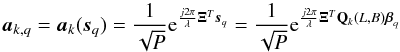 (9)where Ξ is a 3 × P matrix containing the positions of the P receiving elements. We introduced a scaling by
  as a normalization constant such that ∥ ak(sq) ∥ = 1. The entries of the array response vector are connected to the Fourier transform coefficients that are familiar in radio astronomy models.
Assuming an array that is otherwise calibrated, the received antenna signals yk [n] can be modeled as ![Mathematical equation: \begin{eqnarray} \label{eq:samplemodel} \by_k[n]=\bA_k\bx[n]+\bn_k[n], \qquad n = 1, \cdots, N \end{eqnarray}](/articles/aa/full_html/2016/04/aa26214-15/aa26214-15-eq67.png) (10)where Ak is a P × Q matrix whose columns are the array response vectors [Ak] q = ak,q, x [n] is a Q × 1 vector representing the signals from the sky, and nk [n] is a P × 1 vector modeling the noise.
(10)where Ak is a P × Q matrix whose columns are the array response vectors [Ak] q = ak,q, x [n] is a Q × 1 vector representing the signals from the sky, and nk [n] is a P × 1 vector modeling the noise.
From the data, the system estimates covariance matrices of the input vector at each snapshot k = 1,··· ,K, as ![Mathematical equation: \begin{equation} \bRh_{k} = \frac{1}{N} \sum_{n=1}^{N} \by_k[n]\by_k[n]^H, \qquad k = 1, \cdots, K \,. \end{equation}](/articles/aa/full_html/2016/04/aa26214-15/aa26214-15-eq76.png) (11)Since the received signals and noise are Gaussian, these covariance matrix estimates form sufficient statistics for the imaging problem (Leshem & van der Veen 2000). The covariance matrices are given by
(11)Since the received signals and noise are Gaussian, these covariance matrix estimates form sufficient statistics for the imaging problem (Leshem & van der Veen 2000). The covariance matrices are given by  (12)for which the model is
  (13)where Σ = ℰ { xxH } and
  are the source and noise covariance matrices, respectively. We have assumed that sky sources are stationary, and if we also assume that they are independent, we can model Σ = diag(σ) where
  (14)represents the intensity of the sources. To connect the covariance data model (13)to language more familiar to radio astronomers, let us take a closer look at the elements of the matrix Rk. Temporarily ignoring the noise covariance matrix Rn,k, we note that
 ![Mathematical equation: \begin{eqnarray} [\bR_k]_{ij}&=& \frac{1}{P} \sum_{q=1}^Q \sigma_q a_{kqi} a_{kqi}^* \notag \\ &=&\frac{1}{P}\sum_{q=1}^Q \sigma_q {\rm e}^{j\frac{2 \pi}{\lambda} (\bxi_i-\bxi_j)^T\bs_q}\notag \\ &=&\frac{1}{P}\sum_{q=1}^Q \sigma_q {\rm e}^{j\frac{2 \pi}{\lambda} \left [(x_i-x_j)l_q + (y_i-y_j)m_q+(z_i-z_j)\sqrt{1-l^2_q-m^2_q} \right].} \end{eqnarray}](/articles/aa/full_html/2016/04/aa26214-15/aa26214-15-eq85.png) (15)If we define
(15)If we define ![Mathematical equation: \hbox{$\frac{1}{\lambda}[x_i-x_j,y_i-y_j,z_i-z_j]^T = [u_{ij},v_{ij},w_{ij}]^T$}](/articles/aa/full_html/2016/04/aa26214-15/aa26214-15-eq86.png) , then we can write [Rk] ij ≡ V(uij,vij,wij), where V(u,v,w) is the visibility function, and (u,v,w) are the spatial frequencies (Leshem et al. 2000). In other words, the entries of the covariance matrix Rk are samples of the visibility function at a given frequency and time arranged in a matrix, and Eq. (13)represents the measurement equation in matrix form.
, then we can write [Rk] ij ≡ V(uij,vij,wij), where V(u,v,w) is the visibility function, and (u,v,w) are the spatial frequencies (Leshem et al. 2000). In other words, the entries of the covariance matrix Rk are samples of the visibility function at a given frequency and time arranged in a matrix, and Eq. (13)represents the measurement equation in matrix form.
We can write this equation in several other ways. By vectorizing both sides of (13)and using the properties of Kronecker products (4), we obtain 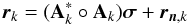 (16)where \begin{lxirformule}$\br_k=\vect(\bR_k)$\end{lxirformule} and rn,k = vect(Rn,k). After stacking the vectorized covariances for all of the snapshots, we obtain
 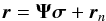 (17)where
 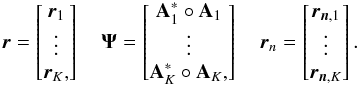 (18)Similarly, we vectorize and stack the sample covariance matrices as
  (19)This collects all the available covariance data into a single vector.
Alternatively, we can use the independence between the time samples to write the aggregate data model as  (20)where
3. The imaging problem
Using the data model (17), the imaging problem is to find the intensity, σ, of the sources, along with their directions represented by the matrices Ak, from given sample covariance matrices  . As the source locations are generally unknown, this is a complicated (nonlinear) direction-of-arrival estimation problem.
The usual approach in radio astronomy is to define a grid for the image and to assume that each pixel (grid location) contains a source. In this case the source locations are known, and estimating the source intensities is a linear problem, but for high-resolution images the number of sources may be very large. The resulting linear estimation problem is often ill-conditioned unless additional constraints are posed.
3.1. Gridded imaging model
After defining a grid for the image and assuming that a source exists for each pixel location, let I (rather than Q) denote the total number of sources (pixels), σ an I × 1 vector containing the source intensities, and Ak (k = 1,··· ,K) the P × I array response matrices for these sources. The Ak are known, and σ can be interpreted as a vectorized version of the image to be computed.(To distinguish the gridded source locations and source powers from the “true” sources, we later denote parameters and variables that depend on the Q true sources by a tilde.)
For a given observation  , image formation amounts to the estimation of σ. For a sufficiently fine grid, σ approximates the solution of the discrete source model. However, as we discuss later, working in the image domain leads to a gridding-related noise floor. This is solved by fine adaptation of the location of the sources and estimation of the true locations in the visibility domain.
A consequence of using a discrete source model in combination with a sequential source-removing technique such as CLEAN is the modeling of extended structures in the image by many point sources. As we discuss in Sect. 6, this also holds for the algorithms proposed in this paper.
3.2. Unconstrained least squares image
If we ignore the term rn, then Eq. (17)directly leads to least squares (LS) and weighted least squares (WLS) estimates of σ (Wijnholds & van der Veen 2008). In particular, solving the imaging problem with LS leads to the minimization problem  (23)where the normalization factor 2K is introduced to simplify the expression for the gradient and does not affect the solution. It is straightforward to show that the solution to this problem is given by any σ that satisfies
  (24)where we define the “matched filter” (MF, also known as the classical “direct Fourier transform dirty image”) as
 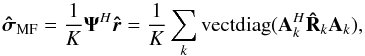 (25)and the deconvolution matrix HLS as
 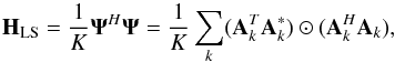 (26)where we have used the definition of Ψ from Eq. (18)(with tilde removed) and properties of the Kronecker and Khatri-Rao products. Similarly we can define the WLS minimization as
 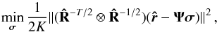 (27)where the weighting assumes Gaussian distributed observations. The weighting improves the statistical properties of the estimates, and
  is used instead of R because it is available and asymptotically gives the same optimal results, i.e., convergence to maximum likelihood estimates (Ottersten et al. 1998). The solution to this optimization is similar to the solution to the LS problem and is given by any σ that satisfies
  (28)where
 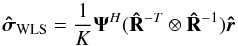 (29)is the “WLS dirty image” and
 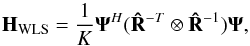 (30)is the associated deconvolution operator.
A connection to beamforming is obtained as follows. The ith pixel of the “Matched Filter” dirty image in Eq. (25) can be written as 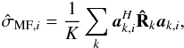 and if we replace
  by a more general “beamformer” wk,i, this can be generalized to a more general dirty image
 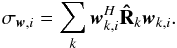 (31)Here, wk,i is called a beamformer because we can consider that it acts on the antenna vectors yk [n] as
 ![Mathematical equation: \hbox{$z_{k,i}[n] = \bw_{k,i}^H \by_k[n]$}](/articles/aa/full_html/2016/04/aa26214-15/aa26214-15-eq122.png) , where zk,i [n] is the output of the (direction-dependent) beamformer, and σw,i = ∑ kℰ { | zk,i | 2 } is interpreted as the total output power of the beamformer, summed over all snapshots. We encounter several such beamformers in the rest of the paper. Most of the beamformers discussed in this paper include the weighted visibility vector (R− T ⊗ R-1)r. The relation between this weighting and more traditional weighting techniques, such as natural and robust weighting, is discussed in Appendix A.
, where zk,i [n] is the output of the (direction-dependent) beamformer, and σw,i = ∑ kℰ { | zk,i | 2 } is interpreted as the total output power of the beamformer, summed over all snapshots. We encounter several such beamformers in the rest of the paper. Most of the beamformers discussed in this paper include the weighted visibility vector (R− T ⊗ R-1)r. The relation between this weighting and more traditional weighting techniques, such as natural and robust weighting, is discussed in Appendix A.
3.3. Preconditioned weighted least squares image
If Ψ has full column rank, then HLS and HWLS are non-singular and a unique solution to LS and WLS exists; for example, the solution to Eq. (24)becomes 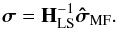 (32)Unfortunately, if the number of pixels is large, then HLS and HWLS become ill-conditioned or even singular, so that Eqs. (24)and (28)have an infinite number of solutions (Wijnholds & van der Veen 2008). Generally, we need to improve the conditioning of the deconvolution matrices and to find appropriate regularizations.
One way to improve the conditioning of a matrix is to apply a preconditioner. The most widely used and simplest one is the Jacobi preconditioner (Barrett et al. 1994), which for any matrix M, is given by [diag(M)] -1. Let DWLS = diag(HWLS), then by applying this preconditioner to HWLS we obtain ![Mathematical equation: \begin{equation} \label{eq:imagingeqwlspre} [\bD_{\text{WLS}}^{-1}\HWLS]\bsigma=\bD_{\text{WLS}}^{-1}\SWLSDI . \end{equation}](/articles/aa/full_html/2016/04/aa26214-15/aa26214-15-eq131.png) (33)We take a closer look at
(33)We take a closer look at  for the case where K = 1. In this case,
 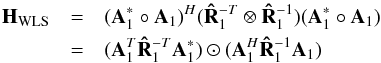 and
and 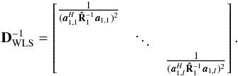 This means that
 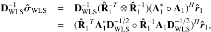 which is equivalent to a dirty image that is obtained by applying a beamformer of the form
  (34)to both sides of
  and stacking the results,
  , of each pixel into a vector. This beamformer is known in array processing as the minimum variance distortionless response (MVDR) beamformer (Capon 1969), and the corresponding dirty image is called the MVDR dirty image and was introduced in the radio astronomy context in Leshem & van der Veen (2000). This shows that the preconditioned WLS image (motivated by its connection to the maximum likelihood) is expected to exhibit the features of high-resolution beamforming associated with the MVDR. Examples of such images are shown in Sect. 6.
3.4. Bounds on the image
Another approach to improving the conditioning of a problem is to introduce appropriate constraints on the solution. Typically, image formation algorithms exploit external information regarding the image in order to regularize the ill-posed problem. For example, maximum entropy techniques (Frieden 1972; Gull & Daniell 1978) impose a smoothness condition on the image, while the CLEAN algorithm (Högbom 1974) exploits a point source model wherein most of the image is empty, and this has recently been connected to sparse optimization techniques (Wiaux et al. 2009).
A lower bound on the image is almost trivial: each pixel in the image represents the intensity at a certain direction, so is non-negative. This leads to a lower bound σ ≥ 0. Such a non-negativity constraint has been studied, for example, in (Briggs 1995), resulting in a non-negative LS (NNLS) problem  (35)A second constraint follows if we also know an upper bound γ such that σ ≤ γ, which will bound the pixel intensities from above. We propose several choices for γ.
By closer inspection of the ith pixel of the MF dirty image  , we note that its expected value is given by
  Using
Using  (36)and the normalization
  , we obtain
  (37)where
 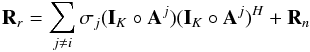 (38)is the contribution of all other sources and the noise. We note that Rr is positive-(semi)definite. Thus, Eq. (37) implies σMF,i ≥ σi which means that the expected value of the MF dirty image forms an upper bound for the desired image, or
  (39)Using the relation between the MF dirty image and beamformers as discussed in Sect. 3.2, we answer the following question: What is the tightest upper bound for σi that we can construct using linear beamforming?
This question can be translated into an optimization problem and a closed form solution (Appendix B) exists: 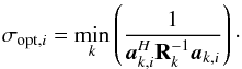 (40)Here σopt,i is the tightest upper bound, and the beamformer that achieves this bound is called the adaptive selective sidelobe canceller (ASSC; Levanda & Leshem 2013).
One problem with using this result in practice is that σopt,i depends on a single snapshot. Actual dirty images are based on the sample covariance matrix , so they are random variables. If we use a sample covariance matrix instead of the true covariance matrix R in Eq. (40), the variance of the result can be unacceptably large. An analysis of this problem and various solutions for it are discussed in Levanda & Leshem (2013).
To reduce the variance we tolerate an increase of the bound with respect to the tightest upper bound, however, we would like our result to be tighter than the MF dirty image. It can be shown that the MVDR dirty image defined as 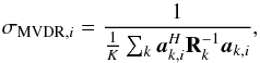 (41)satisfies σi ≤ σMVDR,i ≤ σMF,i and produces a very tight bound (see Appendix B for the proof). This leads to the following constraint
  (42)Interestingly, for K = 1 the MVDR dirty image is the same image as we obtained earlier by applying a Jacobi preconditioner to the WLS problem.
3.5. Estimation of the upper bound from noisy data
The upper bounds (39)and (42) assume that we know the true covariance matrix R. However, in practice we only measure , which is subject to statistical fluctuations. Choosing a confidence level of six times the standard deviation of the dirty images ensures that the upper bound will hold with a probability of 99.9%.
This leads to an increase in the upper bound by a factor 1 + α where α> 0 is chosen such that  (43)Similarly, for the MVDR dirty image, the constraint based on is
  (44)where
  (45)is an unbiased estimate of the MVDR dirty image, and
  (46)is a bias correction constant. With some algebra the unbiased estimate can be written in vector form as
  (47)where
 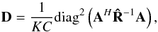 (48)and
  (49)The exact choice of α and C are discussed in Appendix C.
3.6. Constrained least squares imaging
Now that we have lower and upper bounds on the image, we can use these as constraints in the LS imaging problem to provide a regularization. The resulting constrained LS (CLS) imaging problem is 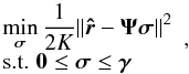 (50)where γ can be chosen either as γ = σMF for the MF dirty image or γ = σMVDR for the MVDR dirty image (or their sample covariance based estimates given by formulae (43)and (44)).
The improvements to the unconstrained LS problem that were discussed in Sect. 3.2 are still applicable. The extension to WLS leads to the cost function
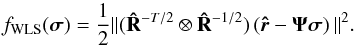 (51)The constrained WLS problem is then given by
 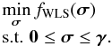 (52)We also recommend including a preconditioner that, as shown in Sect. 3.3, relates the WLS to the MVDR dirty image. However, because of the inequality constraints, (52)does not have a closed form solution, and it is solved by an iterative algorithm. To have the relation between WLS and MVDR dirty image during the iterations, we introduce a change of variable of the form
  , where
  is the new variable for the preconditioned problem and the diagonal matrix D is given in (48). The resulting constrained preconditioned WLS (CPWLS) optimization problem is
 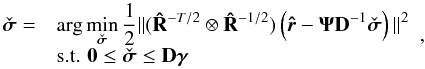 (53)and the final image is found by setting
  . (Here we use D as a positive diagonal matrix so that the transformation to an upper bound for is correct.) Interestingly, the dirty image that follows from the (unconstrained) WLS part of the problem is given by the MVDR image
  in (47).
4. Constrained optimization using an active set method
The constrained imaging formulated in the previous section requires the numerical solution of the optimization problems (50) or (53). The problem is classified as a positive definite quadratic program with simple bounds, this is a special case of a convex optimization problem with linear inequality constraints, and we can follow standard approaches to find a solution (Gill et al. 1981; Boyd & Vandenberghe 2004).
For an unconstrained optimization problem, the gradient of the cost function calculated at the solution must vanish. If we are not yet at the optimum in an iterative process, the gradient is used to update the current solution. For constrained optimization, the constraints are usually added to the cost function using (unknown) Lagrange multipliers that need to be estimated along with the solution. At the solution, part of the gradient of the cost function is not zero but related to the nonzero Lagrange multipliers. For inequality constraints, the sign of the Lagrange multipliers plays an important role.
As we show here, these characteristics of the solution (based on the gradient and the Lagrange multipliers) can be used to develop an algorithm called the active set method, which is closely related to the sequential source removing techniques such as CLEAN.
In this section, we use the active set method to solve the constrained optimization problem.
4.1. Characterization of the optimum
Let  be the solution to the optimization problem (50) or (53). An image is called feasible if it satisfies the bounds σ ≥ 0 and −σ ≥ −γ. At the optimum, some pixels may satisfy a bound with equality, and these are called the “active” pixels.
We use the following notation. For any feasible image σ, let 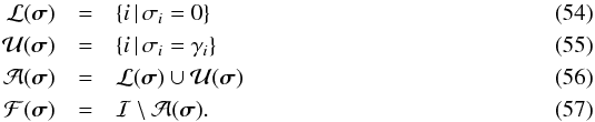 Here, ℐ = { 1,··· ,I } is the set of all pixel indices; ℒ(σ) is the set where the lower bound is active, i.e., the pixel value is 0;
  is the set of pixels that attain the upper bound;
  is the set of all pixels where one of the constraints is active. These are the active pixels. The free set ℱ(σ) is the set of pixels i, which have values strictly between 0 and γi. Furthermore, for any vector v = [vi], let vℱ correspond to the subvector with indices i ∈ ℱ, and similarly define vℒ and
  . We write
  .
.
Let be the optimum, and let  be the gradient of the cost function at this point. Define the free sets and active sets
  at . We can write
 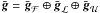 . Associated with the active pixels of is a vector
  of Lagrange multipliers. Optimization theory (Gill et al. 1981) tells us that the optimum is characterized by the following conditions:
 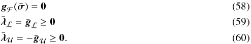 Thus, the part of the gradient corresponding to the free set is zero, but the part of the gradient corresponding to the active pixels is not necessarily zero. Since we have simple bounds, this part becomes equal to the Lagrange multipliers
  and
and  (the negative sign is caused by the condition
  ). The condition λ ≥ 0 is crucial: a negative Lagrange multiplier would indicate that there is a feasible direction of descent p for which a small step in that direction,
  , has a lower cost and still satisfies the constraints, thus contradicting optimality of (Gill et al. 1981).
“Active set” algorithms consider that if the true active set at the solution is known, the optimization problem with inequality constraints reduces to an optimization with equality constraints,  (61)Since we can substitute the values of the active pixels into σ, the problem becomes a standard unconstrained LS problem with a reduced dimension: only
  needs to be estimated. Specifically, for CLS the unconstrained subproblem is formulated as
  (62)where
  (63)Similarly, for CPWLS we have
  (64)where
  (65)In both cases, closed form solutions can be found, and we discuss a suitable Krylov-based algorithm for this in Sect. 5.
As a result, the essence of the constrained optimization problem is to find ℒ,  , and ℱ. In the literature, algorithms for this are called “active set methods”, and we propose a suitable algorithm in Sect. 4.3.
4.2. Gradients
We first derive expressions for the gradients required for each of the unconstrained subproblems (62) and (64). Generically, a WLS cost function (as function of a real-valued parameter vector θ) has the form  (66)where G is a Hermitian weighting matrix and β is a scalar. The gradient of this function is
  (67)For LS we have θ = σ,
  ,
,  , and G = I. This leads to
  (68)For PWLS,
  ,
,  ,
,  , and
, and  . Substituting these into Eq. (67), we obtain
  (69)where
  (70)and we used Eq. (47).
An interesting observation is that the gradients can be interpreted as residual images obtained by subtracting the dirty image from a convolved model image. At a later point, this will allow us to relate the active set method to sequential source removing techniques.
4.3. Active set methods
In this section, we describe the steps needed to find the sets ℒ, and, ℱ, and the solution. We follow the template algorithm proposed in Gill et al. (1981). The algorithm is an iterative technique where we gradually improve on an image. Let the image at iteration j be denoted by σ(j) where j = 1,2,··· , and we always ensure this is a feasible solution (satisfies 0 ≤ σ(j) ≤ γ). The corresponding gradient is the vector g = g(σ(j)), and the current estimate of the Lagrange multipliers λ is obtained from g using (59) and (60). The sets ℒ, , and ℱ are current estimates that are not yet necessarily equal to the true sets.
If this image is not yet the true solution, it means that one of the conditions in Eqs. (58)−(60) is violated. If the gradient corresponding to the free set is not yet zero (gℱ ≠ 0), then this is remedied by recomputing the image from the essentially unconstrained subproblem (61). It may also happen that some entries of λ are negative. This implies that we do not yet have the correct sets ℒ, , and ℱ. Suppose λi< 0. The connection of λi to the gradient indicates that the cost function can be reduced in that dimension without violating any constraints (Gill et al. 1981), at the same time making the pixel no longer active. Thus we remove the ith pixel from the active set, add it to the free set, and recompute the image with the new equality constraints using Eq. (61). As discussed later, a threshold ϵ is needed in the test for the negativity of λi, therefore this step is called the “detection problem”.
Table 1 summarizes the resulting active set algorithm and describes how the solution z to the subproblem is used at each iteration. Some efficiency is obtained by not computing the complete gradient g at every iteration, but only the parts corresponding to  , when they are needed. For the part corresponding to ℱ, we use a flag that indicates whether gℱ is zero or not.
Constrained LS imaging using active sets.
The iterative process is initialized in line 1. This can be done in many ways. As long as the initial image lies within the feasible region (0 ≤ σ(0) ≤ γ), the algorithm will converge to a constrained solution. We can simply initialize by σ(0) = 0.
Line 3 is a test for convergence, corresponding to the conditions (58)−(60). The loop is followed while any of the constraints is violated.
If gℱ is not zero, then the unconstrained subproblem (61) is solved in line 5. If this solution z satisfies the feasibility constraints, then it is kept, the image is updated accordingly, and the gradient is estimated at the new solution (only λmin = min(λ) is needed, along with the corresponding pixel index).
If z is not feasible, then in lines 12−16 we try to move in the direction of z as far as possible. The direction of descent is  , and the update will be
  , where μ is a non-negative step size. The ith pixel will hit a bound if either
  or
or  ; i.e., if
  (71)(μi is non-negative). Then the maximal feasible step size towards a constraint is given by μmax = min(μi) for i ∈ ℱ. The corresponding pixel index is removed from ℱ and added to ℒ or .
If in line 3 the gradient satisfied gℱ = 0 but a Lagrange multiplier is negative, we delete the corresponding constraint and add this pixel index to the free set (line 20). After this, the loop is entered again with the new constraint sets.
If we initialize the algorithm with σ(0) = 0, then all pixel indices will be in the set ℒ, and the free set is empty. During the first iteration, σℱ remains empty but the gradient is computed (line 9). Equations (68)and (69)show that it will be equal to the negated dirty image. Thus the minimum of the Lagrange multipliers λmin will be the current strongest source in the dirty image, and it will be added to the free set when the loop is entered again. This shows that the method as described above will lead to a sequential source removal technique similar to CLEAN. In particular, the PWLS cost function (69)relates to LS-MVI (Ben-David & Leshem 2008), which applies CLEAN-like steps to the MVDR dirty image.
In line 3, we try to detect whether a pixel should be added to the free set (λmin< 0). We note that λ follows from the gradient, (68)or (69), which is a random variable. We should avoid the occurrence of a “false alarm”, because it will lead to overfitting the noise. Therefore, the test should be replaced by λmin< −ϵ, where ϵ> 0 is a suitable detection threshold. Because the gradients are estimated using dirty images, they share the same statistics (the variance of the other component in Eqs. (68)and (69)is much smaller). To reach a desired false alarm rate, we propose to choose ϵ proportional to the standard deviation of the ith pixel on the corresponding dirty image for the given cost function. (How to estimate the standard deviation of the dirty images and the threshold is discussed in Appendix C.) Choosing ϵ to be six times the standard deviation ensures a false alarm of < 0.1% over the complete image.
The use of this statistic improves the detection and thus the estimates greatly, however the correct detection also depends on the quality of the estimates in the previous iterations. If a strong source is off-grid, the source is usually underestimated, and this leads to a biased estimation of the gradient and the Lagrange multipliers, which in turn leads to including pixels that are not real sources. In the next section we describe one possible solution for this case.
4.4. Strong off-grid sources
In this section, we use a tilde to indicate “true” source parameters (as distinguished from the gridded source model); for example,  indicates the vector with the true source intensities, and
  the corresponding diagonal matrix,
  indicates their array response vectors and
  the corresponding matrix. The versions without tilde refers to the I gridded sources.
The mismatch between Ψ and the unknown  results in underestimating source intensities, which means that the remaining contribution of that source produces bias and possible artifacts in the image. To achieve high dynamic ranges, we suggest finding a grid correction for the pixels in the free set ℱ.
Let ak,i have the same model as with βi pointing toward the center of the ith pixel. When a source is within a pixel but not exactly in the center, we can model this mismatch as 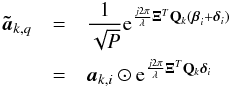 where
where  and i ∈ ℱ. Because both βi and
  are 3 × 1 unit vectors, each only has two degrees of freedom. This means that we can parameterize the unknowns for the grid-correcting problem using coefficients δ1,i and δi,2. We assume that when a source is added to the free set, its actual position is very close to the center of the pixel on which it was detected. This means that δ1,i and δi,2 are within the pixel’s width, denoted by W, and height, denoted by H. In this case we can replace Eq. (61)by a nonlinear constrained optimization,
 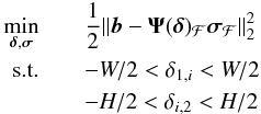 (72)where Ψ(δ)ℱ contains only the columns corresponding to the set ℱ, δj is a vector obtained by stacking δi,j for j = 1,2, and
  (73)This problem can also be seen as a direction of arrival (DOA) estimation that is an active research area and beyond the scope of this paper. A good review of DOA mismatch correction for MVDR beamformers can be found in Chen & Vaidyanathan (2007), and Gu & Leshem (2012) proposed a correction method that is specifically applicable to the radio astronomical context.
Besides solving formula (72)instead of Eq. (61)in line 5 of the active set method, we also need to update the upper bounds and the standard deviations of the dirty images at the new pixel positions that are used in the other steps (e.g., lines 3, 6, and 13); the rest of the steps remain the same. Because we have a good initial guess to where each source in the free set is, we propose a Newton-based algorithm to do the correction.
4.5. Boxed imaging
A common practice in image deconvolution techniques like CLEAN is to use a priori knowledge and to narrow the search area for the sources to a certain region of the image, called CLEAN boxes. Because the contribution of the sources (if any) outside these boxes is assumed to be known, we can subtract them from the data such that we can assume that the intensity outside the boxes is zero.
To include these boxes in the optimization process of the active set algorithm, it is sufficient to make sure that the value of the pixels not belonging to these boxes do not change and remain zero. This is equivalent to replacing Ψ with Ψℬ, where ℬ is the set of indices belonging to the boxes, before we start the optimization process. However, as we explain in the next section, we avoid storing the matrix Ψ in memory by exploiting its Khatri-Rao structure. We address this implementation issue by replacing Eq. (57)with  (74)which makes certain that the values of the elements outside of the boxes do not change. This has the same effect as removing the columns not belonging to ℬ from Ψ. Of course we have to make sure that these values are initialized to zero. By choosing σ(0) = 0, this is automatically the case. The only problem with this approach is that the values outside the box remain in the set ℒ that is used for estimating the Lagrange variables, resulting in expensive calculations that are not needed. This problem is easily solved by calculating the gradient only for the pixels belonging to ℬ. The a priori non-zero values of the pixels (that were not in the boxes and were removed from the data) are added to the solution when the optimization process is finished.
5. Implementation using Krylov subspace-based methods
From the active-set methods described in the previous section, we know that we need to solve Eqs. (62)or (64)at each iteration. In this section we describe how to achieve this efficiently without the need to store the whole convolution matrix in memory.
During the active-set updates, we need to solve linear equations of the form Mx = b. However, there are cases where we do not have direct access to the elements of the matrix M. This can happen, for example, when M is too large to fit in memory. There are also cases where M (or MH) are implemented as subroutines that produce the result of the matrix vector multiplication Mv for some input vector v. For example, for M = Ψ the operation ΨHv generates a dirty image. An equivalent (and maybe optimized) implementation of such imaging subroutine might already be available to the user. In these scenarios it is necessary or beneficial to be able to solve the linear systems, using only the available matrix vector multiplication or the equivalent operator. A class of iterative solvers that can solve a linear system by only having access to the result of the multiplications with the matrix M are the Krylov subspace-based methods.
To illustrate the idea behind Krylov subspace-based methods, we assume that M is a square and non-singular matrix. In this case there exists a unique solution for x that is given by x = M-1b. Using the minimum polynomial of a matrix we can write 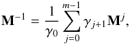 where for a diagonalizable matrix M, m is the number of distinct eigenvalues (Ipsen & Meyer 1998). Using this polynomial expansion we have for our solution
 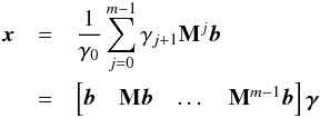 where
where ![Mathematical equation: \begin{eqnarray*} \bgamma=\frac{1}{\gamma_0}[\gamma_1, \dots, \gamma_m]^T, \end{eqnarray*}](/articles/aa/full_html/2016/04/aa26214-15/aa26214-15-eq300.png) and
and ![Mathematical equation: \hbox{$\MCK_m(\bM,\bb)=[\bb, \bM\bb, \dots, \bM^{m-1}\bb]$}](/articles/aa/full_html/2016/04/aa26214-15/aa26214-15-eq301.png) is called the Krylov subspace of M and b. Krylov subspace-based methods compute
is called the Krylov subspace of M and b. Krylov subspace-based methods compute  iteratively, for n = 1,2,.. and find an approximate for x by means of a projection on this subspace. Updating the subspace only involves a matrix-vector multiplication of the form Mv.
In cases where M is singular or where it is not a square matrix, another class of Krylov-based algorithms can be used that is related to bidiagonalization of the matrix M. The rest of this section describes the idea behind the Krylov-based technique LSQR and the way this helps more efficient implementation of a linear solver for our imaging algorithm.
5.1. Lanczos algorithm and LSQR
When we are solving CLS or PWLS, we need to solve a problem of the form  as the first step in the active-set iterations; for example, in Eq. (62)M = Ψℱ. It does not have to be a square matrix, and usually it is ill-conditioned, especially if the number of pixels is large. In general we can find a solution for this problem by first computing the singular value decomposition (SVD) of M as
  (75)where U and V are unitary matrices, and S is a diagonal matrix with positive singular values. Then the solution x to min ∥ b−Mx ∥ 2 is found by solving for y in
  (76)followed by setting
  (77)Solving the LS problem with this method is expensive in both number of operations and memory usage, especially if the matrices U and V are not needed after finding the solution. As we see below, looking at another matrix decomposition helps us to reduce these costs. For the rest of this section we use the notation given by (Paige & Saunders 1982).
The first step in this approach for solving LS problem is to reduce M to a lower bidiagonal form as follows  (78)where B is a bidiagonal matrix of the form
 ![Mathematical equation: \begin{equation} \bB=\left[\begin{array}{cccc|c} \alpha_1 & & & & \\ \beta_2&\alpha_2 & & & \\ &\ddots&\ddots & & \\ & & \beta_r&\alpha_r &\\ \hline & & & & \zeros\\ \end{array}\right],\\ \end{equation}](/articles/aa/full_html/2016/04/aa26214-15/aa26214-15-eq317.png) (79)where r = rank(M) = rank(B) and U,V are unitary matrices (different than in Eq. (75)). This representation is not unique, and without loss of generality we could choose U to satisfy
(79)where r = rank(M) = rank(B) and U,V are unitary matrices (different than in Eq. (75)). This representation is not unique, and without loss of generality we could choose U to satisfy  (80)where β1 = ∥ b ∥ 2 and e1 is a unit norm vector with its first element equal to one.
Using B, forward substitution gives the LS solution efficiently by solving y in  (81)followed by
  (82)Using forward substitution we have
  followed by the recursion,
  for n = 1,...,M where M<r is the iteration at which ∥ MH(Mxn−b) ∥ 2 vanishes within the desired precision. We can combine the bidiagonalization and solving for x and avoid extra storage needed for saving B, U, and V. One such algorithm is based on a Krylov subspace method called the Lanczos algorithm (Golub & Kahan 1965). We first initialize with
 ![Mathematical equation: \begin{eqnarray} \label{eq:initbeta} \beta_1&=&\|\bb\|_2\\[3mm] \label{eq:initu} \bu_1&=&\frac{\bb}{\beta_1}\\[3mm] \alpha_1&=&\|\bM^H\bu_1\|_2\\[3mm] \bv_1&=& \frac{\bM^H\bu_1}{\alpha_1}\cdot \end{eqnarray}](/articles/aa/full_html/2016/04/aa26214-15/aa26214-15-eq330.png) The iterations are then given by
The iterations are then given by ![Mathematical equation: \begin{eqnarray} \label{eq:lanczos} \begin{array}{l l} \beta_{n+1}&= \|\bM\bv_{n}-\alpha_{n}\bu_{n}\|_2\\[3mm] \bu_{n+1}&=\frac{1}{\beta_{n+1}} (\bM\bv_n-\alpha_n\bu_n) \\[3mm] \alpha_{n+1}&=\|\bM^H\bu_{n+1}-\beta_{n+1}\bv_{n}\|_2 \\[3mm] \bv_{n+1}&=\frac{1}{\alpha_{n+1}} (\bM^H\bu_{n+1}-\beta_{n+1}\bv_n) \end{array} \end{eqnarray}](/articles/aa/full_html/2016/04/aa26214-15/aa26214-15-eq331.png) (91)for n = 1,2,...,M, where
(91)for n = 1,2,...,M, where  . This provides us with all the parameters needed to solve the problem.
However, because of finite precision errors, the columns of U and V found in this way lose their orthogonality as we proceed. To prevent this error propagation into the final solution x, different algorithms, such as conjugate gradient (CG), MINRES, and LSQR, have been proposed. The exact updates for xn and stopping criteria to find M depend on the choice of algorithm used and therefore are not included in the iterations above.
An overview of Krylov subspace-based methods is given by (Choi 2006, p.91). This study shows that LSQR is a good candidate for solving LS problems when we are dealing with an ill-conditioned and non-square matrix. For this reason we use LSQR to solve Eqs. (62)or (64). Because the remaining steps during the LSQR updates are a few scalar operations and do not have a large impact on the computational complexity of the algorithm, we do not go into the details(see Paige & Saunders 1982).
In the next section we discuss how to use the structure in M to avoid storing the entire matrix in memory and how to parallelize the computations.
5.2. Implementation
During the active set iteration we need to solve Eqs. (62)and (64)where the matrix M in LSQR is replaced by Ψℱ and (R− T/ 2 ⊗ R− 1/2)(ΨD-1)ℱ, respectively. Because Ψ has a Khatri-Rao structure and selecting and scaling a subset of columns does not change this, Ψℱ and (ΨD-1)ℱ also have a Khatri-Rao structure. Here we show how to use this structure to implement Eqs. (91)in parallel and with less memory usage.
The only time the matrix M enters the algorithm is via the matrix-vector multiplications Mvn and MHun + 1. As an example we use M = Ψℱ for solving Eq. (62). Let kn = Ψℱvn. We partition kn as Ψ into  (92)Using the definition of Ψ in Eq. (18), the operation kn = Ψℱvn could also be performed using
  (93)and subsequently we set
  (94)This process can be highly parallelized because of the independence between the correlation matrices of each time snapshot. The matrix Kk,n can then be used to find the updates in Eqs. (91).
The operation MHu in Eq. (91)is implemented in a similar way. Using the beamforming approach (similar to Sect. 3.4), this operation can also be done in parallel for each pixel and each snapshot. In both cases the calculations can be formulated as correlations and beamforming of parallel data paths, which means that efficient hardware implementations are feasible. Also we can consider traditional LS or WLS solutions as a special case when all the pixels belong to the free set, which means that those algorithms can also be implemented efficiently in hardware in the same way. During the calculations we work with a single beamformer at the time, and the matrix Ψ need not to be precalculated and stored in memory. This makes it possible to apply image formation algorithms for large images when there is a memory shortage.
The computational complexity of the algorithm is dominated by the transformation between the visibility domain and image domain (correlation and beamforming). The dirty image formation and correlation have a complexity of O(KP2I). This means that the worst-case complexity of the active set algorithm is O(TMKP2I) where T is the number of active set iterations and M the maximum number of Krylov iterations. A direct implementation of CLEAN for solving the imaging problem presented in Sect. 3 in a similar way would have a complexity of O(TKP2I). The proposed algorithm is therefore order M times more complex, essentially because it recalculates the flux for all the pixels in the free set, while CLEAN only estimates the flux of a newly added pixel. Considering that (for a well-posed problem) solving Mx = b using LSQR is algebraically equivalent to solving MHMx = MHb using CG (Fong 2011), we can use the convergence properties of CG (Demmel 1997) to obtain an indication of the required number of Krylov iterations M. It is found that M is on the order  where card(ℱ) is the cardinality of the free set, which is equal to the number of pixels in the free set.
In practice, many implementations of CLEAN use the FFT instead of a DFT (matched filter) for calculating the dirty image. Extending the proposed method to use similar techniques is possible and will be presented in future works.
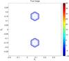 |
Fig. 1 Contoured true source on dB scale. |
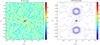 |
Fig. 2 Contoured dirty images on dB scale. a) MF dirty image. b) MVDR dirty image. |
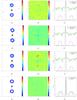 |
Fig. 3 Extended source simulations. Units for the first and third columns are in dB. Linear scale is used for residual images (second column). a) CLEAN Image. b) CLEAN Residual image. c) CLEAN cross-section. d) Solution of CLS + MF. e) Residual image for CLS + MF. f) Cross-section for CLS + MF. g) Solution of CLS + MVDR. h) Residual image for CLS + MVDR. i) Cross-section for CLS image + MVDR. j) CPWLS image. k) CPWLS residual image. l) MVDR dirty image and CPWLS cross-section. |
6. Simulations
The performance of the proposed methods were evaluated using simulations. Because the active-set algorithm adds a single pixel to the free set at each step, it is important to investigate the effect of this procedure on extended sources and noise. For this purpose, in our first simulation set-up we used a high dynamic range simulated image with a strong point source and two weaker extended sources in the first part of the simulations. In a second set up, we made a full sky image using sources from the 3C catalog.
Following the discussion in Sect. 4.2, we defined the residual image for CLS and CLEAN as  and for CPWLS, we used
  where we assumed we know the noise covariance matrix Rn.We also defined the reconstruction S/N on the image in dB scale as
 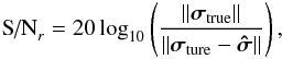 where σtrue is the true image and
  is the reconstructed image.
6.1. Extended sources
An array of 100 dipoles (P = 100) with random distribution was used with the frequency range of 58−90 MHz from which we simulated three equally spaced channels. Each channel has a bandwidth of 195 kHz and was sampled at Nyquist rate. These specifications are consistent with the LOFAR telescope in LBA mode (van Haarlem et al. 2013). LOFAR uses one-second snapshots, and we did the simulation using only two snapshots, i.e., K = 2. We used spectrally white sources for the simulated frequency channels, which allowed us to extend the data model to one containing all frequency data by simply stacking the individual for each frequency into a single vector. Likewise, we stacked the individual Ψ into a single matrix. Since the source intensity vector σ is common for all frequencies, the augmented data model has the same structure as before.
The simulated source is a combination of a strong point source with intensity 40 dB and two extended structures with intensities of 0 dB. The extended structures are composed of from seven nearby Gaussian-shaped sources, one in the middle and six on a hexagon around it. (This configuration was selected to generate an easily reproducible example.) Figure 1 shows the simulated image on dB scale. The background noise level that was added is at −10 dB, which is also 10 dB below the extended sources. This is equivalent to a dynamic range of 40 dB and a minimum S/N of 10 dB.
Figures 2a and b show the matched filter and MVDR dirty images, respectively. The first column of Fig. 3 shows the final result of the CLEAN, CLS with the MF dirty image as upper bound, CLS with the MVDR dirty image as upper bound, and CPWLS with the MVDR dirty image as upper bound without the residual images. For each image, the extracted point sources were convolved with a Gaussian beam to smoothen the image. We used a Gaussian beam that has the same main beamwidth as the MF dirty image. The second column of Fig. 3 shows the corresponding residual images as defined before, and the last column shows a cross section parallel to the β2 axis going through the sources at the center of the image.
Remarks are:
-
As expected the MVDR dirty image has a much better dynamicrange (≈ 40 dB) and lower side-lobes compared to the MF dirty image (≈ 15 dB dynamic range).
-
Due to a better initial dirty image and upper bound, the CPWLS deconvolution gives a better reconstruction of the image.
-
The cross sections show the accuracy of the estimated intensities. This shows that not only the shape but also the magnitude of the sources are better estimated using CPWLS.
-
Using the MVDR upper bound for CLS improves the estimate, illustrating the positive effect of using a proper upper bound.
-
All algorithms manage to recover the intensity of the strong point source with high quality. The S/Nr for CLS and CLS with MVDR is highest at 62.8 dB then CLEAN and CPWLS with 62.6 and 58.4 dB, respectively. (Only the pixel corresponding to the strong source is used to calculate these S/Nr.)
-
CPWLS has the best performance in recovering the extended sources with S/Nr of 16.5 dB compared to 11.9 and 11.7 dB for CLEAN and CLS respectively. (The pixel corresponding to the strong source was removed for calculating these S/Nr.)
-
The residual image for CPWLS is almost two orders of magnitude lower than the residual images for CLEAN and CLS.
-
While the residual image of the CLS algorithm appears very similar to the CLEAN reconstruction, CLS can guarantee that these values are inside the chosen confidence interval of six standard deviations of each pixel, while CLEAN does not provide this guarantee.
6.2. Full sky with 3C sources
In a second simuation set-up, we constructed an all-sky image with sources from the 3C catalog. The array configuration is the same as before with the same number of channels and snapshots. A background noise level of 0 dB (with respect to 1 Jansky) is added to the sky.
We first checked which sources from the 3C catalog are visible at the simulated date and time. From these we chose 20 sources that represent the magnitude distribution on the sky and produce the highest dynamic range available in this catalog. Table 2 shows the simulated sources with corresponding parameters. The coordinates are the (l,m) coordinates at the first snapshot. Because the sources are not necessarily on the grid points, we combined the active set deconvolution with the grid corrections on the free set as described in Sect. 4.4.
Figure 4a shows the true and estimated positions for the detected sources. Because the detection mechanism was able to detect the correct number of sources, we have included the estimated fluxes in Table 2 for easier comparison. Figure 4b shows the full-sky MF dirty image. Figure 5a shows the final reconstructed image with the residual added to it (with grid corrections applied), and Fig. 5c shows the same result for CLEAN.
Remarks:
-
The active set algorithm with grid corrections automaticallystops after adding the correct number of sources based on thedetection mechanism we have incorporated in the active setmethod.
-
Because of the grid correction, no additional sources are added to compensate for incorrect intensity estimates on the grids.
-
All 20 sources are visible in the final reconstructed image, and no visible artifacts are added to the image.
-
CLEAN also produces a reasonable image with all the sources visible. However, a few hundred point sources have been detected during the CLEAN iteration, most of which are the result of the strong sources that are not on the grid. Some clear artifacts are introduced (as seen in the residual image) that are also the result of the incorrect subtraction of off-grid sources.
-
Figure 5b shows that the residual image using active set and grid corrections contains a “halo” around the position of the strong source–the residual image is not flat. In fact, the detection mechanism in the active set algorithm (with a threshold of 6 times the standard deviation) has correctly not considered this halo as a source. The halo is a statistical artifact due to finite samples and will be reduced in magnitude by longer observations with a rate proportional to
 .
. -
The CLEAN algorithm requires more than 100 sources to model the image. This is mainly because of the the strong off–grid source (Cassiopeia A). This illustrates that while CLEAN is less complex than the proposed method when the number of detected sources are equal, in practice CLEAN might need many more sources to model the same image.
Simulated sources from 3C catalog.
 |
Fig. 4 Point source simulations. a) Position estimates. b) Full sky MF dirty image in dB (with respect to 1 Jy). |
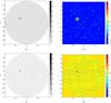 |
Fig. 5 Reconstructed images in dB (with respect to 1 Jy) scale and residual images on linear scale. a) Reconstructed image with grid correction plus residual image. b) Residual image using active set and grid correction. c) Reconstructed image with CLEAN plus residual image. d) Residual image using CLEAN. |
7. Conclusions
Based on a parametric model and constraints on the intensities, we have formulated image deconvolution as a weighted least squares optimization problem with inequality constraints. We first showed that the classical (matched filter) dirty image is an upper bound, but a much tighter upper bound is provided by the “MVDR dirty image”. The conditioning of the problem can be improved by a preconditioning step, which is also related to the MVDR dirty image.
Second, the constrained least squares problem was solved using an active-set-based method. The relation between the resulting method and sequential source removing techniques such as CLEAN was explained. The theoretical background of the active set methods can be used for deeper insight into how the sequential techniques work.In particular, the active set algorithm uses a detection threshold with a known false alarm, which can be set such that no false sources appear in the image, and we showed that by introducing a grid correcting step into the active set iterations, we can improve both the detection of the sources and the estimation of their intensities.
Third, the Khatri-Rao structure of the data model was used in combination with Krylov based techniques to solve the linear systems involved in the deconvolution process with less storage and complexity.The complexity of the algorithm is higher than that of classical sequential source removing techniques (by a factor proportional to the square root of the detected number of sources), because the detected source intensities are re-estimated by the Krylov subspace technique after each step of the active set iteration. However, the proposed algorithm has a better detection mechanism compared to classical CLEAN, which leads to a lower number of sources to model the image. As a result, the overall complexity is expected to be comparable. We also expect that the performance of the algorithm can be readily improved because the updates by the active set iterations are one-dimensional (one source is added or removed), and this can be exploited to update the Krylov subspaces accordingly, rather than computing them each time from scratch. This is left for future work.
The simulations show that the proposed CPWLS algorithm provides improved spatial structure and improved intensity estimates compared to CLEAN-based deconvolution of the classical dirty image.A particularly attractive aspect is the demonstrated capability of the algorithm to perform automated source detection, which will be of interest for upcoming large surveys.
References
- Barrett, R., Berry, M., Chan, T. F., et al. 1994, Templates for the Solution of Linear Systems: Building Blocks for Iterative Methods, 2nd edn. (Philadelphia, PA: SIAM) [Google Scholar]
- Ben-David, C., & Leshem, A. 2008, IEEE J. Selected Topics in Signal Processing, 2, 670 [NASA ADS] [CrossRef] [Google Scholar]
- Bhatnager, S., & Cornwell, T. 2004, A&A, 426, 747 [NASA ADS] [CrossRef] [EDP Sciences] [Google Scholar]
- Boyd, S., & Vandenberghe, L. 2004, Convex Optimization (Cambridge University Press) [Google Scholar]
- Briggs, D. S. 1995, Ph.D. Thesis, The New Mexico Institute of Mining and Technology, Socorro, New Mexico [Google Scholar]
- Capon, J. 1969, Proc. IEEE, 57, 1408 [Google Scholar]
- Carrillo, R., McEwen, J., & Wiaux, Y. 2012, MNRAS, 426, 1223 [NASA ADS] [CrossRef] [MathSciNet] [Google Scholar]
- Carrillo, R. E., McEwen, J. D., & Wiaux, Y. 2014, MNRAS, 439, 3591 [NASA ADS] [CrossRef] [MathSciNet] [Google Scholar]
- Chen, C.-Y., & Vaidyanathan, P. 2007, IEEE Trans. Signal Processing, 55, 4139 [NASA ADS] [CrossRef] [Google Scholar]
- Choi, S.-C. T. 2006, Ph.D. Thesis, Stanford University [Google Scholar]
- Cornwell, T. 2008, IEEE J. Selected Topics in Signal Processing, 2, 793 [Google Scholar]
- Demmel, J. W. 1997, Applied Numerical Linear Algebra (SIAM) [Google Scholar]
- Fong, D. C.-l. 2011, Ph.D. Thesis, Stanford University [Google Scholar]
- Frieden, B. 1972, J. Opt. Soc. Am., 62, 511 [Google Scholar]
- Gill, P. E., Murray, W., & Wright, M. H. 1981, Practical optimization (London: Academic Press Inc., Harcourt Brace Jovanovich Publishers) [Google Scholar]
- Golub, G., & Kahan, W. 1965, J. Soc. Industr. Appl. Math., Ser. B: Numerical Analysis, 2, 205 [Google Scholar]
- Gu, Y., & Leshem, A. 2012, IEEE Trans. Signal Processing, 60, 3881 [NASA ADS] [CrossRef] [Google Scholar]
- Gull, S., & Daniell, G. 1978, Nature, 272, 686 [NASA ADS] [CrossRef] [Google Scholar]
- Högbom, J. A. 1974, A&AS, 15, 417 [NASA ADS] [Google Scholar]
- Ipsen, I. C. F., & Meyer, C. D. 1998, Am. Math. Monthly, 105, 889 [CrossRef] [MathSciNet] [Google Scholar]
- Junklewitz, H., Bell, M. R., Selig, M., & Enßlin, T. 2016, A&A, 586, A76 [NASA ADS] [CrossRef] [EDP Sciences] [Google Scholar]
- Leshem, A., & van der Veen, A. 2000, IEEE Trans. Information Theory, Special issue on information theoretic imaging, 46, 1730 [CrossRef] [Google Scholar]
- Leshem, A., van der Veen, A., & Boonstra, A. J. 2000, ApJS, 131, 355 [NASA ADS] [CrossRef] [Google Scholar]
- Levanda, R., & Leshem, A. 2008, Electrical and Electronics Engineers in Israel, IEEEI 2008. IEEE 25th Convention, 716 [Google Scholar]
- Levanda, R., & Leshem, A. 2013, IEEE Trans. Signal Processing, 61, 5063 [NASA ADS] [CrossRef] [Google Scholar]
- Lochner, M., Natarajan, I., Zwart, J. T., et al. 2015, MNRAS, 450, 1308 [NASA ADS] [CrossRef] [Google Scholar]
- Ottersten, B., Stoica, P., & Roy, R. 1998, Digital Signal Processing, 8, 185 [CrossRef] [Google Scholar]
- Paige, C. C., & Saunders, M. A. 1982, ACM Trans. Math. Softw., 8, 43 [CrossRef] [MathSciNet] [Google Scholar]
- Rau, U., Bhatnagar, S., Voronkov, M., & Cornwell, T. 2009, Proc. IEEE, 97, 1472 [NASA ADS] [CrossRef] [Google Scholar]
- Reid, R. 2006, MNRAS, 367, 1766 [NASA ADS] [CrossRef] [Google Scholar]
- Shaman, P. 1980, J. Multivariate Analysis, 10, 51 [CrossRef] [Google Scholar]
- van Haarlem, M. P., Wise, M. W., Gunst, A. W., et al. 2013, A&A, 556, A2 [NASA ADS] [CrossRef] [EDP Sciences] [Google Scholar]
- Wiaux, Y., Jacques, L., Puy, G., Scaife, A., & Vandergheynst, P. 2009, MNRAS, 395, 1733 [NASA ADS] [CrossRef] [Google Scholar]
- Wijnholds, S., & van der Veen, A.-J. 2008, IEEE J. Selected Topics in Signal Processing, 2, 613 [NASA ADS] [CrossRef] [Google Scholar]
Appendix A: Relation between WLS, natural, and robust weighting
Natural weighting is a technique to improve the detection of weak sources by promoting the visibility values that have a better signal-to-noise-ratio (Briggs 1995). This is done by dividing each visibility sample by the variance of noise on that sample (while assuming that the noise on each sample is independent). Considering that the visibility samples are the elements of the covariance matrix  we can model the sample visibilities as
  (A.1)where ϵ is the complex noise on the samples. As discussed in Appendix C, has a Wishart distribution and for a large number of samples N we have
 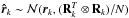 . This means that
  has a complex Gaussian distribution
  . Because astronomical sources are usually much weaker than the system noise, it is common to use the approximation Rk ≈ Rn,k. With this approximation and using the independence of system noise on each receiving element (antenna or station), we can assume that Rn,k is diagonal and that
 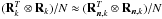 is also a diagonal approximation of the noise covariance matrix on the visibility samples. With this framework we can write the natural weighting as
 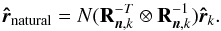 (A.2)This shows that natural weighting is a very reasonable approximation of the weighting used when solving (28)for WLS (except for a factor N that drops out from both sides).
Next, we relate WLS to Robust Weighting (Briggs 1995) by assuming slightly different simplifications. Let us assume that  and let us consider a single source with intensity σ then we have for
 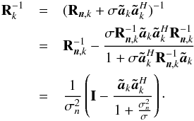 (A.3)Compared to natural weighting, now not only the noise power but also the available signal power is taken into account for the weighting. The term
  is the same as the parametric Wiener filter in the Fourier domain as given by (Briggs 1995) which relates Robust Weighting to standard signal processing concepts. However Robust Weighting also takes the visibility sampling of the gridded uv-plane into account when calculating the weights, which is not explained in the derivation above. Hence the exact relation between Robust Weighting and WLS is still missing. This relation is interesting and should be addressed in future works.
Appendix B: Using beamformers to find upper bounds
In this section we show how to use linear beamformers to define an upper bound for the image. We also show that ASSC gives the tightest bound if we use true covariance matrix R. We also show that the MVDR dirty image is an upper bound but tighter than MF dirty image.
Let us define a beamformer  , then we observe that each pixel in the MF dirty image is the output of this beamformer:
 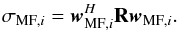 (B.1)As indicated in Sect. 3.2, we can extend this concept to a more general beamformer wi. The output power of this beamformer, in the direction of the ith pixel, becomes
  (B.2)If we require that
  (B.3)we have
 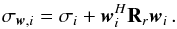 (B.4)As before, the fact that Rr is positive definite implies that
  (B.5)We can easily verify that wMF,i satisfies Eq. (B.3)and hence σMF,i is a specific upper bound. We can translate the problem of finding the tightest upper bound to the following optimization question:
 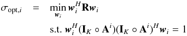 (B.6)where σopt,i would be this tightest upper bound.
To solve this optimization problem we follow standard optimization techniques and define the Lagrangian and take derivatives with respect to w and the Lagrange multiplier μ. This leads to the following system 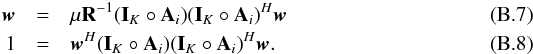 Because R is full–rank and Eq. (B.8)we can model w as
 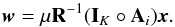 (B.9)Filling back into Eq. (B.7)we have
  (B.10)and
  (B.11)Multiplying both sides of this equation by (IK°Ai)H we get
  (B.12)Doing the same for Eq. (B.8)we have
  (B.13)Now we use Eq. (B.12)and we find
  (B.14)which makes finding x an eigenvalue problem. By taking a closer look at the matrix (IK°Ai)HR-1(IK°Ai) we find that this matrix is diagonal
 ![Mathematical equation: \appendix \setcounter{section}{2} \begin{equation} \begin{array}{l} (\bI_K \circ \bA_i)^H\bR^{-1}(\bI_K \circ \bA_i)=\\[3mm] ~~~~~~~~~\begin{bmatrix} \ba_{1,i}^H\bR_1^{-1}\ba_{1,i} & \zeros & \dots & \zeros \\ \zeros & \ba_{i,2}^H\bR_2^{-1}\ba_{i,2} &&\vdots \\ \vdots & &\ddots & \zeros\\ \zeros &\dots &\zeros & \ba_{i,K}^H\bR_K^{-1}\ba_{i,K} \end{bmatrix} \end{array} \end{equation}](/articles/aa/full_html/2016/04/aa26214-15/aa26214-15-eq410.png) (B.15)and hence x = em is an elementary vector with all entries equal to zero except for mth entry which equals unity. m is the index corresponding to largest eigenvalue, λmax, and from Eq. (B.12)we have μ = 1 /λmax. Filling back for w we find
(B.15)and hence x = em is an elementary vector with all entries equal to zero except for mth entry which equals unity. m is the index corresponding to largest eigenvalue, λmax, and from Eq. (B.12)we have μ = 1 /λmax. Filling back for w we find  (B.16)and the output of the beamformer
 ![Mathematical equation: \appendix \setcounter{section}{2} \begin{eqnarray} \sigma_{\rm opt}&=& \bw_{i,\text{opt}}^H\bR\bw_{i,\text{opt}} \notag \\[3mm] &=&\frac{\ba_{i,m}^H\bR^{-1}_m\ba_{i,m}}{(\ba_{i,m}^H\bR^{- 1}_m\ba_{i,m})^2} \notag \\[3mm] &=&\frac{1}{\ba_{i,m}^H\bR_m^{-1}\ba_{i,m}} \notag \\[3mm] &=&\min_k\left(\frac{1}{\ba_{k,i}^H\bR_k^{-1}\ba_{k,i}}\right)\cdot \end{eqnarray}](/articles/aa/full_html/2016/04/aa26214-15/aa26214-15-eq415.png) (B.17)In order to reduce the variance of this solution we suggest to find a beamformer that instead of Eq. (B.3) satisfies the slightly different normalization constraint
(B.17)In order to reduce the variance of this solution we suggest to find a beamformer that instead of Eq. (B.3) satisfies the slightly different normalization constraint  (B.18)We show that the expected value of the resulting dirty image constitutes a larger upper bound than the ASSC (40), but because the output power of this beamformer depends on more than one snapshot it has a lower variance than ASSC, so that it is more robust in practice.
With this constraint, the beamforming problem is 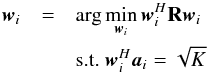 (B.19)which is recognized as the classical minimum variance distortionless response (MVDR) beamforming problem (Capon 1969). Thus, the solution is given in closed form as
  (B.20)To demonstrate that this image is still an upper bound we show that
  (B.21)Indeed, inserting (B.20)into this inequality gives
 ![Mathematical equation: \appendix \setcounter{section}{2} \begin{equation} \begin{array}{l} \label{eq:MVDRUB2} K\frac{\ba_i^H\bR^{-1}(\bI_K \circ \bA^i)(\bI_K \circ \bA^i)^H\bR^{-1}\ba_i}{(\ba_i^H\bR^{-1}\ba_i)^2} = K \frac{\sum_k (\ba_{k,i}^H\bR_k^{-1}\ba_{k,i})^2}{\left(\sum_k \ba_{k,i}^H\bR_k^{-1}\ba_{k,i}\right)^2}\\[3mm] ~~~~~~~~~~ = K\frac{\bh^T\bh}{\bh^T\ones_K\ones_K^T\bh} \geq K\frac{1}{\lambda_{\text{max}}(\ones_K\ones_K^T)}=1, \end{array} \end{equation}](/articles/aa/full_html/2016/04/aa26214-15/aa26214-15-eq420.png) (B.22)where h = (IK°Ai)HR-1ai is a K × 1 vector with entries
(B.22)where h = (IK°Ai)HR-1ai is a K × 1 vector with entries  and λmax(·) is the largest eigenvalue of of the argument matrix. Hence, a similar reasoning as in Eq. (B.2) gives
  which leads to formula (42).
Note that wMF,i also satisfies the constraint in Eq. (B.19), i.e.  , but does not necessary minimize the output power
  , therefore the MVDR dirty image is smaller than the MF dirty image: σMVDR ≤ σMF. Thus it is a tighter upper bound. This relation also holds if R is replaced by the sample covariance .
Appendix C: Variance of the dirty image
To find the confidence intervals for the dirty images we need to find estimates for the variance of both matched filter and MVDR dirty images. In our problem the sample covariance matrix is obtained by squaring samples from a Gaussian process. This means that  where
where  is the Wishart distribution function of order p with expected value equal to R and N degrees of freedom. For any deterministic vector ζ,
  (C.1)where χ2(N) is the standard χ2 distribution with N degrees of freedom. In radio astronomical applications N is usually very large and we can approximate this χ2 distribution with a Gaussian such that
  .
The variance of the matched filter dirty image is given by
.
The variance of the matched filter dirty image is given by  Using this result we can find the x% confidence interval which results in an increase of the upper bound such that
  (C.2)where α is chosen depending on x. Requiring at most a single false detection on the entire image translate into α ≈ 6.
When we estimate the MVDR dirty image from sample covariance matrices we need to be more careful, mainly because the result is biased and we need to correct for that bias. For each pixel of the MVDR dirty image obtained from sample covariance matrices we have  (C.3)where g(Z) = 1 /Z and
  . Using a perturbation model Z = Z0 + ΔZ and a Taylor approximation we find
  (C.4)Let Z0 = ℰ { Z } then ℰ { ΔZ } = 0 and ℰ { g(Z) } ≈ 1 /Z0. We would like this estimate to be unbiased which means that we want
  (C.5)however we have,
  (C.6)where we have used
  (Shaman 1980). So in order to remove this bias we need to scale it by a correction factor
  (C.7)and
  (C.8)Now we need to find an estimate for the variance of the MVDR dirty image. Using Eq. (C.4)we see that the first order approximation of
  . We find Var(Z) using the independence of each snapshot so we can write
  (C.9)In order to find
  we need to use some properties of the complex inverse Wishart distribution. A matrix has
complex inverse Wishart distribution if it’s inverse has a complex Wishart distribution (Shaman 1980). Let us define an invertible matrix B as  (C.10)then
  has an inverse Wishart distribution because
  has a Wishart distribution. In this case
  also has an inverse Wishart distribution with less degrees of freedom. The covariance of an inverse Wishart matrix is derived in (Shaman 1980), however because we are dealing only with one element, this results simplifies to
 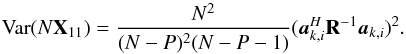 (C.11)The variance of the unbiased MVDR dirty image is thus given by
 ![Mathematical equation: \appendix \setcounter{section}{3} \begin{eqnarray} \Var(\UMVDRDIind{i})&=&\Var(C K g(Z))\notag \\[3mm] &\approx& \frac{K^2}{(N-P-1)}\frac{\sum_k (\ba_{k,i}^H\bR_{k}^{-1}\ba_{k,i})^2}{\left(\sum_k \ba_{k,i}\bR_{k}^{-1}\ba_{k,i}\right)^4}\cdot\notag \end{eqnarray}](/articles/aa/full_html/2016/04/aa26214-15/aa26214-15-eq464.png) Now that we have the variance we can use the same method that we used for MF dirty image to find α and
Now that we have the variance we can use the same method that we used for MF dirty image to find α and 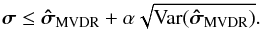 (C.12)
All Tables
All Figures
|
Fig. 1 Contoured true source on dB scale. |
| In the text | |
|
Fig. 2 Contoured dirty images on dB scale. a) MF dirty image. b) MVDR dirty image. |
| In the text | |
|
Fig. 3 Extended source simulations. Units for the first and third columns are in dB. Linear scale is used for residual images (second column). a) CLEAN Image. b) CLEAN Residual image. c) CLEAN cross-section. d) Solution of CLS + MF. e) Residual image for CLS + MF. f) Cross-section for CLS + MF. g) Solution of CLS + MVDR. h) Residual image for CLS + MVDR. i) Cross-section for CLS image + MVDR. j) CPWLS image. k) CPWLS residual image. l) MVDR dirty image and CPWLS cross-section. |
| In the text | |
|
Fig. 4 Point source simulations. a) Position estimates. b) Full sky MF dirty image in dB (with respect to 1 Jy). |
| In the text | |
|
Fig. 5 Reconstructed images in dB (with respect to 1 Jy) scale and residual images on linear scale. a) Reconstructed image with grid correction plus residual image. b) Residual image using active set and grid correction. c) Reconstructed image with CLEAN plus residual image. d) Residual image using CLEAN. |
| In the text | |
Current usage metrics show cumulative count of Article Views (full-text article views including HTML views, PDF and ePub downloads, according to the available data) and Abstracts Views on Vision4Press platform.
Data correspond to usage on the plateform after 2015. The current usage metrics is available 48-96 hours after online publication and is updated daily on week days.
Initial download of the metrics may take a while.