© ESO, 2016

1. Introduction

Starting from the seminal paper of Shakura and Sunyaev (1973), magnetic fields have been seen to play an important role in various explanations of the accretion discs physics and phenomenology. In particular, magnetic fields are central to understanding the angular momentum transport in the disc as well as the collimation by magnetic fields of jets in various accretion disc systems; see e.g. Balbus & Hawley (1991), Blandford & Znajek (1977), Blandford & Payne (1982), Stone et al. (1996), Narayan et al. (2014).

More generally, accretion discs are discussed in several branches of astronomy and the associated magnetic fields can, in principle, have various natures. Broadly speaking, magnetic fields in a disc system may be transported with the accreted matter, either being associated with the central body and/or jet, and can be fossil or dynamo excited in situ (e.g. Lubow et al. 1994; Okuzumi et al. 2014).

The important point is that a rotating accretion disc is a body which can also provide dynamo excitation. Indeed, accretion discs are thought to possess differential rotation and turbulence, i.e. two types of motions important for dynamo action. The medium of accretion discs is believed to be sufficiently conductive that induction effects dominate over dissipation. Coriolis force and density stratification affect turbulence and are assumed to make it mirror asymmetric. As a result, all the components of conventional disc dynamos that have been thoroughly investigated for the discs of spiral galaxies are also found in accretion discs, and it can be expected that magnetic field excitation of a nature quite similar to that in spiral galaxies will occur.

On the other hand, the hydrodynamics of accretion discs is obviously different in some respects from that of spiral galaxies. In particular, flat rotation curves are typical of spiral galaxies whilst a Keplerian rotation law is usually assumed for accretion discs. Moreover, substantial radial flows are thought to occur in accretion discs, whereas radial flows appear to be weak in the greater part of most spiral galaxies.

Of course, the problem has attracted the attention of dynamo theorists, and a number of papers have been focused on simulating dynamo processes in the framework of direct numerical simulations, typically in a sheared box representing a part of an accretion disc (e.g. Pariev & Colgate 2007a,b; Stone et al. 1996; Davis et al. 2010; Jiang et al. 2013). The message from these investigations is that dynamo action quite similar to that in galactic discs also occurs in accretion discs. In particular, Gressel & Pessah (2015), based on the analysis of a quite sophisticated numerical model, conclude that their findings give additional support to the importance of the αΩ-mechanism in determining the evolution of large-scale magnetic fields in turbulent accretion disks; see also Blackman (2012).

On the other hand, it is quite problematic to extrapolate a shear box simulation to a general scenario for magnetic field configurations in entire accretion discs, and to identify the link between the disc parameters and such configurations. Of course, it is very important to connect the local shear-box simulations with global disc dynamo action (e.g. Sadowski et al. 2015). However, understanding the link between the physical parameters of the disc and the dynamo driven magnetic configuration is still problem that requires clarification. Certainly, it is not clear in advance how specific the configuration of dynamo generated magnetic field in accretion discs is.

A common practice in studies of galactic discs is to consider relatively simple mean-field models as a complement to direct numerical simulations. Mean-field modelling provides an understanding of the magnetic configuration as a whole ignoring finer details. In our opinion, study of mean-field dynamo models for accretion discs can provide a valuable synergy with direct numerical simulations in shear boxes. This is the aim of the present paper. We begin by modelling the entire radial extent of the disc, with a realistic vertical thickness, for a range of dynamo parameters, using a quasi-kinematic approach (i.e. with a simple alpha-quenching non-linearity only). Then, with a slightly radially truncated model we also include a representation of the action of the Lorentz force of the large-scale field on the azimuthal velocities.

Our strategy is to consider as a basic example a standard hydrodynamical model for accretion discs of cataclysmic variables as celestial bodies which includes as few non-standard physics as possible, and to play with numbers around those of the basic model. We anticipate that this will provide hints as to what might be expected from such an approach applied to discs around black holes. We concentrate on the disc dynamo only and for the time being ignore what might happen arising from the interplay between the disc and the central body. This approach was exploited in the 1990s as being the only one then affordable (e.g. Stepinski & Levi 1990; Torkelsson & Brandenburg 1994; Reyes-Ruiz & Stepinski 1999; Rüdiger et al. 1995, among a number of others). The models studied in these papers were constrained by the facilities then readily available to have either unrealistically thick discs, constant thickness discs, or discs truncated at relatively large inner radii. (Arlt & Rüdiger 2001, among others, studied the role of magnetorotational instability – MRI – we assume that its effects are broadly speaking subsumed into our turbulence coefficients.) At that time efforts were concentrated to some extent on the computational aspects of the problem and then on the transition from mean-field models to the direct numerical simulations (DNS) that soon became feasible (e.g. Brandenburg et al. 1995). On one hand, this seminal progress in direct numerical simulations clarified the physical nature of accretion disc dynamos, but did not allow extraction of all the astronomically important results that were available from simple mean-field models as required by the wider astronomical community. In this sense our paper is a revisiting of the older approach, but can now be viewed in the light of the contemporary understanding of the relation between abilities of modern DNS to study the detailed physics and the helpful support of the more traditional tools of mean-field.

We emphasize specifically that we will only consider magnetic fields generated by the dynamo in the accretion disc itself, rather in its surroundings.

Our paper is mainly addressed to workers in the astronomical interpretation of accretion disc phenomena. Of course, experts in dynamo modelling know without specific simulations that the simplest dynamo model for a thin disc will have a steady magnetic configuration of quadrupole symmetry, concentrated near the central plane of the disc. The problem however is that this idea has not fully penetrated the observational community, and that the constraints arising need to be discussed. In particular, a naive generalization of experience from galactic dynamos to accretion discs is risky, and may be sometimes misleading because the nature of interstellar turbulence and that of turbulence in accretion discs is different. On the other hand it seems preferable to keep in mind the rich mass of experince obtained from studies of dynamos in galactic discs, supported by direct observations, rather than just to ignore it.

2. Disc model

The conventional scenario of magnetic field generation, the αΩ-dynamo, is based on the joint action of differential rotation and mirror-asymmetric turbulence. It is conventional to represent the relative importance of these effects in terms of several dimensionless numbers similar to the Reynolds number in hydrodynamics. Our first aim is to present conservative estimates for these numbers in the discs of cataclysmic variables, and then discuss more-or-less realistic scattering of numbers around this estimates.

2.1. Basic model

We consider the steady state optically thick and geometrically thin accretion α-disc (Shakura & Sunyaev 1973) of a white dwarf. The mass accretion rate Ṁ = 10¹⁷ g s^-1 was chosen as being a typical value for nova-like variables and dwarf novae during outbursts (Warner 2003). Both of these types of objects are sub-classes of cataclysmic variable stars. We note, however, that our results will not change qualitatively if we take larger values of Ṁ. We take a typical white dwarf mass M = 0.8 M_⊙ = 1.6 × 10³³ g with radius R₀ = 7 × 10⁸ cm, which follows from the universal mass-radius relation for the white dwarfs (Nauenberg 1972). The outer disc radius is taken to be R_out = 7 × 10¹⁰ cm (R_out/R₀ ≈ 10²). We assume that the central white dwarf is not (or weakly) magnetized, and so the inner radius of the disc is close to that of the radius of the central white dwarf R_in = R₀. We use R_out as a length unit, r = R/R_out so that in dimensionless units r_out = 1, r_in = 10^-2.

The disc model is essentially that of Shakura & Sunyaev (1973). One of the important problems for the accretion disc theory is a boundary condition at the inner disc radius. Standard α-disc theory (Shakura & Sunyaev 1973) for accretion discs around black holes uses as boundary condition the vanishing of the viscous stress tensor. This condition leads to formally infinite or zero values of the basic physical properties at the inner disc radius. This appears mathematically as a numerical factor $\mathit{Q}\mathrm{\left(}\mathit{r}\mathrm{\right)}\mathrm{=}\left(\mathrm{1}\mathrm{-}\sqrt{\frac{{\mathit{r}}_{\mathrm{in}}}{\mathit{r}}}\right)$ applied to various powers in the analytical solutions for the all the physical parameters. To avoid these infinities we used below a modified factor $\mathit{Q}\mathrm{\left(}\mathit{r}\mathrm{\right)}\mathrm{=}\left(\mathrm{1}\mathrm{-}\mathit{q}\sqrt{\frac{\mathrm{0.01}}{\mathit{r}}}\right)$ with q = 0.9.

In fact, the inner boundary condition problem is much more complicated for the accretion discs around white dwarfs. A boundary layer between a slowly rotating white dwarf and a fast rotating (with Keplerian angular velocity) accretion disc must exist (Pringle & Savonije 1979; Tylenda 1977; Popham & Narayan 1995; Hertfelder et al. 2013). The dynamo action in the boundary layers is a separate problem, which we neglect here, but plan to consider in future work. Here we are interested in magnetic field generation in the accretion disc itself, and the assumed approximation is enough for our aims.

The disc in the standard theory rotates with Keplerian velocity, so that $\mathit{V}\mathrm{=}\sqrt{\mathit{GM}\mathit{/}\mathit{R}}\mathit{,} \mathrm{\Omega }\mathrm{=}\sqrt{\mathit{GM}\mathit{/}{\mathit{R}}^{\mathrm{3}}}\mathit{.}$(1)Thus V = 389 r^{− 1 / 2} km s^-1, Ω = 5.56 × 10^-4r^{− 3 / 2} s^-1, and the rotation period is P = 2πΩ^-1 = 11 298 r^{3 / 2} s. It is worth noting that Eq. (1) is quite different to the typical rotation curves of spiral galaxies: the latter have almost flat V(r), presumably because of the presence of dark matter halos around galactic discs.

To calculate all physical properties in the disc model described below we used the analytical solutions obtained by Suleimanov et al. (2007) on the basis of the Shakura & Sunyaev (1973) model, but with the appropriate opacity for the solar mix plasma and the correct vertical disc structure. The solutions derived for the gas pressure and the absorption opacity dominated accretion discs are valid for our disc model. We used a theoretical turbulent viscosity parameter α_SS = 0.1. The radial distributions of our mid-plane temperatures and density are $\mathit{T}\mathrm{=}\mathrm{1.51}\mathrm{\times }{\mathrm{10}}^{\mathrm{4}}\hspace{0.17em}{\mathit{r}}^{\mathrm{-}\mathrm{3}\mathit{/}\mathrm{4}}\hspace{0.17em}\mathit{Q}\mathrm{(}\mathit{r}{\mathrm{)}}^{\mathrm{3}\mathit{/}\mathrm{10}}\hspace{0.17em}\hspace{0.17em}\mathrm{K}\mathit{,}$(2)and $\mathit{\rho }\mathrm{=}\mathrm{7.03}\mathrm{\times }{\mathrm{10}}^{-9}\hspace{0.17em}{\mathit{r}}^{\mathrm{-}\mathrm{15}\mathit{/}\mathrm{8}}\hspace{0.17em}\mathit{Q}\mathrm{(}\mathit{r}{\mathrm{)}}^{\mathrm{11}\mathit{/}\mathrm{20}}\hspace{0.17em}\hspace{0.17em}\mathrm{g}\hspace{0.17em}\mathrm{c}{\mathrm{m}}^{-3}\mathit{.}$(3)A basic parameter for the mean-field magnetic dynamo model is a turbulent diffusivity η = lV_t/ 3, where l is a typical turbulence correlation length, and V_t is an rms value of the turbulent velocities. Formally, we have to consider η values that are consistent with the assumed α_SS, but taking into account that the above estimate is certainly over simplistic we consider it as a free parameter in order to investigate various regimes of magnetic dynamo action the accretion disc.

Accretion discs are assumed to be turbulent, and a naive estimate for the rms value of the turbulent velocities V_t is that it is a fraction of the sound speed, V_s, V_t = σ_vV_s, σ_v ≤ 1. For the basic model we assume σ_v = 1. Therefore, the turbulent diffusivity is estimated by $\mathit{\eta }\mathrm{=}\frac{\mathit{l}{\mathit{V}}_{\mathrm{t}}}{\mathrm{3}}\mathrm{=}{\mathit{\sigma }}_{\mathrm{l}}\hspace{0.17em}{\mathit{\sigma }}_{\mathrm{v}}\hspace{0.17em}\frac{\mathit{H}{\mathit{V}}_{\mathrm{s}}}{\mathrm{3}}\mathrm{·}$(4)In our approach the sound speed can be evaluated as ${\mathit{V}}_{\mathrm{s}}\mathrm{=}{\left(\frac{{\mathit{k}}_{\mathrm{B}}\mathit{T}\mathrm{\left(}\mathit{r}\mathrm{\right)}}{\mathit{\mu }{\mathit{m}}_{\mathrm{H}}}\right)}^{\mathrm{1}\mathit{/}\mathrm{2}}\mathrm{=}\mathrm{14.2}\hspace{0.17em}{\mathit{r}}^{\mathrm{-}\mathrm{3}\mathit{/}\mathrm{8}}\mathit{Q}\mathrm{(}\mathit{r}{\mathrm{)}}^{\mathrm{3}\mathit{/}\mathrm{20}}\hspace{0.17em}{\mathrm{km}\hspace{0.17em}\mathrm{s}}^{-1}\mathit{.}$(5)Thus V_s has a maximum of 53 km s^-1 at r = 1.36 r_in and smoothly decreases to V_s = 14 km s^-1 at r = 1.

Usually it is assumed that l is close to, although somewhat smaller than, the disc scale height H. To be specific we use l = σ_lH. For the basic model we assume σ_l = 0.2. Fortunately, results do not depend crucially on this estimate.We take the disc scale height H as an initial estimate for the disc thickness $\mathit{H}\mathrm{=}{\mathit{V}}_{\mathrm{s}}\mathit{/}\mathrm{\Omega }\mathrm{=}\mathrm{2.55}\mathrm{\times }{\mathrm{10}}^{\mathrm{9}}\hspace{0.17em}{\mathit{r}}^{\mathrm{9}\mathit{/}\mathrm{8}}\mathit{Q}\mathrm{(}\mathit{r}{\mathrm{)}}^{\mathrm{3}\mathit{/}\mathrm{20}}\hspace{0.17em}\mathrm{cm}\mathit{.}$(6)Thus the local aspect ratio is H/R ≈ 10^-2$\mathit{\lambda }\mathrm{\left(}\mathit{r}\mathrm{\right)}\mathrm{=}\frac{\mathit{H}}{\mathit{R}}\mathrm{=}\mathrm{0.037}\hspace{0.17em}{\mathit{r}}^{\mathrm{1}\mathit{/}\mathrm{8}}\hspace{0.17em}\mathit{Q}\mathrm{(}\mathit{r}{\mathrm{)}}^{\mathrm{3}\mathit{/}\mathrm{20}}\mathit{.}$(7)The infall radial velocity of matter in the disc is ${\mathit{V}}_{\mathrm{in}}\mathrm{=}\mathit{Ṁ}\mathit{/}\mathrm{(}\mathrm{2}\mathit{\pi R}\hspace{0.17em}\mathit{H\rho }\mathrm{)}\mathrm{=}\mathrm{0.13}\hspace{0.17em}{\mathit{r}}^{\mathrm{-}\mathrm{1}\mathit{/}\mathrm{4}}\hspace{0.17em}\mathit{Q}\mathrm{(}\mathit{r}{\mathrm{)}}^{\mathrm{-}\mathrm{7}\mathit{/}\mathrm{10}}\hspace{0.17em}\hspace{0.17em}\mathrm{km}\hspace{0.17em}{\mathrm{s}}^{-1}\mathit{.}$(8)Another important physical parameter is the equipartition magnetic field strength, which can be estimated by assuming that the magnetic pressure is in equilibrium with the energy of the turbulent gas motions ${\mathit{B}}_{\mathrm{eq}}\mathrm{=}{\mathit{\sigma }}_{\mathrm{v}}{\mathit{V}}_{\mathrm{s}}\sqrt{\mathrm{4}\mathit{\pi }\hspace{0.17em}\mathit{\rho }}\mathrm{=}\mathrm{420}\hspace{0.17em}{\mathit{\sigma }}_{\mathrm{v}}\hspace{0.17em}{\mathit{r}}^{\mathrm{-}\mathrm{21}\mathit{/}\mathrm{16}}\hspace{0.17em}\mathit{Q}\mathrm{(}\mathit{r}{\mathrm{)}}^{\mathrm{17}\mathit{/}\mathrm{40}}\hspace{0.17em}\hspace{0.17em}\mathrm{G}\mathit{.}$(9)Excitation of mean field disc dynamos is usually assumed to be by the α Ω mechanism, based on the joint action of differential rotation Ω(r) and the mirror asymmetric (from the action of the Coriolis force) turbulence: α is a measure of this asymmetry and has dimensions of velocity. Conventionally $\mathit{\alpha }\mathrm{=}{\mathit{l}}^{\mathrm{2}}\hspace{0.17em}\frac{\mathrm{\Omega }}{\mathit{H}}\mathrm{=}{\mathit{\sigma }}_{\mathrm{l}}^{\mathrm{2}}\hspace{0.17em}\mathit{V}s$(10)in z> 0 (and is antisymmetric w.r.t. z).

Now we can define dimensionless measures of the contributions to dynamo action of each from the principal drivers. Thus ${\mathit{R}}_{\mathit{\omega }}\mathrm{=}\frac{{\mathit{H}}^{\mathrm{2}}\mathrm{\Omega }}{\mathit{\eta }}\mathrm{=}{\mathit{V}}_{\mathrm{s}}\frac{\mathit{H}}{\mathit{\eta }}\mathrm{=}\frac{\mathrm{3}}{{\mathit{\sigma }}_{\mathrm{l}}{\mathit{\sigma }}_{\mathrm{v}}}\mathit{,}$(11)and ${\mathit{R}}_{\mathit{\alpha }}\mathrm{=}\mathit{\alpha }\hspace{0.17em}\frac{\mathit{H}}{\mathit{\eta }}\mathrm{=}{\mathit{R}}_{\mathit{\omega }}\hspace{0.17em}\frac{\mathit{\alpha }}{{\mathit{V}}_{\mathrm{s}}}\mathrm{=}\mathrm{3}\frac{{\mathit{\sigma }}_{\mathrm{l}}}{{\mathit{\sigma }}_{\mathrm{v}}}\mathit{,}$(12)where Eqs. (4) and (10) were used. These determinations of R_ω and R_α give a local dynamo number $\mathit{D}\mathrm{\left(}\mathit{r}\mathrm{\right)}\mathrm{=}{\mathit{R}}_{\mathit{\alpha }}{\mathit{R}}_{\mathit{\omega }}\mathrm{=}\frac{{\mathit{H}}^{\mathrm{3}}\mathit{\alpha }\hspace{0.17em}\mathrm{\Omega }}{{\mathit{\eta }}^{\mathrm{2}}}\mathrm{=}\mathit{\alpha }\hspace{0.17em}{\mathit{V}}_{\mathrm{s}}\frac{{\mathit{H}}^{\mathrm{2}}}{{\mathit{\eta }}^{\mathrm{2}}}\mathrm{=}\mathrm{9}\hspace{0.17em}{\mathit{\sigma }}_{\mathrm{v}}^{-2}\mathit{.}$(13)Remarkably, D(r) is independent of radius if we assume that σ_v is a constant over the disc. (The numerical factor 3 in Eq. (4) comes from the dimension of the space.) There is also a subsidiary parameter, a Reynolds number ${\mathit{R}}_{\mathrm{m}}\mathrm{=}{\mathit{V}}_{\mathrm{in}\mathit{,}\mathrm{0}}\frac{{\mathit{H}}_{\mathrm{0}}}{{\mathit{\eta }}_{\mathrm{0}}}\mathrm{=}{\mathit{R}}_{\mathit{\omega }}\hspace{0.17em}\frac{{\mathit{V}}_{\mathrm{in}\mathit{,}\mathrm{0}}}{{\mathit{V}}_{\mathrm{s}\mathit{,}\mathrm{0}}}\mathrm{\approx }\mathrm{0.14}\left(\frac{\mathrm{0.2}}{{\mathit{\sigma }}_{\mathrm{v}}{\mathit{\sigma }}_{\mathrm{l}}}\right)\mathit{,}$(14)which is found to play a minor role.

The above estimate of dynamo number D is well-known in dynamo theory, and discussed by Stepinski & Levi (1990). Our aim here is to emphasize the constraints that follow from this estimate in simple dynamo models, as well as ways of proceeding further. In particular, already Rüdiger et al. (1995) mentioned that the estimate only determines properties of 1D disc models, and that 2D models need separate, more detailed, consideration.

It is also useful to define a magnetic diffusive time scale for the disc model $\mathit{\tau }\mathrm{=}\frac{{\mathit{H}}^{\mathrm{2}}}{\mathit{\eta }}\mathrm{=}{\mathit{R}}_{\mathit{\omega }}\hspace{0.17em}\frac{\mathit{H}}{{\mathit{V}}_{\mathrm{s}}}\mathrm{=}\frac{\mathrm{3}}{{\mathit{\sigma }}_{\mathrm{l}}\hspace{0.17em}{\mathit{\sigma }}_{\mathrm{v}}}{\mathrm{\Omega }}^{-1}\mathrm{\approx }\mathrm{27}\hspace{0.17em}\mathrm{780}\hspace{0.17em}\left(\frac{\mathrm{0.2}}{{\mathit{\sigma }}_{\mathrm{l}}\hspace{0.17em}{\mathit{\sigma }}_{\mathrm{v}}}\right)\hspace{0.17em}{\mathit{r}}^{\mathrm{3}\mathit{/}\mathrm{2}}\hspace{0.17em}\mathrm{s}\mathit{.}$(15)For comparison, the dynamo number in the discs of spiral galaxies is also estimated to be about D = 9, and there results in excitation of large-scale magnetic fields of quadrupole symmetry that are almost totally confined to the disc. According to experience from discs of spiral galaxies, generation of magnetic fields of dipole symmetry in the space surrounding the disc requires D> 100 at least. Just for orientation, D = 10³ ~ 10⁵ in the spherical shell inside the Sun where dynamo action resulting in generation of the solar dipole magnetic field is thought to occur.

Of course, the above estimates provides a hint only and specific modelling of dynamo action in accretion discs is essential. However we can conclude that the scaling of Eq. (13) plays a crucial role in the problem. The underlying physics for the Eq. (13) is the identification of the turbulent velocities of the accretion disc medium and the sound speed, which in turn determines the pressure height scale of the disc H.

2.2. Parameter space near the basic model

Given that our basic model certainly does not reproduce accurately and in detail the properties of real accretion discs, we need to consider plausible modifications of the model and thus of the estimate (13). Our “standard” case (above) has σ_v = 1,σ_l = 0.2. Inter alia, we can adjust the relative roles of differential rotation and mirror asymmetric turbulence rescaling σ_v and σ_l while keeping D constant.

Using the above scaling we can obtain the dynamo number D ≫ 9, i.e. if the turbulent velocities are substantially lower then the sound speed (σ_v ≪ 1). Therefore, the dynamo number can be substantially larger than that in the basic model and the variety of dynamo driven magnetic configuration may become richer. More specifically, we need σ_v = 0.1 ~ 0.3 to expect something more than the quadrupolar field excitation that is well-known from galactic dynamo studies. Below (Sect. 4.4) we face one more problem with definition of dynamo governing parameters: when developing our model from 1D to 2D we have to modify the definitions of R_α, R_ω and R_m. This can be done by a multiplier which formally plays the same role as σ_v however its physical meaning is different. In order to emphasize this point we introduce a quantity f_v multiplying each of R_α,R_ω and R_m simultaneously. This allows a systematic exploration of parameter space. From a dynamo theory viewpoint, it is natural to test the sensitivity of the model to changes in dynamo number including the cases f_v< 1 as well as f_v> 1 while σ_v> 1 (f_v< 1) formally corresponds to supersonic turbulence which taken literally would not be realistic. In the restricted context of dynamo theory this restriction does not apply, and in any case it would be rash to assume that our model for the disc can be interpreted too exactly.

Dynamo action for a given flow gives an exponentially growing magnetic field which quite rapidly becomes strong enough to affect the fluid motions, resulting in dynamo saturation and formation of the eventual magnetic configuration. The particular form of the saturation is still a disputed topic. However experience of galactic dynamos (see e.g. Kleeorin et al. 2000, 2002, 2003 where a sequence of more and more complicated models of dynamo saturation is used, giving very similar saturated magnetic field configurations as in the simplest case) suggests that a reasonable approximation to the final configuration can be obtained using a simple expression of the form $\mathit{\alpha }\mathrm{=}\frac{{\mathit{\alpha }}_{\mathrm{0}}}{\mathrm{1}\mathrm{+}\mathit{\xi }{\mathit{B}}^{\mathrm{2}}\mathit{/}{\mathit{B}}_{\mathrm{eq}}^{\mathrm{2}}}\mathit{,}$(16)where α₀ is the unsaturated value and ξ is a numerical factor of order unity. Below we use this approach taking ξ = 1 and bearing in mind the approximate nature of the approach. Note that changing the value of ξ merely rescales magnetic field in the saturated solutions.

3. Alpha-quenched model

3.1. Preliminaries

Following the idea of our paper, we are interested in relatively simple models for dynamo driven magnetic configurations. Experience from models for galactic dynamos suggests that a substantial simplification of the general mean-field dynamo equations is also possible for accretion discs. Indeed, for the basic model, we expect excitation of a solution symmetric with respect to the disc equatorial plane, i.e. a configuration with quadrupole symmetry. Galactic dynamo studies suggest a method to reduce the mean-field equations for such a configuration to relatively simple forms, which give mean or integral values taken perpendicular to the disc of magnetic field components parallel to the disc (this is known as the no-z approximation: Subramanian & Mestel 1993; Moss 1995). On the other hand, the dynamo drivers have axisymmetric distributions and it looks plausible that the dynamo driven magnetic may also be axisymmetric.

We start our analysis from some trial solutions constructed using this approximation. Solutions were found assuming axisymmetry (i.e. a 1D problem. The marginal case occurs for σ_v ~ 1.54, i.e. D ~ 3.8. Then a φ-dependent case in 2D was run (where φ is the azimuthal coordinate). Although the latter solutions were not followed to saturation, there was a very strong indication that saturated solutions would be axisymmetric (in accordance with naive expectations). Thus, through the remainder of this paper axisymmetry is assumed. However, we cannot exclude the possibility that for very supercritical solutions axisymmetry may be lost.

3.2. Basic 1D model

The inner computational boundary is placed at the inner disc boundary r = r_in = 0.01. We use 4001 uniformly spaced grid points which seems to be more than sufficient. For this approximation, the inner boundary condition is rather arbitrary, and we simply extrapolate B_r from the next two points, and determine B_φ(in) by requiring the ratio ${\mathit{B}}^{\mathrm{2}}\mathrm{\left(}\mathrm{in}\mathrm{\right)}\mathit{/}{\mathit{B}}_{\mathrm{eq}}^{\mathrm{2}}\mathrm{\left(}\mathrm{in}\mathrm{\right)}$ to have the same value as at the next point (the global solution is rather insensitive to this b.c.).

Fig. 1 Global solution (left) and a magnified view of the solution near r = rin (right), for the slightly supercritical parameters Rα = 0.6, Rω = 15, Rm = 0.146. In upper panels solid line is for Beq and dashed line stands for Bφ.

The final (saturated) magnetic configuration is shown in Fig. 1 for the basic model. We can experiment with the model, keeping the main parameter D constant.

The steep rise in field towards r = r_in appears robust (e.g. to change of b.c., and to extension of the computational domain to r<r_in as well as to enlargement of the infall velocity). Typically, B_φ exceeds very slightly the equipartition value throughout the disc. The solution is rather “lat” w.r.t. r over most of the range, presumably a consequence partly at least of the constant local dynamo number and the relatively small dependence of B_eq on r in the outer regions of the disc.

We then experimented with enhancing the infall speed in the inner part of the disc, to simulate the fall of material onto the central object. For example, we enhance the radial velocity in the innermost disc by putting u_{r ∗}(r) = u_r(r) ∗ (0.10 /r)⁴ in r< 0.10, where u_r(r) is that given by the standard solution, and u_{r ∗}(r) is the velocity used. There are just modest changes to the inner solution. In particular the local maxima of B_r,B_φ are removed. This suggests that very strong enhancements to u_r are required for significant changes.

4. The 2D solutions

Of course, the above 1D approach gives only some preliminary orientation, and its extension to two dimensions seems natural. In particular, it enables consideration of magnetic configurations that are not symmetric with respect to the disc plane (i.e. not quadrupole-like) and in particular mixed parity solutions become accessible. Also the z-dependence of the dynamo driven magnetic field can be described.

4.1. Extension of the disc model to two dimensions

The canonical accretion disc model described in Sect. 2.1 has no z-dependence. To generate a model suitable for studying (axisymmetric) dynamo action in two spatial dimensions the basic model must be extended (necessarily in a rather arbitrary fashion) to depend on the vertical coordinate z. In the following the subscript d refers to values in the 1D model of Sect. 2.1. η_m is defined to be the asymptotic value of the turbulent diffusivity η far from the disc. This is a commonly made assumption in embedded disc models for galaxies, and is made to approximate a vacuum field at large distances. Taking into account that vacuum formally corresponds to infinite η we assume that η_m ≫ η_d. This important point is discussed in a galactic context by Sokoloff & Shukurov (1990): however other opinions have been presented in the literature. Rather arbitrarily we take η_m = 5η_d.

The α coefficient is written as $\begin{array}{ccc}\mathit{\alpha }\mathrm{\left(}\mathit{r,z}\mathrm{\right)}& \mathrm{=}& {\mathit{\alpha }}_{\mathrm{d}}\mathit{,}\mathrm{\left|}\mathit{z}\mathrm{\right|}\mathrm{\le }{\mathit{h}}_{\mathrm{d}}\mathrm{\left(}\mathit{r}\mathrm{\right)}\mathrm{;}\\ \mathit{\alpha }\mathrm{\left(}\mathit{r,z}\mathrm{\right)}& \mathrm{=}& \end{array}$Similarly $\begin{array}{ccc}\mathit{\eta }\mathrm{\left(}\mathit{r,z}\mathrm{\right)}& \mathrm{=}& {\mathit{\eta }}_{\mathrm{d}}\mathrm{\left(}\mathit{r}\mathrm{\right)}\mathit{,}\mathrm{\left|}\mathit{z}\mathrm{\right|}\mathrm{\le }\mathrm{2.5}{\mathit{h}}_{\mathrm{d}}\mathrm{\left(}\mathit{r}\mathrm{\right)}\mathrm{;}\\ \mathit{\eta }\mathrm{\left(}\mathit{r,z}\mathrm{\right)}& \mathrm{=}& {\mathit{\eta }}_{\mathrm{d}}\mathrm{\left(}\mathit{r}\mathrm{\right)}\mathrm{(}{\mathit{\eta }}_{\mathrm{m}}\mathrm{-}{\mathit{\eta }}_{\mathrm{d}}\mathrm{(}\left(\mathit{r}\mathrm{\left)}\tanh \mathrm{\right(}\mathrm{\left|}\mathit{z}\mathrm{\right|}\mathrm{-}\mathrm{2.5}{\mathit{h}}_{\mathrm{d}}\mathrm{\left(}\mathit{r}\mathrm{\right)}\right)\mathit{,}\\ & & \mathrm{\left|}\mathit{z}\mathrm{\right|}\mathit{>}\mathrm{2.5}{\mathit{h}}_{\mathrm{d}}\mathrm{\left(}\mathit{r}\mathrm{\right)}\mathit{.}\\ {\mathit{u}}_{\mathrm{r}}\mathrm{\left(}\mathit{r,z}\mathrm{\right)}& \mathrm{=}& {\mathit{V}}_{\mathrm{in}}\mathrm{\left(}\mathit{r}\mathrm{\right)}\mathit{,}\mathrm{\left|}\mathit{z}\mathrm{\right|}\mathrm{\le }{\mathit{h}}_{\mathrm{d}}\mathrm{\left(}\mathit{r}\mathrm{\right)}\mathrm{;}\\ {\mathit{u}}_{\mathrm{r}}\mathrm{\left(}\mathit{r,z}\mathrm{\right)}& \mathrm{=}& {\mathit{V}}_{\mathrm{in}}\mathrm{\left(}\mathit{r}\mathrm{\right)}\exp \left(\mathrm{-}\frac{\mathrm{\left|}\mathit{z}\mathrm{\right|}\mathrm{-}{\mathit{h}}_{\mathrm{d}}\mathrm{\left(}\mathit{r}\mathrm{\right)}}{\mathrm{2.5}{\mathit{h}}_{\mathrm{d}}\mathrm{\left(}\mathit{r}\mathrm{\right)}}\right)\mathit{,}\mathrm{\left|}\mathit{z}\mathrm{\right|}\mathit{>}\mathrm{2.5}{\mathit{h}}_{\mathrm{d}}\mathrm{\left(}\mathit{r}\mathrm{\right)}\mathit{.}\end{array}$For the bulk of the computations Ω(r,z) = Ω_d(r). In two trial cases Ω(r,z) decreased with distance from the disc plane in a rather arbitrary manner – see Sect. 4.5. Subscript d denotes a property of the 1D disc model.

Fig. 2 Global solution (left, contours of the poloidal field) and a magnified view of the solution near r = rin (right, contours of toroidal field), for the somewhat supercritical parameters in the 2D model (fv = 0.3). Even parity, P = + 1. In this and subsequent figures, contours are equally spaced, solid contours correspond to positive values, broken contours represent negative values, and the dashed curve shows the disc boundary. In the right hand panel the maximum toroidal field strength occurs at r ≈ 0.015,z = 0 and is approximately 4 × 105 G. The contour interval is approximately 8 × 104 G. In all the models the poloidal field is weaker: here the mean global ratio of poloidal to toroidal field strengths is about 10-2. In this and subsequent figures, the field strength beyond the outermost contour is smaller than that at the outermost contour.

4.2. Code

The code used was written in cylindrical (r,z) geometry, based loosely on that of Moss & Shukurov (2004). Given the assumed axisymmetry, the poloidal component of the magnetic field can be written as B_pol = ∇ × A_φ, where φ is the azimuthal coordinate, and the problem then reduces to solving the evolution equations for A_φ and B_φ. The principle numerical difficulties to be overcome are the extremely small disc thickness near the inner boundary at r = r_in = 0.01 and the strong gradient of angular velocity near this inner boundary. The second difficulty was addressed quite satisfactorily by using log r as the radial coordinate, with n_r = 151 or 301 points distributed uniformly between log (r_in) and log (1). The computational domain included the disc plane z = 0, and computations were performed either in 0 ≤ z ≤ z_m, or in −z_m ≤ z ≤ z_m. This made using a logarithmic vertical coordinate problematic, and it was decided to use the “brute force” method of taking a closely spaced, uniform, vertical grid with n_z large enough to resolve satisfactorily the inner regions of the disc. With z_m = 0.2, taking n_z = 8001 was found to be adequate for calculations over the half-range, and n_z = 16 001 for the full range. Trial integrations for a supercritical case with f_v = 1 (Sect. 4.5) in the half-space z ≥ 0 confirmed that doubling the radial resolution to n_r = 301 grid points, or increasing n_z to 16 001, did not significantly affect the results.

The small spatial steps mean that a Runga-Kutte type code was not viable, as it would require extremely small time steps. Thus, as in Moss & Shukurov (2004) a Dufort-Frankel integrator was used; Δτ = 5 × 10^-5 was found to be satisfactory.

4.3. Boundary conditions

Boundary conditions are again necessarily somewhat arbitrary, but are chosen partly in the light of what previous experience has shown to be plausible and to give physically realistic results.

On the upper and lower boundaries z = ± z_m, $\begin{array}{ccc}\frac{\mathit{\partial }{\mathit{A}}_{\mathit{\phi }}}{\mathit{\partial z}}\mathrm{=}\frac{\mathit{\partial }{\mathit{B}}_{\mathit{\phi }}}{\mathit{\partial z}}\mathrm{=}\mathrm{0.}& & \end{array}$When the equations are solved in the half space $\mathrm{0}\mathrm{\le }\mathit{z}\mathrm{\le }{\mathit{z}}_{}$ the boundary conditions on z = 0 are determined by the imposed symmetry. On r = 1, $\begin{array}{ccc}\frac{\mathit{\partial }{\mathit{A}}_{\mathit{\phi }}}{\mathit{\partial r}}\mathrm{=}\frac{\mathit{\partial }{\mathit{B}}_{\mathit{\phi }}}{\mathit{\partial r}}\mathrm{=}\mathrm{0.}& & \end{array}$On r = r_in, $\begin{array}{ccc}{\mathit{A}}_{\mathit{\phi }}\mathrm{=}{\mathit{B}}_{\mathit{\phi }}\mathrm{=}\mathrm{0}\mathit{,}& & \end{array}$so that B_r = 0 there. In practice, the solutions show that field is very small at the boundaries z = ± z_m and r = 1 so the exact boundary conditions might be expected to have little effect on the solution.

To verify this, an alternative condition of extrapolating A_φ at r = r_in from the values at the next two radial points, and requiring that the ratio | B_φ | /B_eq at r = r_in be equal to that at the next radial point, was used in one case. Except very near r = r_in, there was little change in the solution.

4.4. Procedure

If we try to compare 1D and 2D solutions, some tuning of the dynamo numbers is needed. Essentially this is because of the (rather arbitrary) extension of the 1D disc model into the vertical direction; the input of the 1D model here is via the disc half-thickness H, and exact comparison of the models is impossible. See also Rüdiger et al. (1995). We want freely to explore parameter space, initially to find models near the excitation threshold and then more generally, and so again use the numerical parameter f_v multiplying R_α,R_ω and R_m introduced previously. f_v is related to ${\mathit{\sigma }}_{\mathit{v}}^{-1}$ (Sect. 2.1); we retain the notation f_v with ${\mathit{f}}_{\mathrm{v}}\mathrm{=}{\mathit{\sigma }}_{\mathit{v}}^{-1}$ to emphasize that we deal here with a more detailed model. Note again that f_v multiplies each of the dynamo numbers. We still consider R_α = 0.6,R_ω = 15, R_m = 0.1254 to be canonical values (i.e. f_v = 1). We note again that f_v< 1 corresponds formally in our model to the physically unrealistic case of supersonic turbulence. However, as discussed earlier, we think it useful to explore such cases.

Based on the usual explanation of the α-effect as being related to the mirror asymmetry of turbulence caused by the Coriolis force in a stratified medium, we expect that R_α> 0. However taking into account the uncertainties intrinsic to the physics, solutions with negative values of the dynamo number R_α are also discussed.

4.5. R ${\mathit{\alpha }}_{}\mathit{>}\mathrm{0}$

For the basic model we found that f_v = 0.3 gives a solution somewhat above the excitation threshold. This solution (Fig. 2) is steady, symmetric with respect to the central plane of the disc (i.e. of quadrupolar symmetry) and generally resembles the corresponding solution in the 1D model. The radial extent of this solution is about [ r ] = 0.05, the maximum value of | B_φ | is below the equipartition value, (| B_φ | /B_eq ≲ 0.4, and | B_φ/B_r | ≫ 1 (the ratio of global poloidal to toroidal field energies ~10^-4).

For more supercritical parameters such a steady homogeneous state may be unstable, and indeed the temporal behaviour of saturated magnetic configurations becomes more complicated as dynamo action becomes stronger. With f_v = 1, the solution saturates with irregular temporal oscillations in the total magnetic energy integrated over the computational space – see Fig. 3. The oscillations are approximately vacillatory, with no significant migration. The magnetic field is strongly concentrated to the disc plane in the inner disc, the toroidal field more so than the poloidal. Figure 4 shows the contours of toroidal field and the poloidal field lines. The maximum local ratio of field energy to equipartition energy is approximately 0.6. The lower panel of Fig. 4 shows the contours of the ratio | B_φ | /B_eq. If the computation is begun with a seed field of odd parity and f_v = 1, there is no dynamo action and the field rapidly decays. We define parity conventionally as P = (E_even − E_odd) / (E_even + E_odd), where E_odd is the energy of the part of the field that is even with respect to the central plane of the disc, and E_odd is energy of the odd part (more details are given in the Appendix).

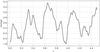Fig. 3 Temporal behaviour of the total global magnetic energy for Rα = 0.6, fv = 1. Even parity, P = + 1. (Energy is normalized with the equipartition energy at the outer radius – see Eq. (9).) Energy here and below is calculated by integration over the whole entire computaional volume (see Appendix for details).

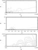Fig. 4 Solution with Rα> 0,fv = 1, even parity P = + 1. The contours lines of Bφ near the inner boundary (top panel), the poloidal field lines in the complete computational space (middle) and contours of the ratio | Bφ | /Beq (bottom). In the top panel the maximum of the toroidal field strength is about 2.4 × 105 G, and the contour spacing is approximately 4 × 104 G. In the lower panel the maximum of | B | /Beq is about 0.6 at r ≈ 0.15,z = 0, with contour spacing 0.12. In this and subsequent figures, contours are equally spaced.

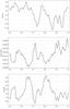Fig. 5 Temporal behaviour of the total global magnetic energy for fv = 2; solution with free parity. The upper panel shows the evolution of the parity P, the middle panel the ratio of poloidal to toroidal energies, and the lower panel the evolution of the total magnetic energy.

Given that f_v = 0.3 corresponds approximately to slightly supercritical excitation in this 2D case, this corresponds to D ~ 1 in the 1D model (see Sect. 2.1). This can be compared with the value D ≲ 4 of Sect. 3.1. There is a clear distinction between accretion disc dynamos and galactic dynamos, that is related presumably to the differing rotation curves, and maybe also to the disc geometry. There is also a divergence between the 1D and 2D solutions; as the dynamo number increases, cell structures are present in the 2D case, but not in the 1D. We speculate that these differences may have a number of causes. For example, the rotation law is Keplerian vs. more-or-less flat for galaxies. Secondly, there is now significant 2D structure in the model, and in the more supercritical cases the z-scale in the disc may impose a similar horizontal scale (somewhat analogous to the cell structure seen in some spherical thin shell dynamo models, e.g. Moss & Tuominen 1990). It remains somewhat unexpected that the no-z approximation seems to break down for these more supercritical cases. We can speculate that this is because previous comparisons of the no-z approximation with other models have been made in galactic contexts, and for the slightly supercritical cases thought to be relevant for galaxies (e.g. Phillips 2000; Chamandy et al. 2014).

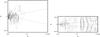Fig. 6 2D solution with free parity and Rα> 0,fv = 2; the computation extends over −zm ≤ z ≤ zm. The contour lines of Bφ near the inner boundary (left) and poloidal field lines (right) in the complete computational space.

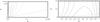Fig. 7 Solution with Rα< 0,fv = 0.25, odd parity P = −1. The contour lines of Bφ near the inner boundary (left) and the poloidal field lines in the complete computational space (right). The maximum value of | Bφ | is approximately 7.2 × 105 G, and the contour spacing is 1.2 × 105 G. The mean global ratio of poloidal to toroidal field strength is about 3 × 10-3.

Some computations were performed over the full space −z_m ≤ z ≤ z_m. We confirmed that with f_v = 1, the solution discussed above is recovered. For stronger excitation, the symmetry with respect to the disc plane is lost. The temporal behaviour and spatial structure of the solution with f_v = 2 i.e. D ≈ 36 in the 1D case) is shown in Figs. 5 and 6 respectively.

In this case, the magnetic configuration has acquired some of the characteristics of a symmetric dipole-like configuration. The toroidal magnetic field becomes concentrated near to the upper and lower boundaries of the accretion disc, instead of near the central plane as found for configurations with pure quadrupolar symmetry. The radial magnetic field profile seems to be shifted more towards the inner boundary than previously.

In two cases with f_v = 1, Ω was allowed to vary with z. In the more extreme, Ω was independent of z in 0 ≤ z ≤ h(r), and decreased with a scale height of 2.5h(r) in z>h. The global energy of the solution was significantly increased (presumably due to the increased dynamo efficiency caused by the steep gradient of Ω in the z-direction), and there was a little more radial structure. However the irregular temporal oscillations, and the general form of the solution, were very similar to those with Ω independent of z. In the other case, Ω was independent of z in 0 ≤ z ≤ 0.1, and then declined in z> 0.1. Perhaps unsurprisingly, this modification did not affect the solution strongly.

4.6. R ${\mathit{\alpha }}_{}\mathit{<}\mathrm{0}$

Taking reference values as R_α = −0.6, R_ω and R_α as above, then with f_v = 0.25 a finite amplitude odd parity solution is found. The total energy approaches its steady asymptotic value smoothly. The field structure is given in Fig. 7. Remarkably, the toroidal magnetic field is now concentrated above and below the disc rather than near the disc boundary. In our units scaled to approximately 400 G, the maximum value of B_φ is about 1500 whereas the poloidal field is very much weaker (the global ration of poloidal to toroidal field energies is about 10^-5).

5. Models with Lorentz force

The strong fields found in the innermost disc suggest that the Lorentz force may affect the rotation curve, with consequent effects on the dynamo action. Thus we amended the code to include a representation of the Lorentz force from the large-scale magnetic field on the azimuthal motions.

5.1. Amended model

Following Moss & Brooke (2000) we write $\mathit{\partial }{\mathit{v}}^{\mathrm{\prime }}\mathit{/}\mathit{\partial t}\mathrm{=}\frac{\mathrm{\nabla }\mathrm{\times }{B}\mathrm{\times }{B}}{\mathit{\rho r}}\mathrm{·}\mathit{\phi ̂}\mathrm{+}\mathrm{viscous}\mathrm{diffusion}\mathit{,}$(23)where v′ is the perturbation to the azimuthal velocity. Some smaller terms involving advection of angular momentum by the accretion velocity have been omitted. We ignore the effect of the radial component of the Lorentz force; Rekowski et al. (2000) found it to be small, albeit in a disc model that did not extend to the small fractional radii considered here. Note that the alpha-quenching non-linearity is also retained in the modelling. In this part of the investigation we amended the basic rotation curve within radius 0.03, from the Keplerian law to a linear law – see the broken curves in Fig. 8. The immediate motivation for this softening of Ω is to avoid computation difficulties, and to allow some progress to be made. With too rapid inward growth of angular velocity saturated states could not be computed – plausibly this is a consequence of the restrictions on spatial resolution. We note, however, that there is a physical motivation for the softening of the angular velocity – the angular velocity has to decrease to that of the white dwarf in the boundary layer between the accretion disc and the white dwarf. Typical theoretical boundary layer models have a radial extent comparable with the radial width of the Ω softening suggested here (see, e.g. Hertfelder et al. 2013). Formally, deviations from the Keplerian law mean that our model is not now self-consistent at these radii, as the disc parameters were computed using the Keplerian law. The simplification of ignoring this effect, however gives us the possibility of evaluating in a semi-quantitative way the size of the effect on the angular velocity law that might be expected to arise from the back-reaction of the Lorentz force. Of course this lack of self-consistency also applies to models in which the angular velocity is significantly modified by the Lorentz force (see figures below, such as Fig. 8). It is clear, that the fully self-consistent accretion disc models with Lorentz force taken into account need to be computed – this is work for the future.

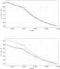Fig. 8 Radial dependence of the modified angular velocity (solid) and the initial angular velocity (broken) at z = 0 at z = 0.05 (broken) at small radii for model l39 with fV = 0.667.

Solutions that converged to a (statistically) steady state could not be found with α defined as in Eq. (18). We thus took α to be non-zero in the disc only, $\begin{array}{ccc}\mathit{\alpha }\mathrm{\left(}\mathit{r,z}\mathrm{\right)}& \mathrm{=}& {\mathit{\alpha }}_{\mathrm{d}}\sin \hspace{0.17em}\mathrm{(}\mathit{\pi z}\mathit{/}{\mathit{h}}_{\mathrm{d}}\mathrm{(}\mathit{r}\mathrm{\left)}\mathrm{\right)}\mathit{,}\mathrm{\left|}\mathit{z}\mathrm{\right|}\mathrm{\le }{\mathit{h}}_{\mathrm{d}}\mathrm{\left(}\mathit{r}\mathrm{\right)}\mathrm{;}\\ \mathit{\alpha }\mathrm{\left(}\mathit{r,z}\mathrm{\right)}& \mathrm{=}& \end{array}$In other words, we have to exclude the exponential tail of the α-distribution in the region surrounding the disc and prescribe zero α-effect in the surrounding space. Such tails were unimportant for the quasi-kinematic problem, however they prevent complete separation of dynamo action in the disc from processes in the surrounding space. As far as we know this point has not been reported in the galactic dynamo studies: arguably it is an outcome of the specific rotation law. (The issue of a separation between disc and halo dynamo actions has been considered in a galactic context by Moss & Sokoloff 2008).

Simultaneously, to obtain convergent solutions, it was found necessary to increase the aspect ratio of the computational box; a ratio of 0.5 was found to be safely adequate to obtain statistically steady states. Now a vertical resolution nk ≥ 16 001 is required, and nk = 16 001 (and ni = 151) was taken for most models. Some solutions were recomputed with nk = 32 001, also with ni increased to 301 and nk = 16 001. Even so taking r_in = 0.01 as in the quasi-kinematical models did not give satisfactory models, and most solutions used r_in = 0.015. (We would have liked to compute solutions with ni = 301, nk = 32 001, but this resolution was inaccessible with the facilities available. Such an increase might allow taking r_in = 0.01.)

In the computations described below, the initial angular velocity associated with the disc model was taken to be independent of z. We did experiment with the possibility of a z-dependent initial angular velocity, but could only find satisfactory solutions when the z-dependence was very weak. Given that the important dynamo action occurs near to the disc, where vertical variations in angular velocity can be expected to be small, we did not pursue this point. Because of these difficulties, computations were now performed in the region z ≥ 0; previous experience strongly suggest that stable solutions are strictly of even parity, at least for not very supercritical states, so we confined our studies to even parity configurations. This is also supported by the work of Rekowski et al. (2000).

Note that the change in definition of α from that in the earlier, quasi-kinematic, models means that the the excitation conditions etc of the two sets of models are not strictly comparable: for example, ^∫αdV over the disc volume is now significantly reduced.

5.2. Results: models with R${\mathit{\alpha }}_{}\mathit{>}\mathrm{0}$

We first investigated models with prescribed even parity. These arise when R_α> 0, i.e. the case where right handed turbulent vortices dominate in the northern hemisphere of the disc. According to modern views of the origin of the α-effect, this case is strongly preferred.

Using the previous notation, with the slightly supercritical value f_v = 0.667 we obtain a strictly steady state, with magnetic field more-or-less smoothly distributed over the disc (model l39). Distortions of the rotation curve are minor, and restricted to the near disc region close to r = r_in. Figure 8 shows the variation with radius of the modified angular velocity and the initial angular velocity on z = 0 and z = 0.05. Figure 9 shows the distribution of the global poloidal and inner toroidal fields. The “wobbles” in the toroidal field distribution in the region above the disc are artefactual, but experiments suggest that they do not appear to depend on the spatial resolution.

Fig. 9 Global solution (left, contours of the poloidal field) and a magnified view of the solution near r = rin (right, contours of toroidal field), for the slightly supercritical parameter for the even parity model with fv = 0.667 – model l39. The dashed curve shows the disc boundary. Here and elsewhere wobbles in contours near the inner disc plane appear artefactual – see the text.

With f_v = 1 (model l28), the global energy develops very small irregular fluctuations (≲0.01%) in the saturated state, and the angular velocity is noticeably modulated by the Lorentz force – see Fig. 10. This effect is again limited to small radii, with a z-extent of a few multiples of the disc height. The energy fluctuations arise from this region. f_v ≈ 1 marks a transition from steady states with field distributed smoothly with radius to fluctuating states with toroidal field concentrated strongly to the inner disc region. The distribution of the ratio of total field strength to equipartition field strength may be more informative: it is shown for the model with f_v = 1 in Fig. 11. Apart from the innermost regions, this distribution does not change greatly as f_v increases.

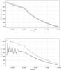Fig. 10 Radial dependence of the modified angular velocity (solid) and the initial angular velocity (broken) at z = 0 at z = 0.05 (broken) at small radii for model l28.

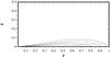Fig. 11 Distribution of the ratio of total field strength to equipartition field strength for model l28. There are departures from the smooth curves only at very small radii. The maximum is approximately 4.2, and contours are at values 1.0, 1.8, 2.6, 3.4.

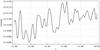Fig. 12 Variation with time of global magnetic energy for model l36 with fV = 1.5.

With f_v = 1.5 (model l36), the global energy has quite irregular fluctuations (Fig. 12), and the field continues to be concentrated in the inner disc region.

Attempts were made to obtain models with larger values of f_v, but then greater spatial resolution than available seems to be required to obtain reliable results. As stated, the “standard” case has resolution 151 × 16 001 grid points. Cases were also run with 301 × 16 001 and 151 × 32 001 points. There were some differences, but these experiments strongly suggest that the trends seen when moving from f_v = 1 to f_v = 1.5 continue for larger values of f_v: the field continues to be concentrated near the inner disc, and this region is the source of the temporal fluctuations.

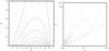Fig. 13 Global solution (left, contours of the poloidal field) and a magnified view of the solution near r = rin (right, contours of toroidal field), for the slightly supercritical odd parity model with fv = 1.0 and negative Rα – model l55. The maximum value of Bφ is approximately 6.4 × 104 G, and the contour spacing is 1.6 × 104 G. The dashed curve shows the disc boundary.

5.3. Results: models with negative R${\mathit{\alpha }}_{}$

We also made a superficial study of models with negative R_α and odd parity, corresponding to domination of left-handed vortices in the northern hemisphere. This appears unrealistic according to contemporary understanding of the origin of the α-effect, but it is difficult to exclude this possibility completely. We took initially f_v = 1, and the poloidal and toroidal fields are shown in Fig. 13 – model l55. The saturated field is steady. The dependence of angular velocity on radius in the inner disc is shown in Fig. 14, and the modulation of angular velocity in the inner disc is small – also (Fig. 14). Fields are not so strongly concentrated to the inner disc. (With prescribed quadrupolar parity and R_α< 0, dynamo excitation occurs at significantly larger dynamo numbers: it is clear that with negative values of R_α even parity solutions are preferably excited.) With f_v = 1.167, there is a transition to temporally unsteady solutions with marked modulation of the angular velocity in the inner disc. Accretion disc dynamo problems with negative R_α were addressed by Rekowski et al. (2000) and here we broadly confirm these results.

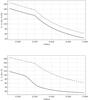Fig. 14 Radial dependence of the modified angular velocity (solid) and the initial angular velocity (broken) at z = 0 at z = 0.05 (broken) at small radii for model l28.

6. Discussion

Simple models of magnetic field excitation in accretion discs and the corresponding dynamo driven magnetic configuration presented above show to some extent a similarity between accretion disc and galactic dynamos; however there are also important differences between them.

At least in the framework of the basic accretion disc model that uses a standard hydrodynamical model for the structure of discs, for smaller dynamo numbers we obtain a dynamo excitation with a steady magnetic field configuration with the axisymmetric magnetic field concentrated near the central plane of the disc and maximal near its inner boundary. The field rapidly decays above and below the disc. The configuration weakly depends on the most prominent parameters responsible for accretion disc hydrodynamics, such as accretion rate, i.e. infall velocities.

At first sight it might look rather unexpected that the steady magnetic field strength is approximately equal to the equipartition field strength. This is a natural consequence of the supercriticality of the dynamo. For example Shukurov (2004) gives the estimate $\begin{array}{ccc}{\mathit{B}}_{\mathrm{steady}}^{\mathrm{2}}\mathrm{~}\mathrm{4}\mathit{\pi \rho }{\mathit{V}}_{\mathit{t}}\mathrm{\Omega }\mathit{l}\mathrm{\left[}\mathrm{\right|}\mathit{D}\mathit{/}{\mathit{D}}_{\mathit{c}}\mathit{r}\mathrm{|}\mathrm{-}\mathrm{1}{\mathrm{]}}^{\mathrm{1}\mathit{/}\mathrm{2}}& & \end{array}$for the saturation field strength. With η = (lV_t) / 3 we get ${\mathit{B}}_{\mathrm{steady}}^{\mathrm{2}}{}^{{\mathrm{\propto }}_{\mathrm{~}}}\mathrm{12}\mathit{\pi \rho \eta }\mathrm{\Omega }$ giving a strong radial dependence r^{− 21 / 8}Q(r)^{17 / 20}.

We can identify the parameter which could be responsible for substantial deviations from the basic model. It is the ratio of the rms turbulent velocity to the sound speed. Because the turbulence is hardly supersonic, the ratio σ_v is expected to be lower then unity. If the ratio σ_v ≈ 0.3 (rms turbulent velocity is 3 times lower then the sound speed) the magnetic configuration becomes unsteady, and has irregular oscillations with time scale of about 0.2 diffusion times. However magnetic field is still concentrated at the equatorial plane. Such behaviour is unknown for galactic dynamos, maybe because of the lack of interest in and immediate physical relevance of such behaviour. An additional point is that we only have snapshots of actual galactic magnetic fields.

If we accept that the rms turbulent velocity is about one order of magnitude lower than the sound speed then, at least in the absence of feedback on the rotation curve from the Lorentz force, the magnetic configuration departs from strict quadrupolar symmetry and the magnetic field maxima are found near the upper and lower boundaries of the disc, rather at the central disc plane. There are again irregular oscillations with dimensionless time scale slightly smaller than in the previous case. Such magnetic configurations are unknown for galactic dynamos. The key point here appears to be that galactic turbulence is believed to have rms velocity close to the sound speed.

Taking into account the possibility that the nature of the mirror asymmetry of accretion disc turbulence is more complicated then just a straightforward action of Coriolis force in a stratified medium, we here considered what happens if this mirror asymmetry has sign opposite to the conventional expectation. We show in Fig. 7 the field when f_V = 0.25. Then the dynamo driven magnetic field is steady with dipolar symmetry and the magnetic field maxima (in practice, maxima of the toroidal field which has to vanish at the disc plane) are located above and below the disc.

We have also made a preliminary study of the effects of the Lorentz force arising from the large-scale magnetic field on the rotational velocities. Except in the innermost disc, these effects are small. Generally, the overall conclusions are little altered. The irregular behaviour begins to occur at slightly larger formal values of the dynamo numbers, but given the inherent uncertainty in the modelling, including the change in definition of α(r,z), this is hardly physically significant.

We remphasize here that the models with f_v< 1 correspond formally at least to the physically unrealistic case of supersonic turbulence in the disc. These include most of the steady solutions. On the other hand, solutions with f_v> 1, corresponding formally to subsonic turbulence, are more-or-less invariably irregular, both without and with the inclusion of the Lorentz force feedback on the rotation. However, although we are unable to follow the latter class of solutions satisfactorily there are strong indications that significant modifications of the rotation law will be present. In turn this means that to follow the evolution of these solutions self consistently, real time updating of the disc model would be required.

We note that numerical implementation even for our the simple models is relatively demanding of computer facilities. Making a crude estimate of what would be required for a direct numerical simulation of the type of magnetic configurations discussed, assuming as a quite modest requirement that simulation of a box of the size H × H × H would require 100³ mesh point and that the disc aspect ratio is 10^-2, we conclude that simulation of magnetic field equation in the whole disc would require about 2 × 10¹¹ equations, as well as equations for hydrodynamic quantities, description of the disc environment, etc. A quite moderate estimate suggests that such straightforward approach would be a very complicated undertaking and investigation of simple mean-field models such as described above as an adjunct to direct numerical simulation looks reasonable. Of course, the simple models have specific limitations as well. In particular, it is difficult to believe that we take into account even the more important, not to say all, instabilities which result in irregular oscillation.

In the framework of this paper we assume that the accretion disc is thin. This does not include all options discussed in accretion disc studies and we recognize the possibility that magnetic field generation occurs in the central part of a thick disc. A natural expectation from dynamo studies is that then the magnetic field configuration will be an oscillating dipole with magnetic field concentrated far above and below the disc central plane; however verification of this expectation would require separate modelling which considers quasispherical configurations of dynamo drivers. This is obviously beyond the scope of this paper.

Of course, a detailed comparison of the above results with available observations of cataclysmic variables deserves a special investigation. At least, however, magnetic configurations obtained in the basic model appear coherent in the framework of the standard Shakura & Sunyaev (1973) theory.

6.1. Possible astrophysical applications

We now discuss in more detail the oscillations in total magnetic energy present in more supercritical dynamo regimes. Much of this discussion is based on the models without Lorentz force, discussed in Sect. 4: the numerical limitations mentioned make it difficult to compute these models for very supercritical values. However indications are that the basic nature of the results will not change significantly, within the intrinsic limitations and uncertainties of the modelling.

The corresponding characteristic time scale of the oscillations is about 0.2–0.4 of the diffusion time scale. As the total (thermal plus magnetic) energy in the disc is conserved, the thermal energy in the disc must oscillate with the same characteristic time. Thus the oscillations of the magnetic energy could lead to quasi-periodic oscillations (QPOs) of the accretion disc luminosity.

Our computations demonstrate that the magnetic energy is concentrated near the inner radii of accretion discs. The maximum radiation flux also emerges at this accretion disc region. Therefore, we can expect that QPO character times could be close to 20–40% of the diffusion time scale characteristic of the inner parts of the disc.

For the inner parts of the accretion discs around white dwarfs the corresponding characteristic time is a few tens of seconds (see Eq. (15)). The coherent oscillations of high-degree with similar periods observed during dwarf nova outbursts are well known. They have periods 7–40 s and are known as dwarf nova oscillations (DNOs; see Warner 2003). Our accretion discs have the high accretion rate typical of dwarf novae during outbursts. Therefore, we can suggest that the magnetic energy oscillations found are connected with DNOs and could explain them.

Most of the existing models suggested to explain DNOs are connected with various instabilities in the optically thick boundary layer between the accretion disc and the white dwarf (Godon 1995; Collins et al. 1998; Popham 1999; Piro & Bildsten 2004). It is interesting, that the model suggested by Warner & Woudt (2002) describes DNOs using a magnetic field in the boundary layer (a low-inertia magnetic accretor model).

Optically thick accretion discs also exist around much more compact objects: neutron stars and black hole candidates (low-mass X-ray binaries, LMXBs). Quasi-periodic oscillations of X-ray flux are observed in LMXBs with neutron stars and they are known as kHz QPOs (in the range 200–1200 Hz, and usually occuring in pairs, see the review by van der Klis 2000). We note that the diffusion time-scale at the LMXB inner disc radii, which is close to the Kepler time scale, is much smaller than in cataclysmic variables, and is comparable with the observed kHz QPO periods 10^-2–10^-3 s. Therefore, the observed kHz QPOs can be also associated with the total magnetic energy oscillations in the accretion discs.

We do not propose any new model for DNOs (or kHz QPOs). We have just found magnetic energy oscillations in accretion discs due to dynamo action, with typical time scales close to the periods of DNOs or kHz QPOs.

There are some sources of uncertainties, which prevent us from claiming a definitive new DNO model. First is the nature of the z-dependence of the angular velocity. The limited experimentation mentioned above suggests that this may not be too important, but more cannot be stated. Another rather arbitrary feature of the model is the nature of the inner boundary conditions but, again, limited experimentation suggests that solutions are not very sensitive to “reasonable” choices.

An extension of our results to the accretion discs of black holes seems a natural further step for investigation. Treatment of the whole disc in a 2D model may be a quite challenging numerical problem, given the larger radial range and greater range of variation in disc thickness. Given our experiences here, further progress might be made by just modelling the innermost disc in a thin computational domain.

7. Conclusions

A limitation of our models is the plausible restriction to axisymmetry. Nevertheless, by including a realistically thin disc that extends inwards to near the boundary of the central accreting object we have demonstrated the importance of including the whole disc in the model: radially truncated discs omit the region of maximum magnetic field and the irregular fluctuations arise from this region, especially in the models with Lorentz force. We have been able to explore a range of possibilities for the dynamo number, and have found quadrupolar type solutions with irregular temporal oscillations that might be compared to observed rapid fluctuations (DNOs). These oscillations exist both in the models with only the alpha-quenching non-linearity and also for those with the addition of the Lorentz force feedback. The dipolar symmetry models with R_α< 0 (Sect. 4.6) have lobes of strong toroidal field adjacent to the rotation axis that could be relevant to jet launching phenomena. In short, we have explored and extended the solutions known for thin accretion discs around compact objects.

Acknowledgments

V.S. thanks DFG for financial support (grant WE 1312/48-1) and D.S. thanks RFBR for support (grant 15-02-01407) and Eberhard Karls Universität, Tübingen for its hospitality. Criticisms from the referee led to significant improvement of the paper.

References

Appendix A: Appendix A

We recall here some definitions associated with decomposition of dynamo generated magnetic configurations into symmetry types with respect to the disc plane. Let z = 0 be the central plane of an accretion disc in a Cartesian reference frame x,y,z. Define the even and odd parts of a scalar S(x,y,z) by S_even = (S(x,y,z) + S(x,y, − z)) / 2 and S_odd = (S(x,y,z) − S(x,y, − z)) / 2. If B(x,y,z) is a magnetic field, then define ${\mathit{E}}_{\mathrm{even}}\mathrm{=}{}^{\mathrm{\int }}\mathrm{(}{\mathit{B}}_{\mathit{x,}\mathrm{even}}^{\mathrm{2}}\mathrm{+}{\mathit{B}}_{\mathit{y,}\mathrm{even}}^{\mathrm{2}}\mathrm{+}{\mathit{B}}_{\mathit{z,}\mathrm{odd}}^{\mathrm{2}}\mathrm{)}\mathit{/}\mathrm{\left(}\mathrm{8}\mathit{\pi }\mathrm{\right)}\mathrm{d}\mathit{V}$ and correspondingly ${\mathit{E}}_{\mathrm{odd}}\mathrm{=}{}^{\mathrm{\int }}\mathrm{(}{\mathit{B}}_{\mathit{x,}\mathrm{odd}}^{\mathrm{2}}\mathrm{+}{\mathit{B}}_{\mathit{y,}\mathrm{odd}}^{\mathrm{2}}\mathrm{+}{\mathit{B}}_{\mathit{z,}\mathrm{even}}^{\mathrm{2}}\mathrm{)}\mathit{/}\mathrm{\left(}\mathrm{8}\mathit{\pi }\mathrm{\right)}\mathrm{d}\mathit{V}$. The mixing of odd and even parts in these expressions is a consequence of an alpha-effect dynamo with α-coefficient that is odd with respect to the plane z = 0. The integrals are in principle taken over the whole space and in practice over the computational domain.

All Figures

	Fig. 1 Global solution (left) and a magnified view of the solution near r = rin (right), for the slightly supercritical parameters Rα = 0.6, Rω = 15, Rm = 0.146. In upper panels solid line is for Beq and dashed line stands for Bφ.
In the text

Fig. 2 Global solution (left, contours of the poloidal field) and a magnified view of the solution near r = rin (right, contours of toroidal field), for the somewhat supercritical parameters in the 2D model (fv = 0.3). Even parity, P = + 1. In this and subsequent figures, contours are equally spaced, solid contours correspond to positive values, broken contours represent negative values, and the dashed curve shows the disc boundary. In the right hand panel the maximum toroidal field strength occurs at r ≈ 0.015,z = 0 and is approximately 4 × 105 G. The contour interval is approximately 8 × 104 G. In all the models the poloidal field is weaker: here the mean global ratio of poloidal to toroidal field strengths is about 10-2. In this and subsequent figures, the field strength beyond the outermost contour is smaller than that at the outermost contour.

In the text

	Fig. 3 Temporal behaviour of the total global magnetic energy for Rα = 0.6, fv = 1. Even parity, P = + 1. (Energy is normalized with the equipartition energy at the outer radius – see Eq. (9).) Energy here and below is calculated by integration over the whole entire computaional volume (see Appendix for details).
In the text

Fig. 4 Solution with Rα> 0,fv = 1, even parity P = + 1. The contours lines of Bφ near the inner boundary (top panel), the poloidal field lines in the complete computational space (middle) and contours of the ratio | Bφ | /Beq (bottom). In the top panel the maximum of the toroidal field strength is about 2.4 × 105 G, and the contour spacing is approximately 4 × 104 G. In the lower panel the maximum of | B | /Beq is about 0.6 at r ≈ 0.15,z = 0, with contour spacing 0.12. In this and subsequent figures, contours are equally spaced.

In the text

	Fig. 5 Temporal behaviour of the total global magnetic energy for fv = 2; solution with free parity. The upper panel shows the evolution of the parity P, the middle panel the ratio of poloidal to toroidal energies, and the lower panel the evolution of the total magnetic energy.
In the text

	Fig. 6 2D solution with free parity and Rα> 0,fv = 2; the computation extends over −zm ≤ z ≤ zm. The contour lines of Bφ near the inner boundary (left) and poloidal field lines (right) in the complete computational space.
In the text

	Fig. 7 Solution with Rα< 0,fv = 0.25, odd parity P = −1. The contour lines of Bφ near the inner boundary (left) and the poloidal field lines in the complete computational space (right). The maximum value of | Bφ | is approximately 7.2 × 105 G, and the contour spacing is 1.2 × 105 G. The mean global ratio of poloidal to toroidal field strength is about 3 × 10-3.
In the text

	Fig. 8 Radial dependence of the modified angular velocity (solid) and the initial angular velocity (broken) at z = 0 at z = 0.05 (broken) at small radii for model l39 with fV = 0.667.
In the text

	Fig. 9 Global solution (left, contours of the poloidal field) and a magnified view of the solution near r = rin (right, contours of toroidal field), for the slightly supercritical parameter for the even parity model with fv = 0.667 – model l39. The dashed curve shows the disc boundary. Here and elsewhere wobbles in contours near the inner disc plane appear artefactual – see the text.
In the text

	Fig. 10 Radial dependence of the modified angular velocity (solid) and the initial angular velocity (broken) at z = 0 at z = 0.05 (broken) at small radii for model l28.
In the text

	Fig. 11 Distribution of the ratio of total field strength to equipartition field strength for model l28. There are departures from the smooth curves only at very small radii. The maximum is approximately 4.2, and contours are at values 1.0, 1.8, 2.6, 3.4.
In the text

	Fig. 12 Variation with time of global magnetic energy for model l36 with fV = 1.5.
In the text

	Fig. 13 Global solution (left, contours of the poloidal field) and a magnified view of the solution near r = rin (right, contours of toroidal field), for the slightly supercritical odd parity model with fv = 1.0 and negative Rα – model l55. The maximum value of Bφ is approximately 6.4 × 104 G, and the contour spacing is 1.6 × 104 G. The dashed curve shows the disc boundary.
In the text

	Fig. 14 Radial dependence of the modified angular velocity (solid) and the initial angular velocity (broken) at z = 0 at z = 0.05 (broken) at small radii for model l28.
In the text

References

- Arlt, R., & Rüdiger, G. 2001, A&A, 374, 1035 [NASA ADS] [CrossRef] [EDP Sciences] [Google Scholar]
- Balbus, S. A., & Hawley, J. F. 1991, ApJ, 376, 214 [NASA ADS] [CrossRef] [Google Scholar]
- Blackman, E. 2012, Phys. Scr., 86, 058202 [NASA ADS] [CrossRef] [Google Scholar]
- Blandford, R. D., & Payne, D. G. 1982, MNRAS, 199, 883 [NASA ADS] [CrossRef] [Google Scholar]
- Blandford, R. D., & Znajek, R. L. 1977, MNRAS, 179, 433 [NASA ADS] [CrossRef] [Google Scholar]
- Brandenburg, A., Nordlund, A., Stein, R., & Torkelsson, U. 1995, ApJ, 446, 741 [NASA ADS] [CrossRef] [Google Scholar]
- Chamandy, L., Shukurov, A., Subramanian, K., & Stoker, K. 2014, MNRAS, 443, 1867 [NASA ADS] [CrossRef] [Google Scholar]
- Collins, T. J. B., Helfer, H. L., & Van Horn, H. M. 1998, ApJ, 508, L159 [NASA ADS] [CrossRef] [Google Scholar]
- Davis, S. W., Stone, J. M., & Pessah, M. E. 2010, ApJ, 713, 52 [NASA ADS] [CrossRef] [Google Scholar]
- Godon, P. 1995, MNRAS, 274, 61 [NASA ADS] [CrossRef] [Google Scholar]
- Gressel, O., & Pessah, E. 2015, ApJ, 810, 59 [NASA ADS] [CrossRef] [Google Scholar]
- Hertfelder, M., Kley, W., Suleimanov, V., & Werner, K. 2013, A&A, 560, A56 [NASA ADS] [CrossRef] [EDP Sciences] [Google Scholar]
- Jiang, Y.-F., Stone, J. M., & Davis, S. W. 2013, ApJ, 767, 148 [NASA ADS] [CrossRef] [Google Scholar]
- Kleeorin, N., Moss, D., Rogachevskii, I., & Sokoloff, D. 2000, A&A, 361, L5 [NASA ADS] [Google Scholar]
- Kleeorin, N., Moss, D., Rogachevskii, I., & Sokoloff, D. 2002, A&A, 387, 453 [NASA ADS] [CrossRef] [EDP Sciences] [Google Scholar]
- Kleeorin, N., Moss, D., Rogachevskii, I., & Sokoloff, D. 2003, A&A, 400, 9 [NASA ADS] [CrossRef] [EDP Sciences] [Google Scholar]
- Lubow, S. H., Papaloizou, J. C. B., & Pringle, J. E. 1994, MNRAS, 267, 235 [NASA ADS] [Google Scholar]
- Moss, D. 1995, MNRAS, 275, 191 [NASA ADS] [Google Scholar]
- Moss, D., & Brooke, J. 2000, MNRAS, 315, 521 [NASA ADS] [CrossRef] [Google Scholar]
- Moss, D., & Shukurov, A. 2004, A&A, 413, 403 [NASA ADS] [CrossRef] [EDP Sciences] [Google Scholar]
- Moss, D., & Sokoloff, D. 2008, A&A, 413, 403 [Google Scholar]
- Moss, D., & Tuominen, I. 1990, A&A, 487, 197 [Google Scholar]
- Narayan, R., McClintock, J. E., & Tchekhovskoy, A. 2014, in General Relativity, Cosmology and Astrophysics, eds. J. Bičák, & T. Ledvinka, 523 [Google Scholar]
- Nauenberg, M. 1972, ApJ, 175, 417 [NASA ADS] [CrossRef] [Google Scholar]
- Okuzumi, S., Takeuchi, T., & Muto, T. 2014, ApJ, 785, 127 [NASA ADS] [CrossRef] [Google Scholar]
- Pariev, V. I., & Colgate, S. A. 2007, ApJ, 658, 129 [NASA ADS] [CrossRef] [Google Scholar]
- Phillips, A. C. 2000, J. Roy. Astron. Soc. Canada, 94, 135 [Google Scholar]
- Piro, A. L., & Bildsten, L. 2004, ApJ, 610, 977 [NASA ADS] [CrossRef] [Google Scholar]
- Popham, R. 1999, MNRAS, 308, 979 [NASA ADS] [CrossRef] [Google Scholar]
- Popham, R., & Narayan, R. 1995, ApJ, 442, 337 [NASA ADS] [CrossRef] [Google Scholar]
- Pringle, J. E., & Savonije, G. J. 1979, MNRAS, 187, 777 [NASA ADS] [CrossRef] [Google Scholar]
- Rekowski, M. V., Rüdiger, G., & Elstner, D. 2000, A&A, 353, 813 [NASA ADS] [Google Scholar]
- Reyes-Ruiz, M., & Stepinski, T. F. 1999, A&A, 342, 892 [NASA ADS] [Google Scholar]
- Rüdiger, G., Elstner, D., & Stepinski, T. F. 1995, A&A, 298, 934 [NASA ADS] [Google Scholar]
- Sadowski, A., Narayan, R., Tchekhovskoy, A., et al. 2015, MNRAS, 447, 49 [NASA ADS] [CrossRef] [Google Scholar]
- Shakura, N. I., & Sunyaev, R. A. 1973, A&A, 24, 337 [NASA ADS] [Google Scholar]
- Shukurov, A. 2004, ArXiv e-prints [arXiv:astro-ph/0411739] [Google Scholar]
- Sokoloff, D., & Shukurov, A. 1990, Nature, 347, 51 [NASA ADS] [CrossRef] [Google Scholar]
- Stepinski, T. F., & Levy, E. H. 1990, ApJ, 362, 318 [NASA ADS] [CrossRef] [Google Scholar]
- Stone, J. M., Hawley, J. F., Gammie, C. F., & Balbus, S. A. 1996, ApJ, 463, 656 [NASA ADS] [CrossRef] [Google Scholar]
- Subramanian, K., & Mestel, L. 1993, MNRAS, 265, 649 [NASA ADS] [CrossRef] [Google Scholar]
- Suleimanov, V. F., Lipunova, G. V., & Shakura, N. I. 2007, Astron. Rep., 51, 549 [NASA ADS] [CrossRef] [Google Scholar]
- Torkellson, U., & Brandenburg, A. 1994, A&A, 283, 677 [NASA ADS] [Google Scholar]
- Tylenda, R. 1977, Acta Astron., 27, 235 [NASA ADS] [Google Scholar]
- van der Klis, M. 2000, ARA&A, 38, 717 [NASA ADS] [CrossRef] [Google Scholar]
- Warner, B. 2003, Cataclysmic Variable Stars (Cambridge, UK: Cambridge University Press) [Google Scholar]
- Warner, B., & Woudt, P. A. 2002, MNRAS, 335, 84 [NASA ADS] [CrossRef] [Google Scholar]