| Issue |
A&A
Volume 587, March 2016
|
|
|---|---|---|
| Article Number | A112 | |
| Number of page(s) | 17 | |
| Section | Catalogs and data | |
| DOI | https://doi.org/10.1051/0004-6361/201526676 | |
| Published online | 26 February 2016 | |
Long-term R and V-band monitoring of some suitable targets for the link between ICRF and the future Gaia celestial reference frame⋆
1 Observatoire de Paris – SYRTE, PSL Research University, CNRS/UMR 8630, Sorbonne Universités, Université Pierre et Marie Curie, LNE, 61 avenue de l’Observatoire, 75014 Paris, France
e-mail: Francois.Taris@obspm.fr
2 Observatório Nacional/MCT, 11 Rio de Janeiro, Brasil
3 Obervatorio do Valongo, UFRJ, 43 – Centro, Rio de Janeiro, Brasil
4 Institut d’Astrophysique, UPMC Univ. Paris 6, CNRS, UMR 7095, 98bis Bd Arago, 75014 Paris, France
5 Université de Toulouse, UPS/OMP, IRAP, 31400 Toulouse, France
6 CNRS, IRAP, 14 avenue Édouard Belin, 31400 Toulouse, France
7 Observatoire de Paris – IMCCE, 75252 Paris, France
Received: 4 June 2015
Accepted: 3 December 2015
Context. The Gaia astrometric mission of the European Space Agency was launched on December 2013. It will provide a catalog of 500 000 quasars. Some of these targets will be chosen to build an optical reference system that will be linked to the International Celestial Reference Frame (ICRF). The astrometric coordinates of these sources will have roughly the same uncertainty at both optical and radio wavelengths, and it is then mandatory to observe a common set of targets to build the link. In the ICRF, some targets have been chosen because of their pointlikeness. They are quoted as defining sources, and they ensure very good uncertainty about their astrometric coordinates. At optical wavelengths, a comparable uncertainty could be achieved for targets that do not exhibit strong astrophysical phenomena, which is a potential source of photocenter flickering. A signature of these phenomena is a magnitude variation at optical wavelengths.
Aims. The goal of this work is to present the time series of 14 targets suitable for the link between the ICRF and the future Gaia Celestial Reference Frame. The observations have been done systematically by robotic telescopes in France and Chile once every two nights since 2011 and in two filters. These time series are analyzed to search for periodic or quasi-periodic phenomena that must be taken into account when computing the uncertainty about the astrometric coordinates.
Methods. Two independent methods were used in this work to analyze the time series. We used the CLEAN algorithm to compare the frequency obtained to those given by the Lomb-Scargle method. It avoids misinterpreting the frequency peaks given in the periodograms.
Results. For the 14 targets we determine some periods with a confidence level above 90% in each case. Some of the periods found in this work were not previously known. For the others, we did a comparative study of the periods previously studied by others and always confirm their values. All the periods given by the two methods are in good agreement with the difference always below 7.9% in the worst case. Finally we also present the structure functions for our two sets of objects (BL Lac and Seyfert galaxies).
Conclusions. For all but one target, we find variations that could be the signature of periodic or quasi-periodic phenomena. Our time series could allow to bring some constraints on astrophysical models that could explain such variations. Binary black hole system, instabilities in the jet or in the accretion disk, changes in the torus structure are some of these astrophysical phenomena. They must be kept in mind when evaluating the uncertainty about the astrometric position of the targets suitable for the link between reference systems in a conservative way.
Key words: reference systems / astrometry / quasars: general
Full Tables 5 and 6 are only available at the CDS via anonymous ftp to cdsarc.u-strasbg.fr (130.79.128.5) or via http://cdsarc.u-strasbg.fr/viz-bin/qcat?J/A+A/587/A112
© ESO, 2016
1. Introduction
The European astrometric space mission Gaia was launched on December 19, 2013. It will provide positions of around 500 000 quasars with an unprecedented uncertainty between the 6th and the 20th magnitudes (de Bruijne 2012). According to Perryman et al. (2014), the expected accuracy of the frame spin (residual rotation) would be 0.5 μas/yr. It would be at the level of 10 μas for the frame orientation. It must be noted that these two values also depend on the source instability, which is currently not very well known.
On the other hand, the current International Celestial Reference Frame (ICRF) is based on the observations of extragalactic sources at radio wavelengths.
At the 2009 XXVIIth IAU General Assembly in Rio, Brazil, the astronomical community adopted the second release of the International Celestial Reference Frame named ICRF2 (Fey et al. 2009) as the new fundamental astrometric materialization of the ICRS. From January 1, 2010, the ICRF2 replaces the ICRF (Ma et al. 1998) and its more recent extension, the ICRF-Ext2 (Fey et al. 2004).
The construction of the ICRF2 used almost 30 yr of geodetic very long baseline interferometry (VLBI) observations at 3.6 cm and 13 cm wavelengths. The ICRF2 catalog contains the positions of 3414 compact radio sources. The formal errors σ in source coordinates were inflated according to  where σ0 is a noise floor set to 40 μas. The median error in the position of sources observed in more than two sessions is 175 μas. The frame axes are defined by the coordinates of 295 “defining” sources with a stability of ~10 μas. The defining sources were chosen on the basis of their high positional stability and low structure index. A subset of 138 defining sources was used to align the ICRF2 catalog onto the previous ICRF.
The ICRF2 currently represents the most accurate realization of the celestial system with respect to which the position of any object in the celestial sphere should be measured. We note that the ICRF2 is epochless and independent of the dynamical frame (ecliptic) and reference point (equinox), but is consistent with previous realizations of the ICRS, including the FK5 J2000.0 optical system.
The astrometric coordinates of sources in both radio and optical reference frames will have roughly the same uncertainty. It is then mandatory to observe a set of common targets at both optical and radio wavelengths to link the ICRF with what could be called the Gaia Celestial Reference Frame (GCRF). The work on the link between radio and optical reference system is achieved in the framework of the ICRS Product Center of the IERS. It has been shown that a clean sample of less than 10 000 quasars could stabilize the axes of the future GCRF at a level of 0.5 μas/yr, with the assumption that the random instability of the sources is less than 20 μas (Mignard 2002). This random instability is a very stringent limit and the chosen targets must be carefully scrutinized both from the points of view of morphology and photometry.
The unified model for the active galactic nuclei (AGN) is a well known and adopted model for a set of different observational classes of objects. It postulates that the appearance of AGN depends strongly of the orientation of the line of sight in addition to intrinsic physical properties. It is described, for example, by Antonucci (1993) and Urry & Padovani (1995). The AGN class includes a priori different objects, such as blazars, radio loud or radio quiet quasars, Seyfert galaxies, and narrow or broad line radio galaxies. They are all linked by some common physical components, such as a black hole (eventually a binary one), an accretion disk, broad and narrow line regions, an obscuring torus, and a jet.
For a very long time, AGN have been presented as unchanging point-like objects at optical wavelengths because they were extragalactic sources at cosmological distances. With that point of view they can materialize a quasi inertial celestial reference frame.
Nevertheless it has been pointed out that at radio wavelengths these objects are not point-like sources and that a structure index (Fey & Charlot 2000) can be computed. The intrinsic and extended radio structure of the extragalactic radio sources, and its evolution, is one of the limiting factors for the definition of the ICRF reference frame. Sources are classified as defining sources (which served to set the axes of the frame), candidate sources (less observed), or other sources. A significant proper motion has been pointed out by Fey et al. (1997) in the case of the source 4C 39.25. This motion is due to intrinsic source structure changes. As a matter of fact, the position instabilities of the radio center makes some sources inadequate for fulfilling the conditions of defining sources during some given period of time. For this reason the monitoring of the ICRF sources is a task currently in progress in the framework of the International Earth Rotation Service-Product Center (IERS-PC1) and the International VLBI Service-Observatoire de PARis (IVS-OPAR2).
As in the radio wavelengths, a morphological index has been defined in the optical wavelengths (Souchay et al. 2012). It gives some indications about the pointlikeness of an object.
The next two sections of this paper are devoted to astrophysical phenomena that could be at the origin of the optical flux variation and to problems linking the radio and optical reference frames.Then, in the fourth section, the telescopes and the data are presented together with the statistical methods used to analyze the flux variation. Finally the structure functions of our two sets of objects (BL Lac and Seyfert galaxies) will be computed just before a conclusion and some prospects about this work.
2. Astrophysical phenomena involved in the optical flux variation of quasars
The optical emission of extragalactic objects, namely galaxies, radio galaxies, QSOs (quasi-stellar objects) and quasars3 (quasi-stellar radio sources) is due to the stellar emission, the emission lines clouds (narrow line region and broad line region), the black body emission of the central part of the accretion disk, the re-emission from the dust torus or sparse dust clouds around the accretion disk, and the optical emission of non-thermal processes (synchrotron and inverse Compton emissions).
Since we are interested on the compact optical objects that will allow us to link the Gaia reference frame with the ICRF reference frame, we limit ourselves to the quasars. We therefore exclude galaxies, radio-galaxies, and QSOs.
The spectrum of quasars is characterized by a power law distribution that extends from the radio range to the γ rays, while the optical emission of quasars shows linear polarization. These characteristics indicate that their optical emission is dominated by non-thermal processes.
Quasars are characterized by ejections of VLBI components. We describe the ejection of a VLBI component in the framework of the two-fluid model (Sol et al. 1989; Pelletier & Roland 1989; 1990; Pelletier & Sol 1992), so we assume that:
-
1.
The outflow consists of an e− − e+ plasma (hereafter the beam) moving at a highly relativistic speed (with corresponding Lorentz factor4γb ≤ 30) surrounded by an e−–p plasma (hereafter the jet) moving at a mildly relativistic speed of vj ≤ 0.4 × c.
-
2.
The magnetic field lines are parallel to the flow in the beam and the mixing layer, and the magnetic field in the jet becomes rapidly toroidal as a function of distance from the core.
The relativistic e± is responsible for the formation of superluminal sources and their optical, X-ray and γ-ray emissions. The e−–p jet carries most of the mass and the kinetic energy ejected by the nucleus. It is responsible for forming kpc-jets, hot spots, and extended lobes.
Because the emitting plasma is ejected relativistically, the emission is anisotropic (Doppler boosted).We suppose that there is a quasi-continuous ejection of relativistic e− − e+ in the beam. The ejection of a VLBI component corresponds to an increase in the density of the ejected relativistic e− − e+. The radio and the optical variability of quasars is produced by a variation in the ejection direction of the relativistic e− − e+ beam and/or a variation in the ejection of the density and/or the energy of the e− − e+ in the beam, particularly when a new VLBI component is ejected.
The VLBI core is the region of the jet that becomes transparent to the synchrotron radiation. The distance between the central black hole (BH) and the VLBI core is unknown and variable. This distance reduces when the frequency of the observations increases. The position of the VLBI core changes with time when the characteristics of the beam changes. Similarly, the optical core is the region of the jet that becomes transparent. It is closer of the central black hole than the VLBI core. Again, the distance between the central BH and the optical core is unknown.
The uncertainties due to differences of the positions of the central BH, the optical core, and the VLBI core depend of the inclination angle. They are smaller when the inclination angle is small, meaning that the quasar is face on.
They are four different kinds of variability observed in optical. They are:
Intraday variability:
Intraday variability (IDV) describes flux-density variations in the radio regime on timescales of a day and less. When they are observed in the radio regime alone, they are explained by refractive interstellar scattering. However, in the case of S5 0716+714, correlated variations at frequencies in the radio and the optical regimes indicate an intrinsic component to the variability. Roland et al. (2009) found that the formation and the rotation of a warp in the inner part of the accretion disk produce a small perturbation of the relativistic beam and consequently a variation in the viewing angle and in the beamed synchrotron emission explaining IDV variations.
Observation of narrow emission peaks of one to two magnitudes separated by several months to one year:
Occasionally, when a new VLBI component is ejected, one observes in the optical, the formation of narrow emission peaks of one to two magnitudes separated by several months to one year. Their relation to the ejection of a new VLBI component has been studied and explained in the case of radio sources PKS 0420-014 (Britzen et al. 2001) and 3C 345 (Lobanov & Roland 2005). It has been shown that this optical emission can be modeled as the synchrotron or inverse Compton emission of a point source ejected in the perturbed beam. This short burst of very energetic relativistic e± happens at the beginning of the ejection of a new VLBI component and is followed immediately by a very long burst of less energetic relativistic e±. This long burst is modeled as an extended structure along the beam and is responsible for the radio emission of the VLBI component.
Observation of long term variability with a quasi-period of several years:
Optical or radio light curves of quasars can often show variability over several years with a quasi-periodic behavior. Sometimes this quasi-period is interpreted as the orbital period of a BBH system in the nucleus of the quasar. Orbital periods of few years imply orbits so close that that the two BH orbit inside the accretion disk. However, modeling the ejection of VLBI components show that the nuclei of extragalactic radio sources contain binary black hole systems whose orbital period is typically between several hundred years to several thousand years and the distance that two BH are separated is larger than the size of the accretion disk.
Quasars can show a radio light curve similar to their optical light curve; that is, one can observe a quasi-period behavior. A careful analysis of the ejection of the VLBI components shows that this quasi period is probably related to the ejection of new VLBI components.
Absorption features observed on a typical time scale of one day:
Optical light curves of quasars sometimes show narrow absorption features during one or two days: for instance, 1424+240 and 0405-123. These absorption lines are produced by small clouds of matter passing in front of the optical core.
3. Problems to link the Gaia reference frame with the ICRF reference frame
Every time that there were VLBI data that were good enough to model the ejection of VLBI components, we found that the nucleus of the radio source contain a BBH system (Britzen et al. 2001 for 0420-014; Lobanov & Roland 2005 for 3C 345; Roland et al. 2008 for 1803+784, Roland et al. 2013 for 1823+568 and 3C 279, and Roland et al. 2015 for 1928+738).
Because radio sources are associated with elliptical galaxies and quasars are a small fraction of QSO (non-radio quasars), one can expect that all quasars contain a BBH system. After the merging of two galaxies, if a BBH system forms, it evolves rapidly to reach a critical radius Rbin ~ 1 pc. After it loses energy emitting gravitational waves, it takes several billion years to collapse (Britzen et al. 2001). This explains why the typical size of the BBH system found in nuclei of extragalactic radio sources is 0.25 pc ≤ Rbin ≤ 1.5 pc (Roland 2014). A typical BBH system with size ≈ 1 pc that contains two similar black holes of 108M⊙ is characterized by an orbital period of 6600 yr.
The position of radio sources as measured by geodetic VLBI shows displacements larger than 0.1 mas in rms (Fig. 1). This lower limit is obviously not only due to changes in the radio source structure: several other limiting factors like the mismodeling of the troposphere wet delay and the noise introduced by site-dependent correlated errors play non-negligible roles.
Using a limited sample, Roland (2014) found that the size of the BBH systems is generally larger than 0.1 mas and that the corresponding rms of the coordinate time series is greater than the size of the BBH systems. If the two black holes are ejecting VLBI components, one can expect significant displacements of the radio center detected by geodetic VLBI, displacements close to the size of the BBH system. If so, it is likely that the astrometric precision of VLBI will be limited in the future by the size of the BBH systems, even at frequencies higher than the current 8.6 GHz band used for the ICRF2. The determination of the number and sizes of BBH systems in quasar nuclei will therefore be crucial in the future realization of reference frames, especially for the choice of the so-called “defining sources” that define the system axes and that should be, in principle, as point-like as possible.
It is fundamental to note that the optical bright quasars have very large Δrms (for instance, the Δrms of the coordinates are, for 3C 273, Δrmsα≈ 1 mas and Δrmsδ≈ 2.9 mas; for 3C 279, Δrmsα≈ 0.75 mas and Δrmsδ≈ 1.5 mas; and for 3C 345, Δrmsα≈ 0.68 mas and Δrmsδ≈ 1.4 mas, Lambert, priv. comm.); that is, the nearby quasars are very poor astrometric sources. The most stable and compact quasars are distant quasars, that is to say, the faint quasars with large magnitudes.
If the nucleus of the radio quasar contains a BBH system and if the two black holes are active, three different situations can occur:
-
1.
The radio core and the optical core are associated with the sameBH. The distances between the radio core and the BH and thedistance between the optical core and the BH are unknown. Thedistance between the radio core and the optical core depends onthe opacity effect, which will be small if the inclination angle issmall.
-
2.
The radio core and the optical core are associated with different black holes. Then the distance between the radio core and the optical core is more or less the size of the BBH system (corrected by the possible opacity effect).
-
3.
The two black holes are emitting at optical wavelength, and then Gaia will provide a mean position between the two optical cores. This position will be different from the positions of the two radio cores.
Since quasars are strongly and rapidly variable, during the five years of observations of Gaia, the three different cases can occur for any given source.
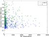 |
Fig. 1 Rms of the coordinate time series of the most observed quasars in the geodetic VLBI monitoring program of the International VLBI Service for Geodesy and Astrometry (IVS; Lambert, priv. comm.) as a function of the number of sessions. |
4. Data and telescopes used in the framework of this study
The two next sections briefly describe the telescopes used to obtain the observational data.
4.1. Telescopes
All the observations used in the framework of this paper were done with the TAROT telescopes. TAROT (Klotz et al. 2008) is a French acronym for Télescope à Action Rapide pour l’Observation des phénomènes Transitoires (Quick-action telescope for transient objects). There are two telescopes located in the southeast of France (OCA, Observatoire de la Côte d’Azur5) and in Chile (ESO). TAROT are robotic observatories observing without human interaction and consisting of two identical 25 cm telescopes F/D = 3.4 covering 1.86 × 1.86deg2 field of view on the Andor CCD cameras (Marconi 4240 back-illuminated). Spatial sampling is 3.3 arcsec/pix. Six filters are available: BVRI, a clear filter, and a 2.7 density coupled to V (for Moon and planets). The detection limit is about V = 17 in 1 min exposures.
4.2. Observations
The TAROT telescopes have been in use since February 2011. The photometric reduction of the images is described by Damerdji et al. (2007). It is based on a measurement flux by the Sextractor Software (Bertin et al. 1996). The precision of the photometry is 0.05 mag on average relative to a set of reference stars chosen close to the object to measure. The accuracy is only 0.4 mag, limited to the photometric calibration of the USNO A2 used to match stars. However, because the aim of the study is to treat the time variation of magnitudes, we must retain 0.05 mag as the uncertainty of a series of measures obtained by any given telescope. We emphasize that our photometry measurements are relative to a set of reference stars. Some outliers could appear, but they could be removed by the concomitant analysis in the R and V-band. Moreover, outliers have no influence on the determination of a periodic phenomenon with a period of some days. A specific treatment of the outliers would be mandatory for analyzing observations obtained in different wavelengths (radio and optical for example), which is not the subject of this paper. Other questions about the long-term photometric stability and the calibration of the telescope detector system (how often are the mirrors cleand or recoated, etc.) could be invoked. All of them are second-order corrections with small amplitude. The flux measurement is done with an uncertainty of about 10% (0.1 mag), which is greater than the amplitude of these second-order corrections. We can then neglect these corrections.
All the targets observed in the framework of this paper come from the list of radio sources given by Bourda et al. (2008). This list contains three groups of distinct objects: BL Lac objects, Seyfert galaxies and quasars. In the following, only those objects belonging to the two first groups are studied. That list has been updated by Taris et al. (2013) from an optical point of view. All the targets are ICRF sources with an optical counterpart (V ≤ 18) and a high astrometric quality (structure index 1 or 2). Figure 2 gives the finding charts for the 14 targets of this study. All the fields of view are roughly 10′ × 10′. The targets are exactly at the center of the images that come from the DSS survey6 via the Aladin software7. Figures 3 and 4 give the corresponding light curves obtained during four years in R and V filters respectively. The formal uncertainties are not plotted for the sake of clarity. They are always below 0.15 mag, with the last value being in the worst cases for both filters. The horizontal line represents the average value of the time series, even though the data do not show any white phase noise. The physical meaning of these values is therefore not obvious, and they are consequently given as a rough indication of the true values of these quantities. Tables 5 and 6 give the numerical values of the observed magnitudes. The complete tables are available at the CDS. Table 1 summarizes some basic data about the targets. The coordinates are obtained from the LQAC2 (Souchay et al. 2012), and the magnitudes (plus the correspondent formal uncertainty) are the average value obtained from the total span of observations. The object type comes from the Simbad astronomical database8.
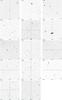 |
Fig. 2 Finding charts for the 14 targets of this study: B0007+106, B0109+224, B0405-123, B0716+714, B0823-223, B0955+326, B1101-325, B1147+245, B1215+303, B1424+240, B1722+119, B2155-304, B2254+074, and B2300-683 from top to bottom and left to right. |
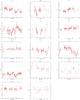 |
Fig. 3 R mag for the 14 targets of this study. |
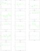 |
Fig. 4 V mag for the 14 targets of this study. |
Basic data about the targets used in this study.
5. Periodogram analysis
Magnitude variations shown in Figs. 3 and 4 are beyond the formal uncertainties given by the photometric reduction process (0.05 mag). There is also a strong correlation between the light curves obtained with the two filters, which convinces us that these variations are intrinsic to the studied objects. Alternatively, it can then be noted that the amplitude of the magnitude variations are in the range [ 0.05 / 2 ] during the time of our experiment.
Binary central compact objects are not part of the current unified model of AGN. Despite this, one could reasonably suspect that the rotation of the accretion disk and the dynamic of the accretion flow produce some periodic or quasi-periodic phenomena. It must be noted that supermassive binary black holes are predicted to be in an inevitable late stage in the evolution of the galaxy mergers (Beckmann & Shrader 2012). Recently, Graham et al. (2015) have reported the existence of a possible close supermassive binary black holes with subparsec separation in a quasar with optical periodicity of 1884+/−88 days.
Many objects are well known to exhibit one or more (quasi-)periodicity, such as B0109+224 (Ciprini et al. 2003), B0716+714 (Zhang, et al. 2009), B0735+178 (Qian & Tao 2004), and B1253-055 (Li et al. 2009). These four examples are sources coming from the ICRF, the first two are defining sources, and the last one has a variability period of about 130.6 days (radio, optical, and X-ray band) that could be explained by the helical motion of the jet.
This section presents two independent methods for analyzing the time series of magnitude obtained with the TAROT telescopes, the Lomb-Scargle periodogram, and the CLEAN algorithm.
5.1. Lomb-Scargle method
The Lomb-Scargle periodogram is a very common tool for spectral analysis of time series with unequally spaced data. It is equivalent to the least-squares fitting of a sine wave. We consider (Scargle 1982; Press & Rybicky 1989) a set of observations hi,i = 1,...,N obtained at times ti. The mean and variance of the observations are respectively defined by  (1)We assume that there are M test frequencies f1,f2,...,fM and their corresponding angular frequencies ω1,ω2,...,ωM, for j = 1,2,...,M. For each angular frequency ωj = 2πfj> 0 of interest, the time offset τ is given by
  (2)The Lomb-Scargle normalized periodogram (spectral power as a function of ω) is defined by
 ![\begin{eqnarray} P(\omega_{j})&=&\dfrac{1}{2\sigma^{2}}.\left\{\dfrac{\left[\sum_i (h_{i}-\tilde{h}).\cos\omega_{j}(t_{i}-\tau)\right]^{2} }{\sum_i \cos^{2} \omega_{j}(t_{i}-\tau)}\nonumber\right.\\ &&\left.\quad+\dfrac{\left[\sum_i(h_{i}-\tilde{h}).\sin\omega_{j}(t_{i}-\tau)\right]^{2}}{\sum_i \sin^{2}\omega_{j}(t_{i}-\tau)}\right\}\cdot \end{eqnarray}](/articles/aa/full_html/2016/03/aa26676-15/aa26676-15-eq48.png) (3)The probality p of observing a power less than or equal to P0 is given by
(3)The probality p of observing a power less than or equal to P0 is given by  (4)and the probability of seeing at least one sample exceeding this value by
  (5)The periodogram is calculated for frequencies ωj = 2πj/T,j = 1,...,M, where T is the total time interval covered by the data. This method has been applied to the previously mentioned targets B1253-055 (Li et al. 2009), B0735+178 (Qian & Tao 2004) and B0109+224 (Ciprini et al. 2003) and allows finding some (quasi-)periodic phenomena.
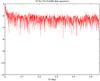 |
Fig. 5 Dirty spectrum for B0716+714 obtained with the CLEAN algorithm. |
5.2. CLEAN algorithm
An independent method was chosen to confirm the frequencies obtained by the Lomb-Scargle method (to avoid misinterpretation of frequency peaks). This method, the CLEAN algorithm, has been described by Roberts et al. (1987) and, in our case, implemented by (Jablonski, priv. comm.). It is the one-dimensional version of a cleaning algorithm developed for aperture synthesis in radioastronomy (Hogbom 1974). The CLEAN technique was developed as an attempt to remove alias frequencies from the periodogram. The first step of the method is to compute the so-called dirty spectrum. It is the discrete Fourier transform of the sampled signal or the convolution product of the Fourier transform of the signal by the window function. It can be written as 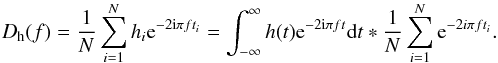 (6)In the case of IERS B0716+714, Fig. 5 illustrates the dirty spectrum as the first step in the iteration process in the CLEAN algorithm. The CLEAN algorithm is then an iterative process, and in the first step, the strongest line of the dirty spectrum is identified and the corresponding amplitude is multiplied by a gain factor g. This gives the first component of an intermediate “clean” spectrum. The g factor is needed because an error can occur when one frequency is determined in the presence of several periodic signals. Only a fraction g of this period is removed in one iteration step, so the error is reduced in proceeding iteration. A g factor of 0.1 means that ten iterations are needed to clean one frequency. The previously determined frequency is then removed from the dirty spectrum to form the first residual spectrum. The second iteration is then performed to find the strongest line in the first residual spectrum. This iteration process is repeated until a stopping condition is reached. The “clean” spectrum is then convolved with a Gaussian and added to the final residual spectrum to give the desired CLEAN periodogram.
6. Periodogram analysis of the observational data
In this section we present the analysis of the light curves obtained during four years, as presented in section four. Figures A.1 to A.4 present the periodograms obtained with the Lomb-Scargle method and with the CLEAN algorithm. The y-axis is the power spectrum as a function of the frequency f, given on the x-axis in units of day-1. For the Lomb-Scargle method, these confidence levels are 90%, 95%, 99%, 99.5%, 99.9%, and they are plotted as horizontal bars. Concerning the CLEAN algorithm, we chose the value 90% for comparison purposes. (The frequencies below this value are not represented.)
Tables 2 and 3 give a summary of the periods obtained with the two periodogram analyses in the R and V-bands, respectively. Only the periods that are common to both algorithms are retained in this table. By common we mean the nearest periods obtained by both of them. We have not retained those periods that are found only by one or the other of the algorithms. We note that the resulting difference never exceeds 7.9% in the R-band and 6.8% in the V-band. Both Tables 2 and 3 indicate that there is no correlation between the confidence level of the Lomb-Scargle method (Col. 3) and the relative difference of the periods given by the two methods (Col. 5). In other words, when the confidence level is low (90%), the relative difference in the periods does not seem worse than in the case of a high confidence level (99.9%). Table 4 summarizes the comparison of the periods obtained by the two methods in the two filters. For both filters, the period given in that table is the average of the periods given in Tables 2 and 3. Roughly two-thirds of the periods are common (difference lower than 10%) to both filters. This proportion could be explained by the fact that the number of observations is not exactly the same between the two filters. Physical phenomena could also explained such a ratio; nevertheless, the wavelength of the filters are very close, and it seems difficult to draw a conclusion in this way. Some periods obtained in this study, for the well-observed BL Lacertae object B0716+714, are already known. A period of 68 days is mentioned by Katajainen et al. (2000), and a period of three years is mentioned by Raiteri et al. (2003). For the BL Lac object B1215+303, two periods of 4.45 and 6.89 yr are mentioned by Fan et al. (2002). The first one is in good agreement (10%) with one of our results. For B0109+224, Ciprini et al. (2003) mentioned periods of about 25−40 days and 1.2 yr, so close in correlation with our results. Sandrinelli et al. (2014) find quasi-periodicities for the BL Lacertae object B2155-304. A peak of the Fourier spectrum is found with high significance at 315 days, which is also in good agreement with our result.
Comparison between the periods determined by the Lomb-Scargle and CLEAN algorithms in the R-band.
Comparison between the periods determined by the Lomb-Scargle and CLEAN algorithms in the V-band.
7. Structure functions
The structure function (SF) is a statistical tool that allows characterizing the variability of our targets. It quantifies the variability amplitude as a function of the time lag. The SF is commonly characterized in terms of its slope α, where SF(τ) ≈ τα. This work of reference was done by Rutman (1978) where the author wanted to characterize the phase and frequency instabilities in precision frequency sources. This work was mostly dedicated to characterizing the phase (or frequency) stability of atomic clocks (or atomic time scales). The first application of the SF to the study of extragalactic sources was made by Simonetti et al. (1985). For a finite sequence of measurements f(i),i = 1,...,N, the first order SF is estimated by 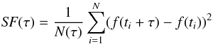 (7)where τ is the separation time of the observations.
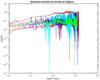 |
Fig. 6 Structure function for the BL Lac objects. The curves of the objects 1722+119, 2155-304 and 2254+074 are in blue, cyan, and green, respectively. |
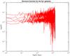 |
Fig. 7 Structure function for the Sy1 objects |
The total number of data pairs that can be constructed for N epochs is N(N − 1) / 2. For this work they were grouped and averaged into time spans of one day.
The slope α of the structure function in a log (SF) − log (τ) diagram characterizes the variability, hence the underlying process. If α = 1, shot noise dominates, toward flatter slopes (α = 0) where flicker noise becomes more important. When a light curve contains a periodic signal, the structure function rises to a maximum at half the period and then falls to a minimum for the period of the signal (Smith et al. 1993).
Figures 6 and 7 present the structure functions for the BL Lac and the Sy1 objects, respectively. In the first set of objects, all but three, have a structure function with a slope ~0.39 before 100 days and ~0 after. In this first set, the objects 1722+119, 2155-304, and 2254+074 have a structure function with a slope ~0 at all τ. This is exactly the behavior of the second set of objects (the Seyfert galaxies), where the slope is ~0 at all τ. The complete SF, for the two sets of objects, can then be modeled by broken power-law models.
Even though the SF is is an extensively used tool in the field of AGN variability, some problems could occur as emphasized by Emmanoulopoulos et al. (2010). The authors show that the SF results are sometimes erroneously interpreted, leading to misconceptions about the actual source properties. The lack of statistical independence between adjacent SF points means that it is not possible to perform robust statistical model fitting following the commonly used least-squares fitting methodology. The positions of breaks and slopes are always much less than the actual scatter of these variables. SFs are also severely troubled by gaps that can induce artifacts and systematic deviations.
8. Conclusion and prospects
The number of observations and their sampling makes our set of data one of the largest databases in the optical wavelength, for some AGNs suitable for the link between the reference frames.
These data can also be very useful for astrophysics and can be used both for short- or long-term studies. As a matter of example, some objects (SDSS J121855.80+020002.1 and SDSSJ162011.28+172427.5) could be good candidates for a binary black hole system (Popovic et al. 2012), and they sometimes exhibit light curves (PG1302-102) that could be explained by the presence of two supermessive black holes with subparsec separation (Graham et al. 2015). Nevertheless, in the latter case, we also recall that orbital periods of a few years imply orbits so close that the two BH orbit inside the accretion disk. Our analysis showed that periodic or quasi-periodic phenomena are present for all but one target. The periods go from some days to some years and involve different kinds of astrophysical phenomena. For four objects, the periods determined in the frame of this study are in very good agreement with those periods that are already known. Apart for these four objects, the periodicities for the other ones were unknown. They were determined by two different methods, and they agree in both cases.
Comparison between the periods determined by the two methods in the R and V-bands.
List of observations from 2011 to 2015 in the R filter.
List of observations from 2011 to 2015 in the V filter.
Structure functions were computed for the two sets of objects (BL Lac and Sy1) and show good agreement between the results in each group, except for three of them. For these three particular cases, the objects of interest (BL Lac) have structure functions that are more similar to the ones of the Sy1 set of objects. Even though the structure function is a very well known and used tool in the field of the AGN variability, it would be used with care because its results are sometimes erroneously interpreted.
All the observed objects for this study are highly variable sources in the R and V-bands (either Seyfert galaxies or BL Lac objects). The underlying astrophysical phenomena could displace the photocenter of the targets. In the case of an object with a deterministic behavior, an astrophysical model, if it exists, can give information about the signature of the photometric variations. In contrast, the photometric variations can bring constraints on astrophysical models that are parametrized by the distance between the radiocenter and the photocenter. This distance must be taken into account for the link of the reference systems. If the photocenter flicker could not be modeled, an uncertainty, that takes it into account in a conservative way, must be considered when using the optical astrometric position for the link of the reference frames. In the other cases (no astrophysical models, no astrometric uncertainty due to flickering), the considered targets would not be suitable for the link between reference systems. Popovic et al. (2012) have studied the photocenter position variability caused by variations in the quasar inner structure (accretion disk emissivity, torus structure variability, exploding stars very close to the AGN source and binary supermassive black hole). They conclude that variations in the quasar inner structure can affect the observed photocenter by up to several mas.
Moreover it was recalled that the position of radio sources as measured by geodetic VLBI shows displacements larger than 0.1 mas in rms, essentially owing to instrumental or atmospheric limitations. If the nucleus of the radio quasar contains an active BBH system, then the astrometric precision will be obviously limited by the size of this system. Finally it is known that photometric variabilty can occur on time scales longer than our observation time span (Smith et al. 1993). These very long photometric variations could be due to the larger regions (dust torus, host galaxy) and could have an impact at the level of some mas on the astrometry of the targets.
Other optical observations are currently in progress to monitor the magnitude of 47 weak extragalactic radio sources (12 BL Lac objects and 35 quasars) with bright optical counterparts (Bourda et al. 2011), which come from the CLASS catalog (Myers et al. 2003). They were chosen because only 70% of the sources coming from the ICRF are suitable to establishing the link with the future Gaia Reference Frame. These targets are observed in the optical wavelength with the 0.8 m-TJO9 (Telescopi Joan Oro), a robotic telescope oparated by the Institut d’Estudis Espacials de Catalunya (IEEC). The first results of this observing campaign will be published elsewhere, together with the study of the objects coming from the quasars group published by Bourda et al. (2008).
References
- Beckmann, V., Shrader, C. 2012, in Active Galactic Nuclei, Wiley-VCH Verlag GmbH & Co. [Google Scholar]
- Bertin, E., & Arnouts, S. 1996, A&AS, 117, 393 [NASA ADS] [CrossRef] [EDP Sciences] [Google Scholar]
- Britzen, S., Roland, J., Laskar, J., et al. 2001, A&A, 374, 784 [Google Scholar]
- Bourda, G., Charlot, P., & Le Campion, J. 2008, A&A, 490, 403 [NASA ADS] [CrossRef] [EDP Sciences] [Google Scholar]
- Bourda, G., Collioud, A., Charlot, P., et al. 2011, A&A, 526, A102 [NASA ADS] [CrossRef] [EDP Sciences] [Google Scholar]
- Ciprini, S., Tosti, G., Raiteri, C., et al. 2003, A&A, 400, 487 [NASA ADS] [CrossRef] [EDP Sciences] [Google Scholar]
- Damerdji, Y., Klotz, A., & Boër, M. 2007, AJ, 133, 1470 [NASA ADS] [CrossRef] [Google Scholar]
- de Bruijne, J. H. J. 2012, Ap&SS, 341, 31 [NASA ADS] [CrossRef] [Google Scholar]
- Emmanoulopoulos, D., McHardy, I., & Uttley, P. 2010, MNRAS, 404, 931 [NASA ADS] [CrossRef] [Google Scholar]
- Fan, J., Lin, R., Xie, G., et al. 2002, A&A, 381, 1 [NASA ADS] [CrossRef] [EDP Sciences] [Google Scholar]
- Fey, A. L., Ma, C., Arias, E. F., et al. 2004, AJ, 127, 3587 [NASA ADS] [CrossRef] [Google Scholar]
- Fey, A. L., Gordon, D. G., & Jacobs, C. S. 2009, IERS Technical Note 35 [Google Scholar]
- Graham, M., Djorgovski, S., Stern, D., et al. 2015, Nature, 518, 74 [NASA ADS] [CrossRef] [Google Scholar]
- Hogbom, J. 1974, A&AS, 15, 417 [NASA ADS] [Google Scholar]
- Katajainen, S., Takalo, L., & Sillanpaa, A. 2000, A&AS, 143, 357 [NASA ADS] [CrossRef] [EDP Sciences] [Google Scholar]
- Klotz, A., Boër, M., Eysseric, J., et al. 2008, PASP, 120, 1298 [NASA ADS] [CrossRef] [Google Scholar]
- Li, H., Xie, G., & Chen, L., et al. 2009, PASP, 121, 1172 [NASA ADS] [CrossRef] [Google Scholar]
- Lobanov, A., & Roland, J. 2005, A&A, 431, 831 [NASA ADS] [CrossRef] [EDP Sciences] [Google Scholar]
- Ma, C., Arias, E. F., Eubanks, T. M., et al. 1998, AJ, 116, 516 [NASA ADS] [CrossRef] [Google Scholar]
- Mignard, F. 2002, EAS Pub. Ser., 2, 327 [Google Scholar]
- Myers, S., Jackson, N., Browne, I., et al. 2003, MNRAS, 341, 1 [NASA ADS] [CrossRef] [Google Scholar]
- Pelletier, G., & Roland, J. 1989, A&A, 224, 24 [NASA ADS] [Google Scholar]
- Pelletier, G., & Roland, J. 1990, in Parsec-scale radio jets, eds. J. Zensus, & T. Pearson (Cambridge University Press), 323 [Google Scholar]
- Pelletier, G., & Sol, H. 1992, MNRAS, 254, 635 [NASA ADS] [Google Scholar]
- Popovic, L., Jovanovic, P., Stavlevski, M., et al. 2012, A&A, 538, A107 [NASA ADS] [CrossRef] [EDP Sciences] [Google Scholar]
- Press, W., & Rybicki, G. 1989, ApJ, 338, 277 [NASA ADS] [CrossRef] [Google Scholar]
- Qian, B., & Tao, J. 2004, PASP, 116, 161 [NASA ADS] [CrossRef] [Google Scholar]
- Raiteri, C., Villata, M., Tosti, G., et al. 2003, A&A, 402, 151 [NASA ADS] [CrossRef] [EDP Sciences] [Google Scholar]
- Roberts, D. H., Lehar, J., & Dreher, J. W. 1987, AJ, 93, 968 [NASA ADS] [CrossRef] [Google Scholar]
- Roland, J. 2014, in Journée 2013 Systèmes de référence spatio-temporels, ed. N. Capitaine, 28 [Google Scholar]
- Roland, J., Britzen, Kudryavtseva, N., et al. 2008, A&A, 483, 125 [NASA ADS] [CrossRef] [EDP Sciences] [Google Scholar]
- Roland, J., Britzen, Witzel, A., & Zensus, J. 2009, A&A, 496, 645 [NASA ADS] [CrossRef] [EDP Sciences] [Google Scholar]
- Roland, J., Britzen, S., Caproni, A., et al. 2013, A&A, 557, A85 [Google Scholar]
- Roland, J., Britzen, Kun, E., et al. 2015, A&A, 578, A86 [NASA ADS] [CrossRef] [EDP Sciences] [Google Scholar]
- Rutman, J. 1978, Proc. IEEE, 66, 9, 1048 [NASA ADS] [CrossRef] [Google Scholar]
- Sandrinelli, A., Covino, S., & Treves, A. 2014, ApJ, 793, L1 [NASA ADS] [CrossRef] [Google Scholar]
- Scargle, J. D. 1982, ApJ, 263, 835 [NASA ADS] [CrossRef] [Google Scholar]
- Simonetti, J., Cordes, J., & Heeschen, D. 1985, ApJ, 296, 46 [NASA ADS] [CrossRef] [Google Scholar]
- Smith, A., Nair, A., Leacock, R., et al. 1993, AJ, 105, 437 [NASA ADS] [CrossRef] [Google Scholar]
- Sol, H., Pelletier, G., & Asseo, E. 1989, MNRAS, 237, 411 [NASA ADS] [Google Scholar]
- Souchay, J., Andrei, A., Barache, C., et al. 2012, A&A, 537, A99 [NASA ADS] [CrossRef] [EDP Sciences] [Google Scholar]
- Taris, F., Andrei, A., Klotz, A., et al. 2013, A&A, 552, A98 [NASA ADS] [CrossRef] [EDP Sciences] [Google Scholar]
- Zhang, H., Zhang, X., Dong, F., et al. 2009, Chin. Astron. Astrophys., 33, 373 [NASA ADS] [CrossRef] [Google Scholar]
Appendix A: Additional figures
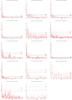 |
Fig. A.1 Lomb Scargle periodograms in R-band. The horizontal lines correspond to the confidence levels, 90%, 95%, 99%, 99.5% and 99.9% (from bottom to top). |
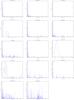 |
Fig. A.2 CLEAN periodograms in R-band (frenquencies with more than a 90% confidence level). |
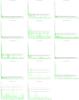 |
Fig. A.3 Lomb Scargle periodograms in V-band. The horizontal lines correspond to the confidence levels 90%, 95%, 99%, 99.5%, and 99.9% (from bottom to top). |
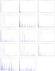 |
Fig. A.4 CLEAN periodograms in V-band (frenquencies with more than 90% of confidence level). |
All Tables
Comparison between the periods determined by the Lomb-Scargle and CLEAN algorithms in the R-band.
Comparison between the periods determined by the Lomb-Scargle and CLEAN algorithms in the V-band.
Comparison between the periods determined by the two methods in the R and V-bands.
All Figures
|
Fig. 1 Rms of the coordinate time series of the most observed quasars in the geodetic VLBI monitoring program of the International VLBI Service for Geodesy and Astrometry (IVS; Lambert, priv. comm.) as a function of the number of sessions. |
| In the text | |
|
Fig. 2 Finding charts for the 14 targets of this study: B0007+106, B0109+224, B0405-123, B0716+714, B0823-223, B0955+326, B1101-325, B1147+245, B1215+303, B1424+240, B1722+119, B2155-304, B2254+074, and B2300-683 from top to bottom and left to right. |
| In the text | |
|
Fig. 3 R mag for the 14 targets of this study. |
| In the text | |
|
Fig. 4 V mag for the 14 targets of this study. |
| In the text | |
|
Fig. 5 Dirty spectrum for B0716+714 obtained with the CLEAN algorithm. |
| In the text | |
|
Fig. 6 Structure function for the BL Lac objects. The curves of the objects 1722+119, 2155-304 and 2254+074 are in blue, cyan, and green, respectively. |
| In the text | |
|
Fig. 7 Structure function for the Sy1 objects |
| In the text | |
|
Fig. A.1 Lomb Scargle periodograms in R-band. The horizontal lines correspond to the confidence levels, 90%, 95%, 99%, 99.5% and 99.9% (from bottom to top). |
| In the text | |
|
Fig. A.2 CLEAN periodograms in R-band (frenquencies with more than a 90% confidence level). |
| In the text | |
|
Fig. A.3 Lomb Scargle periodograms in V-band. The horizontal lines correspond to the confidence levels 90%, 95%, 99%, 99.5%, and 99.9% (from bottom to top). |
| In the text | |
|
Fig. A.4 CLEAN periodograms in V-band (frenquencies with more than 90% of confidence level). |
| In the text | |
Current usage metrics show cumulative count of Article Views (full-text article views including HTML views, PDF and ePub downloads, according to the available data) and Abstracts Views on Vision4Press platform.
Data correspond to usage on the plateform after 2015. The current usage metrics is available 48-96 hours after online publication and is updated daily on week days.
Initial download of the metrics may take a while.