| Issue |
A&A
Volume 586, February 2016
|
|
|---|---|---|
| Article Number | A2 | |
| Number of page(s) | 10 | |
| Section | Extragalactic astronomy | |
| DOI | https://doi.org/10.1051/0004-6361/201527047 | |
| Published online | 19 January 2016 | |
Probing the photoionised outflow in the NLS1 Arakelian 564: An XMM-Newton view
1 Leiden Observatory, Leiden University, PO Box 9513, 2300 RA Leiden, The Netherlands
e-mail: khanna@strw.leidenuniv.nl
2 SRON Netherlands Institute for Space Research, Sorbonnelaan 2, 3584 CA Utrecht, The Netherlands
3 Department of Physics and Astronomy, Universiteit Utrecht, PO Box 80000, 3508 TA Utrecht, The Netherlands
Received: 24 July 2015
Accepted: 8 November 2015
We present a detailed analysis of XMM-Newton X-ray observations of the narrow-line Seyfert-1 (NLS1) galaxy Ark 564, taken between 2000 and 2011. High-resolution X-ray spectroscopy was carried out on the resultant high signal-to-noise stacked spectrum. We find three separate photoionised warm absorbers, which outflow at velocities unusually lower than typical NLS1s. Using recombination timescale estimates, improved constraints on the location of these clouds show they could be located beyond 4 pc from the central source. Our estimates of the outflow kinetics suggest that the active galactic nucleus in Ark 564 is unlikely to affect the host galaxy in its current state, but over a typical lifetime of 107 yr the interstellar medium could be affected. The individual observations used here suggest the luminosity varies over weekly timescales and, in addition, we find evidence of gas response to changes in the ionising radiation.
Key words: galaxies: active / galaxies: nuclei / galaxies: Seyfert / galaxies: individual: Ark 564 / X-rays: galaxies
© ESO, 2016
1. Introduction
Active galactic nuclei (AGN) are among the brightest objects in the sky, spanning across nine orders of magnitude in luminosity (Shang et al. 2011). The engine of this energy output is thought to be accretion onto a supermassive black hole (SMBH) at the centre of the host galaxy, which results in typical luminosities of ~1042 erg s-1 (Seyferts) to 1046 erg s-1 (Quasars). In addition to a bright continuum, a plethora of absorption and emission features in the X-ray band are also a common feature and, in several sources, the observed spectral lines are blue-shifted by several 1000 km s-1, which indicates the presence of outflowing gas in the line of sight. One suggested explanation is that these outflows are produced by irradiation of the dusty gas torus structure (Antonucci 1993), which surrounds the SMBH and accretion disk (Krolik & Kriss 2001).
High resolution X-ray spectroscopy can be performed on nearby sources and this allows us to characterize both the environment as well as the energetics associated with ionised outflows from AGN. This is important in the context of feedback to the host galaxy, which is considered a solution to the galaxy luminosity function bright-end problem (Silk & Mamon 2012). But since only about 10% of AGN are radio-loud (Calafut & Wiita 2015), it seems natural to consider the kinetics of the radio-quiet sources, such as Seyferts, which are a sub-class of AGN found in the nearby universe. While in Seyfert 2 galaxies, both the disk and black hole are obscured by dust (side-on view), in Seyfert 1’s, both these features are visible (top-down view) making them ideal candidates for studying outflows. In particular narrow-line Seyfert-1s (NLS1s) show broad absorption troughs in the optical and X-ray and also exhibit strong Fe (II) lines (Osterbrock & Pogge 1985), which allows regions close to the central source to be studied. In many low-luminosity Seyfert galaxies, partially ionised material or “warm-absorbers” gives rise to absorption features at energies around 1 keV. In the last two decades, surveys have found warm-absorption in about 50% of nearby Seyferts (Nandra & Pounds 1994; Blustin et al. 2005). In recent years, warm-absorbers have also been detected in a few radio galaxies, although the jet still remains the dominant feedback mechanisms in this type of AGN (Torresi et al. 2012).
In this paper, we attempt to characterise the physical structure of the NLS1 AGN Arakelian 564 (hereafter Ark 564) by making use of all XMM-Newton data on the source so far. Ark 564 is located at a redshift z = 0.02468 and is among the brightest sources in the nearby universe with a 2−10 keV flux f2−10 ~ 10-11 erg s-1 cm-2. We perform spectral analysis on the stacked spectrum to determine the ionisation and dynamical structure of the outflow. Ark 564, like several other NLS1s, is already known to be a highly variable source, best illustrated during the month-long ASCA observation by Gliozzi et al. (2002), when it displayed non-linear behaviour. Given the timespan of our data, we look for long-term variability of the source and the resulting gas response.
Radio-quiet quasars are scaled up versions of Seyferts (Leipski et al. 2006) that are found at cosmological distances (z> 0.1). Estimating the mass loss in nearby AGN can provide order-of-magnitude estimates of the impact of outflows on host galaxy star-formation (Krongold et al. 2007). We derive similar quantities and compare them with other well-known sources.
2. Observations and data reduction
The data were extracted using the XMM-Newton SAS software v13.5. Fluxed spectra with 0.01 Å-wide bins were created for each RGS detector and each spectral order, and for each individual observation. Following the methods described by Kaastra et al. (2011), the four spectra were combined into one spectrum using the RGS_fluxcombine program, an auxiliary program of the spex software (Kaastra et al. 1996) version 2.06.001. The same program is used to produce the stacked total spectrum of Ark 564, and the optimised response matrices were produced using the RGS_fmat program. The details of the 13 XMM-Newton RGS observations are provided in Table 1. The average exposure time is about 50 ks. To obtain the best signal-to-noise ratio (S/N), the individual observations have been stacked together to produce a time-averaged spectrum, as discussed in Sect. 3.2.
Details of the XMM-Newton (RGS) observations of Ark 564.
3. Spectral analysis
3.1. Source spectral energy distribution
For the purpose of photoionisation modelling of the outflows, we determined the broadband spectral energy distribution (SED) of the ionising source in Ark 564 (Fig. 1). The UV and X-ray parts of the SED were constructed from the XMM-Newton OM photometric filters (UVW1, UVM2, and UVW2) and the EPIC-pn spectrum (0.3–10 keV).
To expand the energy coverage of the SED beyond that of XMM-Newton into lower and higher energies, we used archival flux measurements from the NASA/IPAC Extragalactic Database (NED). We extracted infrared flux measurements at 25, 60, and 100 micron from IRAS and a radio flux measurement at 2380 MHz from Arecibo. We also included a Suzaku flux measurement given over the 10–50 keV band. As the source becomes too faint at hard X-rays, we applied a cut-off at 400 keV to our continuum model, which is a typical cut-off value found in bright AGN, e.g. NGC 5548 (Ursini et al. 2015).
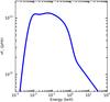 |
Fig. 1 Spectral energy distribution of Ark 564, derived using the EPIC-pn and OM data of 2011 XMM-Newton observations. |
We determined the SED by applying a broadband AGN continuum model to the above data. We used the broadband continuum model discussed in Mehdipour et al. (2011, 2015), which is based on Compton up-scattering of the IR/optical/UV disk photons to X-ray energies in warm and hot coronae. The use of this model enables us to establish the continuum from infrared to X-ray energies, including the extreme-UV part, which is important for photoionisation calculations.
In addition to correcting for interstellar X-ray absorption and reddening in the Galaxy, we also corrected for reddening in the host galaxy of Ark 564. There are reports of substantial internal reddening in Ark 564. Thus, we adopted the colour excess E(B−V) = 0.14 reported by Crenshaw et al. (2002) to correct for host galaxy reddening in Ark 564, assuming the same dust extinction law as the Galaxy. In our Galaxy, the colour excess is smaller at E(B−V) = 0.03 (Schlegel et al. 1998). To correct the data, we applied the reddening curve of Cardelli et al. (1989), including the update for near-UV given by O’Donnell (1994).
All spectra were modelled using the spex code, adopting a Λ-cosmology with ΩΛ = 0.7, ΩM = 0.3, and H0 = 70 km s-1 Mpc-1. For the spectral analysis we use χ2 statistics and the optimum data bin size was determined using Shannon binning. Adopting this the data were binned with a redistribution function FWHM of △E/3. The RGS resolution is 70 mÅ (Shannon FWHM ~ 50 points/Å), while our stacked spectrum has 100 points/Å. We have thus binned our data by a factor of two.
3.2. Continuum fitting
In previous studies, the continuum has usually been modelled with a steep power law of photon index ~2.5 and soft blackbody components (Vignali et al. 2004). But others have also shown that the soft part is not very well modelled with a simple blackbody, and there have been relativistic disk profiles as well as multiple blackbody components in one fit (Papadakis et al. 2007). Taking a cautious approach we use spline interpolation to fit the basic continuum. A grid of 18 points that are equally spaced by 2 Å was used over the range 6−40 Å with an extended boundary to reduce errors caused by sharp discontinuity at the edge of the RGS band.
For the Galactic interstellar X-ray absorption we used the spex HOT model with NH = 5.34 × 1020 cm-2 in our line of sight towards Ark 564 (Kalberla et al. 2005). This is assumed to be a cold neutral absorber (kT ~ 0.5 eV) and clearly fits the O I Galactic oxygen line at 23.5 Å in the RGS spectrum. This was also identified earlier by Ramírez (2013) and Smith et al. (2008). However, the HOT model also predicts absorption around 17.47 Å, which corresponds to neutral iron. The data do not show a strong signature here and this is likely due to Galactic dust. By freeing the atomic Fe abundance in the hot model and including iron in dust form (using the amol model in spex and component Fe2O3) we get a much better fit (see the blue line in Fig. 2) with an Fe2O3 column of NH = 3.36 × 1015 cm-2. This is consistent with other high-resolution X-ray spectra through the Galactic interstellar medium (ISM), e.g. Pinto et al. (2013). It is not unlikely that the Galactic foreground medium has multiple temperature components and, indeed, we also notice O VII absorption at 21.6 Å, which is well-fitted with a second warmer HOT model with a temperature ~0.15 keV and turbulence with vturb = 36 ± 20 km s-1. This is the 1s2 g1S0−1s2p 1P1 transition (Mewe et al. 1985).
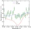 |
Fig. 2 Weakness of galactic neutral iron in gas form (red curve) in the line of sight to Ark 564 predicted by NH = 5.34 × 1020 cm-2 (Kalberla et al. 2005), suggesting the presence of Fe in dust form (blue curve) in our own Galaxy. |
3.3. Emission lines
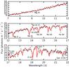 |
Fig. 3 Blow-up of the high resolution RGS spectrum of Ark 564 showing important emission and absorption lines between 7−22 Å, as discussed in the text. The best-fit final full spectrum (7−38 Å) with residuals is shown in Fig. 5. |
Figures 3 and 4 show zoomed-in sections of the main spectrum, highlighting the emission features. These were fitted with the DELTA and VGAU models in spex, which incorporate narrow emission lines with Gaussian broadening. Prominent lines are listed in Table 2, along with the broadening velocity σ.
Narrow and broad non-relativistic emission lines with line flux as observed.
We infer three distinct zones from which the emission lines could originate. The Lyα lines for C, N, and O seem to be from a high-velocity/turbulence zone, while the two forbidden lines (O VII and Ne IX) show a negligible outflow signature. In addition, the intercombination line of N VI is half as broadened as that of the Lyα lines. Smith et al. (2008) suggest that since signature of intercombination lines is an indication of high density and, since the N VI(i) and O VII(f) and Ne IX(f) seem to come from separate components, this suggests that the faster component could also be denser. However, we note that for oxygen the derived density estimates from line ratios is probably unreliable owing to self-absorption of the resonance and then the intercombination line (Mehdipour et al. 2015).
The narrow and broad emission lines are generally assumed to arise from a photoionized plasma where, in general, the temperature is much lower than the ionisation potential of the dominant ions in the plasma. In this case, we expect to see radiative recombination continua (RRC). Candidates for RRC in our band include O VII, C V, and Ne IX. While we do not detect carbon or neon RRC, there is clearly a feature around 17 Å which corresponds to the O VIII to O VII recombination. In addition we find a Doppler shift ( ) at the source for this feature of zDop = −2.43 × 10⁻³, which corresponds to a blueshift of about 800 km s-1.
3.4. Relativistic broad lines?
From the stacked spectrum two extremely broad asymmetric features seem apparent in the region covering 18–30 Å. We explore the possibility of these being broad relativistic emission lines that originate from the O VIII and N VII Lyman alpha transitions. Relativistically broadened skewed lines result from a combination of gravitational redshift that is due to the deep potential around black holes and relativistic beaming due to gas swirling at relativistic velocities (Fabian et al. 2002). There have been previous reports of broad Lyα lines for other sources such as MCG-6-30-15 and Mrk 766 (Branduardi-Raymont et al. 2001). We checked this broadened feature in the Ark 564 spectrum by modelling it with a LAOR profile (Laor 1991) in spex. The best fit results for an inner radius of 10 , consistent with a non-rotating black hole, with the disk aligned at about 37°. The parameters are provided in Table 3 and, by including the possible broad relativistic lines at the energies of O VIII and N VII Lyα, we improve Δχ2 ~ 500 for 1490 d.o.f. Figure 6 shows the spline continuum with and without the two relativistic lines and, although it would appear that the features are statistically significant (given the small error bars), we would like to point out that with a slightly higher, more power law-like spline continuum in this band, the remaining residuals are of the order of a few percent. Recent calibration work by one of us (J.S.K.) shows that the RGS effective area has remaining residuals at a similar level of a few percent on scales of a few Å. We leave it open here as to whether the relativistic lines are real or serve to compensate for small calibration uncertainties.
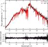 |
Fig. 5 Sstacked XMM-Newton RGS high-resolution spectrum produced by combining all Ark 564 RGS observations to date (in black). The final best fit (in red) consists of galactic absorption, broad and narrow Gaussian emission lines, three phases of photoionized warm-absorbers, all on a continuum modelled by spline interpolation. Lower panel: residuals (black) for this fit. |
Summary of the spectral features (other than narrow emission lines) and best-fit parameters used to model the stacked spectrum of Ark 564, resulting in a final χ2/ d.o.f. = 5178/3034.
Three warm absorber components found in Ark 564.
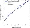 |
Fig. 6 Spline continuum with fitting for broad relativistic lines. The error bars are insignificant as is illustrated in the blow-up of the relevant region: N VII (24.73 Å) and O VIII (18.94 Å) in the laboratory frame. |
3.5. Photoionisation modelling of absorption clouds
A preliminary search for absorption features was performed using the SLAB model (Kaastra et al. 2002) in spex, which allows for ionic column densities to be chosen independently. This also provided an estimate of the outflow velocity of the absorbing gas. For a more realistic calculation we made use of XABS components in spex. The XABS model calculates the transmission of a slab of material, where all ionic column densities are linked through the CLOUDY (Ferland et al. 1998) photoionisation model. The parameters fitted for each XABS component are the ionisation parameter ( ), turbulence, outflow velocity, and the column density with n(R) defined as the hydrogen gas density at R which is the distance between the source and the absorber. We made use of the derived SED of Ark 564 (Sect. 3.1) to calculate the ionisation balance in the CLOUDY code and obtain Lion = 6.9 × 1037 W. Here we assume Solar abundances (Lodders et al. 2009) however, since AGN are typically known to have high abundances in the elements C, N, O, and Fe (Komossa & Mathur 2001), we also tested for non-solar abundances but did not find strong deviations from solar metal abundance ratios, as found in the case of Mrk 509 by Steenbrugge et al. (2011). Hence, we have assumed Solar abundances for Ark 564. We find that the best fit is achieved with three separate XABS components with an equal spatial covering factor fcov = 1. These vary in ionisation as well as in their outflow signature. Table 4 ranks the three absorption phases identified by their ionisation parameter (ξ) and, additionally, we note that the highly ionized Phase 3 produces most of the Fe and Ne lines. Compared with the outflow velocities for emission lines in Table 2, the absorbing gas seems to be present in weakly outflowing regions, which suggests that the origin of the absorber and the emission lines is likely to be different. However, the OVII(f) does have broadening comparable to Phases 2 and 3, so there could be a connection between these.
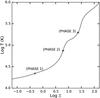 |
Fig. 7 Stability curve with the positions indicated of the three warm absorbers from our best fit for Ark 564. The absence of a region with negative slope on the S-curve indicates there are no unstable regions i.e. gas can exist in equilibrium throughout the curve. This is likely due to the steep soft-excess seen in Ark 564, which allows gas to cool efficiently by lowering the Compton temperature. (Marker size exaggerated to show against small error bars in green.) |
On the basis of the distinct ξ parameters that we find, it would appear that Ark 564 has three separate absorption components. To test this further, in Fig. 7 we plot the pressure form of the ionisation parameter, Ξ = Lion/ 4πr2cnHkT against the absorber temperatures (≈105 K), derived using spex with the SED from the 2011 (Fig. 1) observations. In Fig. 7, regions with positive gradient represent where gas is in photo-ionisation equilibrium and is stable against thermal perturbations while the negative slopes indicate unstable zones. Since, at a given distance r, Lion is independent of gas density,  , and thus on such a plot, absorbers with a range of densities and temperatures can line up vertically if in pressure-equilibrium. This is considered to play a role in confining neighbouring outflowing clouds, such as in NGC 985, where the absorbers are present in a multi-phase wind (Krongold et al. 2005). For Ark 564, it is clear that the three absorbers do not line up on the stability curve and so are not in pressure equilibrium. We note that the kinetics of Phases 1 and 2 are very similar with regards to the outflow velocities, as compared to the negligible outflow in Phase 3. Additionally, there is overlap in the locations of the absorbers (Sect. 4.3) from Phases 1 and 2, so this perhaps suggests another mechanism by which these two zones are confined. Distinct ionisation components are also seen in other well studied sources. In NGC 5548 Steenbrugge et al. (2005) detect up to five components that are not in pressure equilibrium but display similar kinetics to each other, which points towards a single confined outflow, quite unlike our situation. Also, Mrk 509 (Ebrero et al. 2011) shows three distinct ionisation zones, although on the S-curve the outflowing components are in pressure equilibrium with each other, while the third component, which was in fact found to be redshifted, is not in equilibrium with its outflowing counterparts. For Ark 564, we also note that the S-curve does not have any unstable regions, which is likely due to the source having a steep soft X-ray spectrum that removes instabilities by lowering the Compton temperature of the gas, allowing it to cool more efficiently (Guilbert et al. 1983). Such behaviour has also been noted for other NLS1s, such as I ZW 1 (Costantini et al. 2007).
4. Discussion
4.1. Comparison with previous spectroscopic studies
The data sets used in this paper have been studied separately before. Generally the features we report are similar to other works. We obtain similar column density and ionisation parameters to Ramírez (2013), who observed Ark 564 using Chandra LETGS. The analysis of the line at observed wavelength of 19 Å suggests this is from Phase 2, and we get a slightly higher ionisation parameter of Log ξ = 1.34 to their Log ξ = 1.1, but very similar column density and line width. Smith et al. (2008) also show this line but do not discuss it. Giustini et al. (2015), using a different photoionisation code in xspec, find similar features to us.
Previous works mostly find the best-fit model to be consistent with two separate phases of warm absorbers. From the Ark 564 2005 observations, Papadakis et al. (2007) find two phases with Log ξ ~ 1 and 2, similar to the 2002 results from Matsumoto et al. (2004). Dewangan et al. (2007), using both EPIC and RGS data from 2005, report similar numbers and, in addition, find very high velocity outflows of up to 1000 km s-1. Smith et al. (2008) perform spectroscopy on the stacked spectrum of data up to 2005 and, although they assume continuum parameters as reported by Papadakis et al. (2007), they found the best-fit model requires three separate phases of absorption and not in pressure equilibrium, which is similar to the results presented in this paper.
4.2. Luminosity and Ionization variability
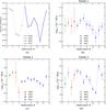 |
Fig. 8 a) Based on the best-fit parameters from the stacked spectrum we derive luminosities for all the individual observations between 2000−2011. The individual data sets are highlighted and so the combined plot is not evenly spaced in time. Observation # are as in Table 1. b), c) and d) Ionisation parameter (ξ) for the individual observations derived using stacked spectrum. Compared to a) it seems ξ varies in response to changing source luminosity. The response time is related to the gas density so the component in phase 3 is possibly denser than the remaining two warm-absorbers. |
The spectrum used in our analysis is compiled using 13 observations taken over a period of about 10 yr. Using the best-fit parameters from the high-resolution stacked spectrum, we can now look at the source during the individual observations. For each spectrum we are primarily interested in the gas response to changes in source luminosity, and so we keep all best-fit parameters from the stacked data frozen except for the normalisation of lines and continuum, as well as the ionisation parameter (ξ). The resulting set of parameters is shown in Table 5 and all spectra are fitted with χ2/ d.o.f. ~ 1.2. Based on this, in Fig. 8a we plot the long term light curve for Ark 564 where it is apparent that, over this period, the source seems to vary by a factor of two. Unlike continuous monitoring surveys, which allow analysis of evenly spaced time intervals, e.g. Gliozzi et al. (2002), here we have time-averaged observations taken over a decade. However, the 2011 data were taken every six days from May 2011 to July 2011 and so here we use this set to look for correlations. Additionally, we are interested in the gas response for which we use the ξ parameter as a proxy. Figures 8b−d show the variation in ionisation over all observations where, at first glance, it seems that during 2011 all three gas phases were responding to the ionizing luminosity. However, within the shown errors, only the highest ionized phase (# 3) seems to mirror the light curves in Fig. 8a, unlike the other two phases of warm absorbers.
We can use recombination timescales to estimate the location of the warm absorbers, i.e. the clouds of photoionized gas being radiatively driven out. Essentially, the response timescale to luminosity variations can be used as a measure for the gas density as  , such that denser gas should respond faster to changes in source luminosity (Reynolds & Fabian 1995). If the gas density is high enough then a rise in luminosity should be followed by a rise in ξ. This could be instantaneous (extremely dense) or there could be a significant lag (low density). In Figs. 8b−d we plot ξ for the individual observations, derived by using the best-fit parameters from the stacked spectrum as described earlier. The three panels show the gas response in each phase over the ten year period and visually it seems that the ionisation parameter was responding to the source luminosity during the 2011 campaign. To check this further in Fig. 9, we again plot the best-fit ξ parameter, but now against the ionising luminosity for all individual observations to search for correlations. We find that in all three phases there is a weak correlation with an average Pearson coefficient of ~0.45 and p-value ~10%, and so we cannot reject null hypothesis. However, if in 2011 (the evenly spaced data set) all phases change responding to source luminosity, this would indicate that the gas response time has to be less than or equal to ~6 days (an assumption we use to estimate the distances to the warm-absorbers).
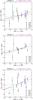 |
Fig. 9 Ionization plotted against luminosity for all Ark 564 RGS observations. The panels correspond to the three phases and the best-fit line (purple) and error in the best fit (grey), along with the Pearson coefficient r are also shown. Top: Phase 1 (ξ ≃ −0.25, gradient: 0.46 ± 0.31); Centre: Phase 2 (ξ ≃ 1.37, gradient: 1.41 ± 0.82); Bottom: Phase 3 (ξ ≃ 2.38, gradient: 0.90 ± 0.59). It seems ξ and L are linked, but in an imperfect correlation that is possibly due to sparse data for Ark 564. |
4.3. Constraints on warm absorber location
Since there are at least three independent absorbers, we can now estimate their locations, R, with respect to the source. By integrating the 2011 SED (Fig. 1), we can estimate the ionizing luminosity which, between 1 and 1000 Rydberg, gives Lion = 6.9 × 1037 W. This can be related to the absorbing source by the definition of ξ (Sect. 3.5) and following Smith et al. (2008), we assume that the thickness (Δr) of any ionised gas phase has to be less than or equal to its distance (R) from the source or  (1)and since the neutral Hydrogen column density (NH) can be related to the number density as
  (2)we can provide an expression for the upper limit of the gas cloud location as
  (3)with the NLS1 volume filling factor, Cv estimated following Blustin et al. (2005) for each phase by matching outflow momentum with scattered and absorbed radiation momentum giving
  (4)with the components defined in Appendix A and values listed in Table 4. Since Phase 3 is consistent with negligible outflow, we prefer not to average the remaining two covering factors but instead use the mean Cv = 0.03 for NLS1s, as obtained by Blustin et al. (2005). Thus we obtain upper limits for the distances from the source: Phase 1 = 74 kpc, Phase 2 = 864 pc, and Phase 3 = 37 pc.
For a more robust estimate to the absorber distances we make use of the recombination timescale, τrec. This defines how quickly the gas in the outflow is able to adjust to changes in ionisation and is related to the density nH and recombination rate αr(Xi) from ion Xi + 1 to ion Xi by ![\begin{equation} \centering \tau_{\mathrm{rec}}(X_{{i}}) = \left({\alpha_{\rm {r}}(X_{{i}})n \left[\frac{f(X_{{i+1}})}{f(X_{{i}})} - \frac{\alpha_{{\rm r}}(X_{{i-1}})}{\alpha_{{\rm r}}(X_{{i}})}\right]}\right)^{-1}\label{trec} , \end{equation}](/articles/aa/full_html/2016/02/aa27047-15/aa27047-15-eq103.png) (5)where f(Xi) is the fraction of all atoms of the element in ionisation state Xi.
(5)where f(Xi) is the fraction of all atoms of the element in ionisation state Xi.
For each absorption phase, using the spex tool “rec_time” we calculate the product nH × t for the strongest lines (in this case, Fe and O). Here, in principle, we should use ions with the highest concentrations but where τrec is negative, i.e. the ion recombines to a lower state, we use the next strongest absorption after the first positive τrec to avoid instability near turn-around in polarity. Then, assuming that the fastest recombination would occur on the shortest timescale of observations (τobs ~ 6 days), we can obtain a lower limit for nH:  (6)and then using ξ = L/nr2, we obtain revised limits (Table 4) for the cloud locations with the innermost absorber being at about 4 pc from the source. Smith et al. (2008) constrained the warm-absorbers to be between 100 pc−1000 kpc. We therefore report distance estimates improved by nearly two orders of magnitude. However, as was noted earlier, during the 2011 observations, ξ changes for all three phases (Figs. 8b−d) and the change is observed on the timescales of ~6 days (the sampling period of the 2011 observations). But since the data are sparse, it is possible the changes could be even faster; evidence of this is the correlation between ξ and L which is imperfect (Fig. 9), with the imperfections maybe pointing to faster timescales. This suggests that the gas could be responding to luminosity changes in less than six days which would imply higher nH and thus much lower distance estimates than those derived here.
4.4. Outflow kinetics
Using constraints on the location of the warm absorbers, we can now estimate the kinetics of the outflowing material. Following Crenshaw & Kraemer (2012) the mass outflow rate (Ṁout) and Kinetic Luminosity, Lkin are given by
 where we use the outflow velocity (vout) as in Table 4. Again, to provide conservative estimates, we use the typical average volume-filling factor for NLS1s of Cv = 0.03, similar to that obtained for Phase 1 in Ark 564. Ignoring Phase 3 (since it is consistent with negligible outflow), we find Ṁout ~ 0.1−2.0 M⊙ yr-1 and Lkin/Lbol ~ 0.0002%−0.01% for Phase 1 and Phase 2, respectively. We note that, in their analysis of 23 AGN, Crenshaw & Kraemer (2012) use a global covering factor of 0.5 for their estimates, which would scale our numbers by two orders of magnitude. Given that the warm absorbers in the case of Ark 564 are not co-located, we prefer to use the average covering factor for this source.
4.5. Outflow strength and impact on host galaxy
The outflow velocities for Ark 564 are lower than are generally expected of NLS1s, given the high accretion rate relative to Eddington Luminosity (Boroson 2002). A number of factors could be responsible for the weak outflows. Firstly, if the outflows are radiation pressure-driven, then the intrinsic variability of the source, and thus of the accretion rate, could naturally force material at different strengths. Secondly, orientation of the source relative to the observer could play a role, where the highest velocity components will be detected if the outflowing gas is perfectly in the line of sight. It thus follows that only the transverse component would be seen at any deviation from this angle. Ramírez (2013) also find similar weak outflows in Ark 564 and suggest that this component could belong to the base of the wind in the accretion disk comparing it to the situation with NGC 4051, which is likely to be oriented at an angle of δ ~ 30° (Krongold et al. 2007). In our analysis, if the N VII and O VIII relativistic lines are at all statistically significant (Δχ2 ~ 500 for 1490 d.o.f.), then we can thus support this argument as the laor profile predicts a disk at inclination angle of 37°± 0.5°.
Ark 564 does not seem to have extreme mass outflow rate and kinetic luminosity, with a maximum Lkin/Lbol ~ 0.01%. Our estimates are very similar to those derived using the Chandra 2008 data analysed by Gupta et al. (2013). Moreover, Blustin et al. (2005) collated high-resolution spectroscopy results for 23 AGN and found the median Macc ~ 0.04 M⊙ yr-1 and Ṁout ~ 0.3 M⊙ yr-1, which would suggest that Ark 564 has kinetics of a very typical Seyfert. For an AGN to impact the host galaxy, models require between Lkin/Lbol ~ 0.1% (Hopkins & Elvis 2010) and ~5% (Di Matteo et al. 2005). It would thus appear that, in its current state, there is no significant feedback from the AGN to its host environment in Ark 564. However, these ionized outflows are believed to be long-lived, matching the typical AGN lifetime of ~107 yr during which the warm absorbers may travel out to a few kpc and deposit up to 1054 erg s-1 even with weak outflows, such as observed for Ark 564. This is only an order of magnitude smaller than typical energies required to heat the ISM to T ~ 107 K and affect star formation (Krongold et al. 2007). Lastly, while the upper limit to the location of the Phase 1 absorber (74 kpc) does suggest it might be sustained by processes different to the ones responsible for Phase 2, the fact that both these absorbers have similar kinetics lends further support to the idea that ionized outflows could be long-lived and thus could affect the host galaxy over a typical AGN lifetime.
5. Summary
Ark 564 is a well studied source across different wavelengths and here we performed high-resolution X-ray spectroscopy on the combined data set from all XMM-Newton observations of this source. We determined the SED using a broadband continuum model for AGN and carried out photoionisation modelling on it. We detect Gaussian-broadened emission lines from three distinct zones: C, N, and O Lyα (σ ~ 900 km s-1), N VI intercombination (i) (σ ~ 500 km s-1), and O VII & Ne IX forbidden (f) (σ ~ 100 km s-1). The significant presence of (i) and (f), relative to resonance lines, also suggests photoionisation equilibrium (PIE) and so we used the XABS model to calculate transmission through a slab of material that has been ionized by the central source and detect three phases of warm absorbers with different ionisation parameters (−0.25 to 2.38). Also, we found that these gas phases are not in pressure equilibrium and are not co-located, with the highest ionized phase possibly beyond 4 pc from the source. We also report two possible broad relativistic lines, although the RGS calibration uncertainties around the same wavelengths cast doubt on their presence. Using results from the stacked spectrum, we provide best-fit parameters for the individual observations and searched for variability of luminosity and gas response to this. We find that the ionisation parameter seems to follow changes in luminosity, although not in a fully correlated way. Although the outflow velocities found here were weak, we made estimates on the kinetics of outflowing gas and find that, in its current state, the AGN in Ark 564 is unlikely to disrupt the host galaxy, although over the typical lifetimes of active galaxies enough energy can be deposited into the ISM such that star formation can be affected.
References
- Antonucci, R. 1993, ARA&A, 31, 473 [Google Scholar]
- Blustin, A. J., Page, M. J., Fuerst, S. V., Branduardi-Raymont, G., & Ashton, C. E. 2005, A&A, 431, 111 [NASA ADS] [CrossRef] [EDP Sciences] [Google Scholar]
- Boroson, T. A. 2002, ApJ, 565, 78 [NASA ADS] [CrossRef] [Google Scholar]
- Branduardi-Raymont, G., Sako, M., Kahn, S. M., et al. 2001, A&A, 365, L140 [NASA ADS] [CrossRef] [EDP Sciences] [Google Scholar]
- Calafut, V., & Wiita, P. J. 2015, JA&A, 36, 255 [NASA ADS] [Google Scholar]
- Cardelli, J. A., Clayton, G. C., & Mathis, J. S. 1989, ApJ, 345, 245 [NASA ADS] [CrossRef] [Google Scholar]
- Costantini, E., Gallo, L. C., Brandt, W. N., Fabian, A. C., & Boller, T. 2007, MNRAS, 378, 873 [NASA ADS] [CrossRef] [Google Scholar]
- Crenshaw, D. M., & Kraemer, S. B. 2012, ApJ, 753, 75 [NASA ADS] [CrossRef] [Google Scholar]
- Crenshaw, D. M., Kraemer, S. B., Turner, T. J., et al. 2002, ApJ, 566, 187 [NASA ADS] [CrossRef] [Google Scholar]
- Dewangan, G. C., Griffiths, R. E., Dasgupta, S., & Rao, A. R. 2007, ApJ, 671, 1284 [NASA ADS] [CrossRef] [Google Scholar]
- Di Matteo, T., Springel, V., & Hernquist, L. 2005, Nature, 433, 604 [NASA ADS] [CrossRef] [PubMed] [Google Scholar]
- Ebrero, J., Kriss, G. A., Kaastra, J. S., et al. 2011, A&A, 534, A40 [NASA ADS] [CrossRef] [EDP Sciences] [Google Scholar]
- Fabian, A. C., Vaughan, S., Nandra, K., et al. 2002, MNRAS, 335, L1 [NASA ADS] [CrossRef] [Google Scholar]
- Ferland, G. J., Korista, K. T., Verner, D. A., et al. 1998, PASP, 110, 761 [Google Scholar]
- Giustini, M., Turner, T. J., Reeves, J. N., et al. 2015, A&A, 577, A8 [NASA ADS] [CrossRef] [EDP Sciences] [Google Scholar]
- Gliozzi, M., Brinkmann, W., Räth, C., et al. 2002, A&A, 391, 875 [NASA ADS] [CrossRef] [EDP Sciences] [Google Scholar]
- Guilbert, P. W., McCray, R., & Fabian, A. C. 1983, ApJ, 266, 466 [NASA ADS] [CrossRef] [Google Scholar]
- Gupta, A., Mathur, S., Krongold, Y., & Nicastro, F. 2013, ApJ, 768, 141 [NASA ADS] [CrossRef] [Google Scholar]
- Hopkins, P. F., & Elvis, M. 2010, MNRAS, 401, 7 [NASA ADS] [CrossRef] [Google Scholar]
- Kaastra, J. S., Mewe, R., & Nieuwenhuijzen, H. 1996, in UV and X-ray Spectroscopy of Astrophysical and Laboratory Plasmas, eds. K. Yamashita & T. Watanabe, 411 [Google Scholar]
- Kaastra, J. S., Steenbrugge, K. C., Raassen, A. J. J., et al. 2002, A&A, 386, 427 [NASA ADS] [CrossRef] [EDP Sciences] [Google Scholar]
- Kaastra, J. S., de Vries, C. P., Steenbrugge, K. C., et al. 2011, A&A, 534, A37 [NASA ADS] [CrossRef] [EDP Sciences] [Google Scholar]
- Kalberla, P. M. W., Burton, W. B., Hartmann, D., et al. 2005, A&A, 440, 775 [NASA ADS] [CrossRef] [EDP Sciences] [Google Scholar]
- Komossa, S., & Mathur, S. 2001, A&A, 374, 914 [NASA ADS] [CrossRef] [EDP Sciences] [Google Scholar]
- Krolik, J. H., & Kriss, G. A. 2001, ApJ, 561, 684 [NASA ADS] [CrossRef] [Google Scholar]
- Krongold, Y., Nicastro, F., Elvis, M., et al. 2005, ApJ, 620, 165 [NASA ADS] [CrossRef] [Google Scholar]
- Krongold, Y., Nicastro, F., Elvis, M., et al. 2007, ApJ, 659, 1022 [NASA ADS] [CrossRef] [Google Scholar]
- Laor, A. 1991, ApJ, 376, 90 [NASA ADS] [CrossRef] [Google Scholar]
- Leipski, C., Falcke, H., Bennert, N., & Hüttemeister, S. 2006, A&A, 455, 161 [NASA ADS] [CrossRef] [EDP Sciences] [Google Scholar]
- Lodders, K., Palme, H., & Gail, H.-P. 2009, Landolt Börnstein, 44 [Google Scholar]
- Matsumoto, C., Leighly, K. M., & Marshall, H. L. 2004, ApJ, 603, 456 [NASA ADS] [CrossRef] [Google Scholar]
- Mehdipour, M., Kaastra, J. S., & Raassen, A. J. J. 2015, A&A, 579, A87 [NASA ADS] [CrossRef] [EDP Sciences] [Google Scholar]
- Mewe, R., Gronenschild, E. H. B. M., & van den Oord, G. H. J. 1985, A&AS, 62, 197 [NASA ADS] [Google Scholar]
- Nandra, K., & Pounds, K. A. 1994, MNRAS, 268, 405 [NASA ADS] [CrossRef] [Google Scholar]
- O’Donnell, J. E. 1994, ApJ, 422, 158 [NASA ADS] [CrossRef] [Google Scholar]
- Osterbrock, D. E., & Pogge, R. W. 1985, ApJ, 297, 166 [NASA ADS] [CrossRef] [Google Scholar]
- Papadakis, I. E., Brinkmann, W., Page, M. J., McHardy, I., & Uttley, P. 2007, A&A, 461, 931 [NASA ADS] [CrossRef] [EDP Sciences] [Google Scholar]
- Pinto, C., Kaastra, J. S., Costantini, E., & de Vries, C. 2013, A&A, 551, A25 [NASA ADS] [CrossRef] [EDP Sciences] [Google Scholar]
- Ramírez, J. M. 2013, A&A, 551, A95 [NASA ADS] [CrossRef] [EDP Sciences] [Google Scholar]
- Reynolds, C. S., & Fabian, A. C. 1995, MNRAS, 273, 1167 [NASA ADS] [CrossRef] [Google Scholar]
- Schlegel, D. J., Finkbeiner, D. P., & Davis, M. 1998, ApJ, 500, 525 [NASA ADS] [CrossRef] [Google Scholar]
- Shang, Z., Brotherton, M. S., Wills, B. J., et al. 2011, ApJS, 196, 2 [NASA ADS] [CrossRef] [Google Scholar]
- Silk, J., & Mamon, G. A. 2012, RA&A, 12, 917 [Google Scholar]
- Smith, R. A. N., Page, M. J., & Branduardi-Raymont, G. 2008, A&A, 490, 103 [NASA ADS] [CrossRef] [EDP Sciences] [Google Scholar]
- Steenbrugge, K. C., Kaastra, J. S., Crenshaw, D. M., et al. 2005, A&A, 434, 569 [NASA ADS] [CrossRef] [EDP Sciences] [Google Scholar]
- Steenbrugge, K. C., Kaastra, J. S., Detmers, R. G., et al. 2011, A&A, 534, A42 [NASA ADS] [CrossRef] [EDP Sciences] [Google Scholar]
- Torresi, E., Grandi, P., Costantini, E., & Palumbo, G. G. C. 2012, MNRAS, 419, 321 [NASA ADS] [CrossRef] [Google Scholar]
- Ursini, F., Boissay, R., Petrucci, P.-O., et al. 2015, A&A, 577, A38 [NASA ADS] [CrossRef] [EDP Sciences] [Google Scholar]
- Vignali, C., Brandt, W. N., Boller, T., Fabian, A. C., & Vaughan, S. 2004, MNRAS, 347, 854 [NASA ADS] [CrossRef] [Google Scholar]
Appendix A
Following Blustin et al. (2005), we assume that the momentum of the outflow matches the sum of the momentum of the absorbed and scattered radiation. The basic equations used to estimate the volume filling factor are as follows:  (A.1)with the ionising luminosity Lion = 6.9 × 1037 W for Ark 564. The AGN solid angle is taken as Ω ~ 1.6. To calculate the absorbed luminosity we applied our xabs parameters to the 2011 SED to obtain the transmission of each warm absorber. Thus,
  (A.2)where the summation is over all energy bins. This gives the expression for absorbed momentum as
  (A.3)For the scattered radiation momentum, we use the optical depth (τT = σTNH) of the absorber with column density NH and Thomson cross-section σT to obtain
  (A.4)Table 4 lists the Labs for Phases 1 and 2, which both show outflows. Note that in this scheme, Phase 3 is closest to the source and so Phase 1 is the outermost absorber. Also, since Phase 3 does not show any outflow, we cannot estimate a physical volume-filling factor for this particular absorber, unlike the other two mentioned above.
Appendix B
Table B.1 on the following page presents the best-fit parameters obtained for the individual observations as discussed in Sect. 4.2. This was achieved by freezing all best-fit parameters from the stacked spectrum, except for the flux-normalisation and ionisation parameter (ξ).
All Tables
Summary of the spectral features (other than narrow emission lines) and best-fit parameters used to model the stacked spectrum of Ark 564, resulting in a final χ2/ d.o.f. = 5178/3034.
All Figures
|
Fig. 1 Spectral energy distribution of Ark 564, derived using the EPIC-pn and OM data of 2011 XMM-Newton observations. |
| In the text | |
|
Fig. 2 Weakness of galactic neutral iron in gas form (red curve) in the line of sight to Ark 564 predicted by NH = 5.34 × 1020 cm-2 (Kalberla et al. 2005), suggesting the presence of Fe in dust form (blue curve) in our own Galaxy. |
| In the text | |
|
Fig. 3 Blow-up of the high resolution RGS spectrum of Ark 564 showing important emission and absorption lines between 7−22 Å, as discussed in the text. The best-fit final full spectrum (7−38 Å) with residuals is shown in Fig. 5. |
| In the text | |
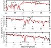 |
Fig. 4 Same as Fig. 3 but between 22−38 Å. |
| In the text | |
|
Fig. 5 Sstacked XMM-Newton RGS high-resolution spectrum produced by combining all Ark 564 RGS observations to date (in black). The final best fit (in red) consists of galactic absorption, broad and narrow Gaussian emission lines, three phases of photoionized warm-absorbers, all on a continuum modelled by spline interpolation. Lower panel: residuals (black) for this fit. |
| In the text | |
|
Fig. 6 Spline continuum with fitting for broad relativistic lines. The error bars are insignificant as is illustrated in the blow-up of the relevant region: N VII (24.73 Å) and O VIII (18.94 Å) in the laboratory frame. |
| In the text | |
|
Fig. 7 Stability curve with the positions indicated of the three warm absorbers from our best fit for Ark 564. The absence of a region with negative slope on the S-curve indicates there are no unstable regions i.e. gas can exist in equilibrium throughout the curve. This is likely due to the steep soft-excess seen in Ark 564, which allows gas to cool efficiently by lowering the Compton temperature. (Marker size exaggerated to show against small error bars in green.) |
| In the text | |
|
Fig. 8 a) Based on the best-fit parameters from the stacked spectrum we derive luminosities for all the individual observations between 2000−2011. The individual data sets are highlighted and so the combined plot is not evenly spaced in time. Observation # are as in Table 1. b), c) and d) Ionisation parameter (ξ) for the individual observations derived using stacked spectrum. Compared to a) it seems ξ varies in response to changing source luminosity. The response time is related to the gas density so the component in phase 3 is possibly denser than the remaining two warm-absorbers. |
| In the text | |
|
Fig. 9 Ionization plotted against luminosity for all Ark 564 RGS observations. The panels correspond to the three phases and the best-fit line (purple) and error in the best fit (grey), along with the Pearson coefficient r are also shown. Top: Phase 1 (ξ ≃ −0.25, gradient: 0.46 ± 0.31); Centre: Phase 2 (ξ ≃ 1.37, gradient: 1.41 ± 0.82); Bottom: Phase 3 (ξ ≃ 2.38, gradient: 0.90 ± 0.59). It seems ξ and L are linked, but in an imperfect correlation that is possibly due to sparse data for Ark 564. |
| In the text | |
Current usage metrics show cumulative count of Article Views (full-text article views including HTML views, PDF and ePub downloads, according to the available data) and Abstracts Views on Vision4Press platform.
Data correspond to usage on the plateform after 2015. The current usage metrics is available 48-96 hours after online publication and is updated daily on week days.
Initial download of the metrics may take a while.