© ESO, 2016

1. Introduction

Almost every physics text book treats the Kepler problem: the motion of two point-like masses under their mutual gravitational attraction, with the result (known already to Newton) that the orbits are closed ellipses in an orbital plane fixed in space. In practice, astrophysical bodies are not point-like, and both rotation and tidal forces lead to non-spherically symmetric and even non-axisymmetric mass distributions that do produce pure $\frac{\mathrm{1}}{\mathit{r}}$ potentials. Furthermore, perturbations by other bodies in the system as well as relativistic effects may also play a role. As a result, the actual orbits of the bodies are only approximately described by ellipses, and both the parameters of the orbit ellipse and the orbit plane itself are subject to periodic or secular changes. These effects are well known in the solar system, where the relativistic perihelion advance enjoys the greatest prominence, since this advance provides one of the best-known tests of general relativity. It is often overlooked, however, that Mercury’s relativistic perihelion advance (of 43′′ per century) constitutes only less than one percent of the overall perihelion advance observed for Mercury, which can be entirely accounted for by classical mechanics (see discussion in Misner et al. 1973).

In stellar astrophysics the analog to Mercury’s perihelion advance is known as apsidal motion, and quite a few studies of apsidal motion have been carried out in the past decades in binary systems with eccentric orbits; a catalog of such systems has been presented by Petrova & Orlov (1999, 2002) and Bulut & Demircan (2007). In this context, systems such as DI Her (Claret et al. 2010) appeared puzzling since they seemed to defy general relativity. Studying the Rossiter-McLaughlin effect, Albrecht et al. (2009) were able to demonstrate, however, that a misalignment of the orbit and spin axes in DI Her is responsible for this ostensible contradiction; more recently, an extensive review of this effect was reported as well (Albrecht 2012).

Shakura (1985) derived an expression (his Eq. (3)) for the expected apsidal motion in a binary system in an eccentric orbit that is subject to tidal forces, allowing arbitrary orientations of the rotation axes of both components and including the expected relativistic contribution to the observed apsidal motion. The expected relativistic contribution depends only on the total mass, the semi-major axis and the system eccentricity, that is, parameters that can be rather straightforwardly measured (at least for eclipsing systems). The tidal and rotational terms, in contrast, depend on the rotation rates and the orientation of the rotation axes of both components, as well as on the so-called internal structure constants (Hejlesen 1987), which describe the mass concentration inside the stars. These latter parameters are far more difficult to observe, and the structure constants can only be inferred from models. Therefore, a measurement (and correct interpretation) of apsidal motion allows observational inferences both on the interior stellar structure and on the orientation of rotation and orbit axes, which explains the great interest in apsidal motion measurements in a stellar astrophysics context.

Naturally, double-lined eccentric eclipsing systems are particularly interesting in this context: the eclipses allow a determination of the inclination angle i of the orbital plane, the line systems a determination of the projected rotational velocities and Rossiter-McLaughlin measurements of both components, and finally, apsidal motion can be addressed either through measuring the evolution of the orbit parameters or through eclipse-timing measurements, since the period between two subsequent primary and secondary eclipses differs (Rudkjøbing 1959).

One of the few binary systems for which all these measurements are possible is the system α CrB, which is – after δ Vel (cf. Pribulla et al. 2011) – the second-brightest known eclipsing system; a detailed review of the system has been given by Tomkin & Popper (1986). The α CrB system consists of an A- and G-type dwarf star in a 17.36-day orbit with substantial eccentricity (ϵ ≈ 0.37). Since the system is viewed almost edge-on (i = 88.2°), both the primary eclipses, when the secondary G-type star appears in front of the brighter A-type primary, and secondary eclipses with the opposite viewing configuration can be observed. Light-curve modeling yields radii of 3.04 and 0.92 R_⊙, respectively, for the primary and secondary components (Tomkin & Popper 1986), which means that the primary eclipse is only partial, while the G-type component is entirely occulted by the primary component during the secondary eclipse.

α CrB is also a spectroscopic binary with lines from both components visible in the spectrum. Therefore a full solution of the binary orbit is possible, as is a determination of individual stellar masses and radii. Tomkin & Popper (1986) derived accurate system parameters for both components from their own observations of the secondary component (taken in the years 1979–1984) and from the primary component (taken in the years 1959–1961 by Ebbighausen 1976 and from the photometry of Kron & Gordon 1953) and concluded that the primary component, that is, α CrB A, is a slightly evolved star of spectral type A0, while the secondary is a G5 star essentially on the zero-age main sequence and therefore young, at least when compared to the Sun. This finding is in line with the X-ray emission observed from the α CrB system, first detected by Schmitt & Kürster (1993), who demonstrated the total nature of secondary minimum, when the system’s X-ray flux is totally eclipsed. This means that the whole X-ray emission from the system is produced by the late-type companion, in line with the standard rotation-age-activity paradigm (Schmitt & Kürster 1993).

Finally, the α CrB system is very interesting from its evolutionary point of view: the secondary’s rotation velocity of ≈15 km s^-1, as reported by Tomkin & Popper (1986), corresponds to a rotation period of about five days, and the primary’s rotational velocity of 138 km s^-1 (Royer et al. 2002) corresponds to a period shorter than one day, which means that both rotation periods are much shorter than the orbit period of 17.3599 days. The system is therefore neither synchronized nor circularized, which makes the question of the alignment of the rotation axes of the two components with the orbit axis particularly interesting.

The very rapid rotation of the primary in the α CrB system is expected because it does not possess any convective envelope, which is required for the dissipation of angular momentum in interaction with tidal bulges (see Zahn 1989). By contrast, the G-star primary with its convective envelope has already slowed down noticeably, although it still rotates much faster than the Sun. The rapid primary rotation gives rise to substantial quadrupole moments in the external gravitational field and thus to apsidal motion, given the system’s eccentricity. Volkov (1993, 2005) discussed timing measurements of the eclipses of α CrB, Schmitt (1998) presented and discussed X-ray eclipse measurements of the secondary eclipse of α CrB, and Volkov (2005) argued that all the available eclipse measurements suggest apsidal motion at a level much lower than theoretically expected. Thus it seems appropriate to address the question of apsidal motion in the α CrB system from the point of view of radial velocities (RV), since with our new TIGRE data taken in 2014, radial velocity data spanning more than 100 years (!) are now available for the primary, and radial velocity data spanning more than 50 years for the secondary to study any secular evolution of the system. We emphasize that the method presented in this paper is applicable to any eccentric binary system with sufficient temporal data coverage, which also means non-eclipsing systems; we will address the question of the periods between primary and secondary minima in a separate paper (cf. Schmitt, in prep.).

The plan of our paper is as follows: in Sect. 2 we present new radial velocity data of the two components of α CrB taken in 2014 with our TIGRE facility, in Sect. 3 we address the question of apsidal motion in the α CrB system and summarize our approach to modeling the radial velocities curves observed over the past 100 years. In Sect. 4 we present our conclusions. A few formulae that we used in our analysis and that are scattered over the literature are summarized in an appendix.

2. Observations and data analysis

The new observations we present here have been carried out with the TIGRE facility, a new robotic spectroscopy telescope located in central Mexico at the La Luz Observatory of the University of Guanajuato. The TIGRE 1.2 m telescope is fiber-coupled to an échelle spectrograph with a spectral resolving power exceeding 20 000 over most of the covered spectral range between 3800 Å and 8800 Å, with a small gap of about 130 Å around 5800 Å. The distinct feature of TIGRE is its robotic operation, that is, it (normally) carries out all observations without any human intervention. A robotic system such as TIGRE does require a fully automatic data reduction pipeline including an automated wavelength calibration, which is implemented in the interactive data language (IDL) environment and uses the powerful and flexible reduction package REDUCE (Piskunov & Valenti 2002), with special adaptations to the TIGRE context; a detailed description of TIGRE is given by Schmitt et al. (2014). For observations of a binary system with an orbital period of more than 17 days a robotic facility is clearly ideal. We observed the α CrB system for more than 50 nights between December 2013 and June 2014; the dates of our α CrB observations are listed in Table B.1.

2.1. Lines of the secondary component

The TIGRE spectrum of α CrB is dominated by the primary component, but in some specific spectral ranges, lines of the secondary can be clearly recognized. One such case is plotted in Fig. 1, where we show the coadded TIGRE spectrum of α CrB in the wavelength range between 6090 Å and 6140 Å, with all spectra superimposed using the wavelength shifts derived from our RV-solution for the secondary component, which lead to a corresponding smearing of all primary spectral lines (see discussion in Sect. 2.3). A corresponding (higher resolution) solar spectrum taken from Delbouille et al. (1990) and Delbouille & Roland (1995) is shown in Fig. 2. A comparison to Fig. 1 shows that all the stronger lines appearing in the solar spectrum do have their counterpart in the coadded TIGRE α CrB spectrum. This specifically applies to the “triplet” of lines between 6102 Å and 6104 Å, which arise from Fe I and Ca I with a total equivalent width of 308 mÅ (in the Sun), the Ca I line at 6122 Å with an equivalent width of 222 mÅ and the line complex that is due to Fe I between 6138 Å and 4140 Å with a total equivalent width of 330 mÅ. Many weaker lines are also visible, however.

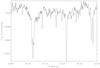Fig. 1 Coadded TIGRE spectrum of α CrB in the spectral region 6090–6140 Å. The sharp lines are all due to the secondary component; cf., Fig. 2 and discussion in text.

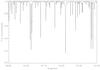Fig. 2 High-resolution solar spectrum in the spectral region 6090–6140 Å taken from Delbouille et al. (1990) and Delbouille & Roland (1995); see text for discussion.

Figure 1 is somewhat deceptive since it represents the results of more than 40 coadded spectra with individual exposure times of typically 1200 s each, but to determine the wavelength shift of each individual spectrum, only shorter integrations are available, and hence only the strong lines can and should be used for analysis. We therefore identified a few spectral ranges with strong lines attributable to the secondary. These spectral ranges comprise in particular a 5 Å wide region around 6103 Å containing the Fe I lines at 6102.18 Å and 6103.19 Å as well as the Ca I line at 6102.73 Å, a 3 Å wide region around 6122 Å containing the Ca I line at 6122.22 Å, a 3 Å wide region around 6191 Å containing an Fe I and a Ni I line, a 3 Å wide region around 6400 Å containing Fe I lines, a 3 Å wide region around 6421.4 Å containing again Fe I and Ni I lines, and a 3 Å wide region around 6439 Å with Fe I lines.

2.2. Radial velocity curve: primary

To determine the radial velocity of the primary component we considered the spectral region between 6330 Å and 6380 Å, where two Si II lines are located at 6347.11 Å and 6371.37 Å. This spectral range lies very close to the O₂ absorption band starting at 6275 Å, and numerous telluric lines are present in this spectral region. We constructed a sample telluric absorption spectrum using the ESO molecfit package (Kausch et al. 2014) and examined the positions of the strongest lines in the spectral region considered. The Si II lines were modeled as rotationally broadened absorption lines with v sin(i) = 138 km s^-1 (Royer et al. 2002) and an instrumental Gaussian broadening corresponding to a resolution of 20 100. The Si II lines were allowed to have variable wavelength positions but had fixed wavelength differences, while the stronger telluric absorption lines were modeled as instrumentally broadened lines with fixed wavelengths but individually variable amplitudes; the remaining continuum variations were described by a sum of low-order (Legendre) polynomials. We determined the best fit through a χ²-statistics by varying the centroid position of the Si II lines (but keeping their wavelength separation fixed). As an example of this procedure, we show in Fig. 3 one of our α CrB spectra, which shows the two Si II lines and quite a few telluric absorption lines; clearly, the telluric absorption lines provide a wavelength grid against which the position of the Si II lines can be well determined. The resulting radial velocity data are provided in Table B.1 and are graphically shown in Fig. 4 together with a model curve; the O–C values are shown in the lower panel.

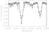Fig. 3 TIGRE spectrum of α CrB in the spectral range 6330–6380 Å together with model fit; the sharp lines are telluric, the two broad lines are produced by Si II; see text for details.

Fig. 4 Upper panel: TIGRE RV curve for the primary (asterisk) and secondary (diamonds) of the α CrB system with model curves derived from Eq. (A.1) with model parameters listed in Table 1. Lower panel: O–C points for the primary (asterisk) and secondary (diamonds).

2.3. Radial velocity curve: secondary

To determine the projected radial velocity of the secondary component in each of our measured spectra, we used a template high-resolution solar spectrum using the solar atlas by Delbouille et al. (1990) and Delbouille & Roland (1995), extracted the appropriate regions in our α CrB spectra (cf. Sect. 2.1), and proceeded to calculate the cross correlation function between these spectra. We identified the maximum of the measured cross correlation function as the wavelength and hence velocity shift between the two spectra. Since the individual spectra of α CrB are much noisier than the summed spectra shown in Fig. 1 and the secondary lines are seen as rather weak lines on the continuum of the A-type primary, the peaks of the cross correlation are well below unity and some cross correlation functions show multiple or not clearly defined peaks. We therefore rejected all spectra where the cross correlation function did not exceed 0.4 and did not show a clearly defined single maximum. The resulting RV data are also provided in Table B.1, and in Fig. 4 we show the resulting radial velocity curve together with a model curve; the O–C values are shown in the lower panel.

2.4. System parameters from the RV curve

With our new RV data presented in Table B.1 we can determine new system parameters using the RV curve in Eq. (A.1). Since in contrast to Tomkin & Popper (1986) the RV data for both components were taken at the same epoch, we carried out a simultaneous fit of both components using the same eccentricity, the same time of periapsis passage, and arguments of periapsis differing by exactly 180 degrees for the two components, while we of course allowed for different K values and different velocity offsets for the two components to absorb errors in the wavelength scale. We set up a Markov chain Monte Carlo (MCMC) scheme, and after an initial burn-in considered chain lengths of 300 000 iterations with acceptance rates typically on the order of 60%, from which we determined the mean and variance of each parameter. We list them in Table 1 for the fits of the A component, B component and the joint fit. For the joint fit we also list the resulting mass ratios, the semi-major axis (multiplied by sin(i)) and total mass (multiplied by sin³(i)) together with their errors. It is reassuring that the parameters derived for the A and B components separately and those derived from the joint fit are consistent with each other. Our TIGRE data are new in the sense that for the first time, they allow determining the argument of the periapsis derived for both components with simultaneously taken data.

We examined our MCMC results for correlations between the fit parameters and found a very obvious correlation between the derived times of periapsis passage and arguments of periapsis, which can be readily attributed to the second term in Eq. (2): a higher value of the argument of the periapsis can be compensated for by a lower value of the true anomaly, which is achieved with an earlier periapsis passage. In Fig. 5 we show the results of our MCMC result for the argument of the periapsis and the derived time of periapsis passage together with the 50%, 90%, and 99% error ellipses.

To be able to compare our results to the literature values, we also carried out the same exercise for the RV data presented by Tomkin & Popper (1986), the only difference being the treatment of the times of periapsis passage, which were fitted separately since these data were taken more than 30 years apart for the A and B components (see Tomkin & Popper 1986, for details). To facilitate the comparison, the results of this analysis are listed in Table 2.

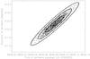Fig. 5 MCMC chain parameters (argument of periapsis and time of periapsis passage; note that only every 100th point is plotted) for the TIGRE data, showing the correlation between these parameters. The solid contours contain 50%, 90%, and 99% of the data points.

Our results are largely consistent with the literature results presented by Tomkin & Popper (1986). In general, our errors are smaller and we favor a slightly higher value for the system eccentricity. In addition, our values for the total mass are somewhat lower, and we favor a slightly more massive secondary component. Unfortunately, the results for the argument of the periapsis cannot be readily compared. The error for the argument of periapsis is very large when only the A component is considered. When only the B component or both components are considered, our new values are higher, but not significantly so, thus no conclusions on apsidal motion can be drawn from these data (yet).

2.5. Rotational velocity: secondary

To our knowledge, no precise determinations of the rotation velocity v sin (i) of the secondary have been published; Tomkin & Popper (1986) quoted a value of v sin (i) ~ 15 km s^-1 without providing any further evidence for this value. To address the question of the secondary’s rotation we specifically considered the spectral range between 6000–6105 Å, where two strong Fe II and Ca I lines are located in the solar spectrum (cf. Fig. 6). Convolving this solar spectrum with various v sin (i) values and the TIGRE instrumental resolution suggests rotation velocities between 5–10 km s^-1 (cf. Fig. 7), and we conclude that a more reliable determination of the secondary’s rotational velocity requires spectra with higher spectral resolution than TIGRE can provide. At any rate, a rotational velocity of 5–10 km s^-1 corresponds to rotation periods of about 7–14 days (assuming aligned orbit and secondary spin axes), which is consistent with the observed X-ray activity of α CrB B (Schmitt & Kürster 1993).

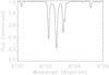Fig. 6 Excerpt of high-resolution solar spectrum in the spectral range 6100–6106 Å taken from Delbouille et al. (1990) and Delbouille & Roland (1995); see text for details.

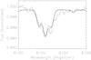Fig. 7 Coadded TIGRE spectra (solid histogram) together with the solar spectrum (shown in Fig. 6) convolved with the TIGRE spectral resolution and v sin (i) values of 5 km s-1 (solid line), 10 km s-1 (long dashed line), and 15 km s-1 (short dashed line).

3. Apsidal motion in α CrB

3.1. Expected effects in the α CrB system

Applying the apsidal motion formula given by Shakura (1985), we can compute the expected values for the α CrB system as a function of the misalignment angle between the rotation axis of the primary and the orbit axis; for simplicity, we assume that the rotation axes of primary and secondary are parallel, but we note that – naturally – the primary accounts for by far the largest contribution. As stellar structure constants we used the same values as Schmitt (1998), that is, k₂ = 0.0049 (note the typo in Table 3 in Schmitt 1998) for the primary and k₂ = 0.021 for the secondary. The resulting curve of apsidal motion rate vs. misalignment angle is shown in Fig. 8, which demonstrates that the rotational contribution indeed dominates over the expected tidal and relativistic contributions, and that a severe misalignment between the rotation and orbit axes could indeed lead to apsidal motion values in apparent contradiction of general relativity and even to retrograde apsidal motion.

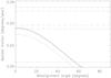Fig. 8 Expected apsidal motion in the α CrB system; total effect (solid line), rotational contribution (dashed line), relativistic contribution (dash-dotted line), and tidal contribution (dotted). The dash-dotted lines denote the 68% and 90% uncertainty ranges for the derived apsidal motion; see text for details.

3.2. Application to observations

All this very clearly shows that some apsidal motion is expected to occur in the α CrB system. According to the theory sketched in Appendix A.2, we expect a linear secular change of the argument of the periapsis through $\mathit{\omega }\mathrm{\left(}\mathit{t}\mathrm{\right)}\mathrm{=}\mathit{\omega ̇}\mathrm{(}\mathit{t}\mathrm{-}{\mathit{t}}_{\mathrm{0}}\mathrm{)}\mathrm{+}{\mathit{\omega }}_{\mathrm{0}}\mathit{,}$(1)with denoting the desired apsidal motion rate and ω₀ the argument of the periapsis at some reference time t₀. In this case there are no closed orbits, and we need to define what is meant by “period”. In particular, we need to distinguish between the anomalistic period P_A, that is, the time between two periapsis passages, the average time that is required for a full revolution of 2π and P_p and P_s, and the time span between two subsequent primary and secondary minima (cf. the discussion in Appendix A.2). It is interesting to consider the difference between the anomalistic period and the currently observed period P_p between two primary minima. Evaluating Eq. (A.24) with the nominal system parameters and assuming an apsidal motion rate of 0.035 degrees/year, we find a difference of 10.8 s. Since α CrB executes a little more than 21 revolutions in one year, the system executed more than 2100 revolutions during the more than 100 years of observations available to date. Thus the cumulative difference between these two periods is expected to be on the order of 20 000 s, or more than six hours ! At the same time, the argument of the periapsis moved by less than 4 degrees, which is difficult to detect given the quality especially of the old data (cf. Sect. 3.2). At any rate, the values of the argument of the periapsis ω and the time of periapsis passage at the present epoch cannot be independently chosen, they are instead linked by the actual value of . For the following, we therefore consider the values P_p at the current epoch and the eccentricity ϵ as known, and together with the argument of the periapsis from Eq. (1), the anomalistic period and in particular the times of periapsis passages are known. In the following we carry out two approaches to determine the apsidal motion from RV data.

3.2.1. RV fitting

Our data consist of Q different samples, taken at different epochs, each of which contains N_q observations, and we use the indices (q,j) to refer to the data that consist of the observed radial velocities rv_obs,q,j and their errors σ_q,j taken at times t_q,j. We specify our RV-model with the secular constants ϵ, the orbit eccentricity, and , the apsidal motion rate; further model parameters are the period P_p, that is, the time between primary minima, the time of periapsis passage T₀, and the argument of the periapsis at that time ω₀. With these model parameters the mean anomaly m_q,j and true anomaly θ_q,j as well as the actual argument of the periapsis ω_q,j can be computed at all observed times t_q,j, and therefore the model RVs can be expressed as $\mathit{r}{\mathit{v}}_{\mathrm{mod}\mathit{,q,j}}\mathrm{=}{\mathit{V}}_{\mathrm{0}\mathit{,q}}\mathrm{+}\mathit{K}\mathrm{\times }\mathrm{\left(}\cos \mathrm{\right(}{\mathit{\theta }}_{\mathit{q,j}}\mathrm{+}{\mathit{\omega }}_{\mathit{q,j}}\mathrm{)}\mathrm{+}\mathit{ϵ}\cos \mathrm{(}{\mathit{\omega }}_{\mathit{q,j}}\mathrm{\left)}\mathrm{\right)}\mathit{.}$(2)In Eq. (2) we treat the velocities V_0,q, q = 1...Q, as systemic velocities, or in other words, as free parameters, which allow us to absorb errors in the radial velocity scale of different data sets, while the velocity amplitude K is a free model parameter that must be the same for all observations. The model parameters are determined by minimization of the χ²-statistics given by ${\mathit{\chi }}^{\mathrm{2}}\mathrm{=}\sum _{\mathit{q}\mathrm{=}\mathrm{1}}^{\mathit{Q}}\sum _{\mathit{j}\mathrm{=}\mathrm{1}}^{{\mathit{N}}_{\mathit{q}}}\frac{\mathrm{(}{\mathit{V}}_{\mathrm{0}\mathit{,q}}\mathrm{+}\mathit{K}\mathrm{\times }{\mathit{\beta }}_{\mathit{q,j}}\mathrm{-}\mathit{r}{\mathit{v}}_{\mathrm{obs}\mathit{,q,j}}{\mathrm{)}}^{\mathrm{2}}}{{\mathit{\sigma }}_{\mathit{q,j}}^{\mathrm{2}}}\mathit{,}$(3)where ${\mathit{\beta }}_{\mathit{q,j}}\mathrm{=}\cos \mathrm{(}{\mathit{\theta }}_{\mathit{q,j}}\mathrm{+}{\mathit{\omega }}_{\mathit{q,j}}\mathrm{)}\mathrm{+}\mathit{ϵ}\cos \mathrm{\left(}{\mathit{\omega }}_{\mathit{q,j}}\mathrm{\right)}\mathit{.}$(4)Clearly, the model is linear in the parameters K and V_0,q, q = 1,Q, and minimization can be obtained through matrix inversion. Since we consider ϵ and P_p as known, only the three parameters t₀, ω₀, and remain.

3.2.2. Periapsis passage times

The RV data are often available not in a continuous fashion but only at individual epochs. For these epochs the system parameters can be obtained by fitting the data to the RV Eq. (A.1). Given L measurements of periapsis passage T_peri,l, l = 1...L and their respective errors σ_T,l, l = 1...L, we can determine the anomalistic period P_A through a minimization of the expression ${\mathit{\chi }}^{\mathrm{2}}\mathrm{=}\sum _{\mathit{l}\mathrm{=}\mathrm{1}}^{\mathit{L}}\frac{\mathrm{(}{\mathit{T}}_{\mathrm{peri}\mathit{,l}}\mathrm{-}{\mathit{P}}_{\mathrm{A}}\mathrm{\times }{\mathit{N}}_{\mathit{l}}\mathrm{-}{\mathit{t}}_{\mathrm{0}}{\mathrm{)}}^{\mathrm{2}}}{{\mathit{\sigma }}_{\mathit{T,l}}^{\mathrm{2}}}\mathit{,}$(5)where N_l denotes the number of revolutions at periapsis passage T_peri,l since some reference time t₀. If next, for example, the time span between primary minima is known (as is the case for α CrB), the period difference P_A − P_p can be calculated, and P_A − P_p also carries the desired information on apsidal motion through Eq. (A.24).

3.3. Application to α CrB

We now proceed to apply the formalism of Sect. 3.2 to the available RV data for α CrB. Clearly, any apsidal motion must be identical for both components. We specifically used our new TIGRE data (epoch 2014) and the RV data presented by Tomkin & Popper (1986) (taken at epoch 1979–1984) for the secondary component, and, for the primary component, again our new TIGRE data (epoch 2014), those by Ebbighausen (1976) (taken at epoch 1959–1961), those by McLaughlin (1934) (taken at epoch 1929–1934) and finally those by Cannon (1909) and Jordan (1910) (taken at epoch 1907–1908); it is obviously rare to find systems with RV data available covering more than one hundred years.

3.3.1. RV fitting

We now considered all available data sets simultaneously and allow . We assessed the goodness of fit with a χ²-criterion using as error estimates the observed O–C distribution. We further assumed that each data point carries the same weight, but we also experimented with different weighing schemes and are convinced that the final fit results do not depend sensitively on the weights used. The best-fit value for is 0.044 degrees/year. For this fit we left the argument of the periapsis fixed at the present epoch, but we again verified that the fit results do not depend sensitively on the precise value of ω₀. The resulting distribution of the fit quality χ² vs. is shown in Fig. 9.

Fig. 9 χ2 as a function of for the available RV data of the α CrB system; see text for details. The data clearly demand a non-zero value of .

To better assess the errors on this value, we generated 30 000 bootstrap samples of the actual observations from the derived error distribution and refitted the bootstrapped data for the value of . The resulting probability histogram on is shown in Fig. 10 together with the 68% and 90% errors; our formal best fits are $\mathit{\omega ̇}\mathrm{=}\mathrm{0.044}{\mathrm{5}}_{-0.0064}^{\mathrm{+}\mathrm{0.0063}}$ degrees/year (68% error interval) and $\mathit{\omega ̇}\mathrm{=}\mathrm{0.044}{\mathrm{5}}_{-0.0098}^{\mathrm{+}\mathrm{0.0097}}$ degrees/year (90% error interval). We also plot these values in Fig. 8 in comparison with the expected effects. As is clear from Fig. 8, the measurements lie outside the 68% but inside the 90% error intervals, slightly on the high side, but we note that the expected apsidal motion rate depends on the fifth power of the radius and measurement errors were not considered in the computation of the expected apsidal motion rate. Therefore we conclude that expectations and observations are consistent with each other, and we finally note that – as expected – the value zero, that is, no apsidal motion, is certainly excluded by the available measurements.

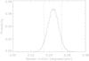Fig. 10 Probability distribution histogram for the derived bootstrapped apsidal motion rate (in degrees per year); for orientation the expected level of apsidal motion for the case of complete aligned orbit and rotation axes is also shown (cf. Fig. 8).

3.3.2. Periapsis passage times

We now examine the available data sets individually since each of them covers only a limited amount of time where the effects of apsidal motion should be very small indeed. In these fits we therefore assumed , set the eccentricity and K values to the best-fit TIGRE values and fit for the values of ω and T_peri; the results are listed in Table 3. An inspection of the relevant literature shows good agreement between the published values and our redetermined values. To estimate the errors, we generated 200 000 bootstrapped observations and carried out the corresponding fits.

We then proceeded to fit the derived periapsis passage times using Eq. (5), derived an estimate for P_A and computed P_A − P_p, using the value P_p = 17.359907 days (cf. Tomkin & Popper 1986). Again, to assess the robustness of the thus derived period difference, we bootstrapped new measurements using the estimated errors of the periapsis passage times quoted in Table 3 and thus produced the probability histogram shown in Fig. 11. To assess the influence of the old data taken before 1920, we considered all data (solid histogram) and only the data taken after 1920 (dash-dotted histogram). Considering all data, we find a mean value of ${\mathit{P}}_{\mathrm{A}}\mathrm{-}{\mathit{P}}_{\mathrm{p}}\mathrm{=}\mathrm{8.3}{\mathrm{5}}_{-2.43}^{\mathrm{+}\mathrm{2.44}}$ s (68% error interval) and ${\mathit{P}}_{\mathrm{A}}\mathrm{-}{\mathit{P}}_{\mathrm{p}}\mathrm{=}\mathrm{8.3}{\mathrm{5}}_{-4.01}^{\mathrm{+}\mathrm{4.02}}$ s (90% error interval), while excluding the data taken before 1920 leads to ${\mathit{P}}_{\mathrm{A}}\mathrm{-}{\mathit{P}}_{\mathrm{p}}\mathrm{=}\mathrm{5.4}{\mathrm{3}}_{-2.85}^{\mathrm{+}\mathrm{2.85}}$ s (68% error interval) and ${\mathit{P}}_{\mathrm{A}}\mathrm{-}{\mathit{P}}_{\mathrm{p}}\mathrm{=}\mathrm{5.4}{\mathrm{3}}_{-4.71}^{\mathrm{+}\mathrm{4.72}}$ s (90% error interval). Thus, the anomalistic period and the period between primary minima very clearly differ in the α CrB system.

Fig. 11 Bootstrapped distribution (200 000 realizations) of the derived period differences PA − Pp for the derived periapsis passage times listed in Table 3. To better illustrate the influence of the older data, a histogram with all data (solid line) and a histogram excluding the data taken before 1920 (dash-dotted line) was produced; see text for details.

4. Discussion and conclusions

As demonstrated by Figs. 9–11, apsidal motion is definitely present in the α CrB system. The available measurements, taken over the last 100 years, are consistent with theoretical expectations and, in particular, with a rotation axis of the primary more or less orthogonal to the orbit plane. Such an alignment between orbit and rotation axes in the α CrB system is also suggested by measurements of the Rossiter-McLaughlin effect for the binary component (S. Albrecht, in prep.).

Because of Eq. (A.19), these values imply a difference between orbital and anomalistic period of ΔP ≈ 5.9 s. With a time lapse of 100 years or 2104 binary revolutions, this means a difference of about 3° for the argument of the periapsis and an advance of the time of periapsis passage of about 12 410 s or 0.144 days. For our TIGRE data the accuracy of the determinations of the periapsis values is about 0.02–0.05 days, and this accuracy could be improved by further observations in the next years. For the older data, the timing accuracy is – naturally – far worse.

With the derived values of the apsidal motion rate of degrees/year the apsidal motion period P_aps must be in the range 6600 yr <P_aps< 10 600 yr, implying that the presently available observations, taken over the past 100 years, cover only a tiny fraction of the full apsidal motion cycle, and therefore the changes in the other system parameters such as the argument of the periapsis or the time between primary minima ought to be very small indeed. Furthermore, converting these values into the difference ΔP between the anomalistic period and the actual period of primary minima, we find a range 10.5 s < ΔP< 16.5 s, which is marginally consistent with the value of P_A − P_p measured for the whole data set, but is true to a lesser extent for the data excluding the data taken before 1920. While all the error intervals do not formally overlap, they are still close and indicate at least some degree of self-consistency; clearly, more accurate measurements are in order.

As discussed in detail by Rudkjøbing (1959), apsidal motion also leads to a different period between subsequent primary and secondary minima. Applying Eq. (A.28) with the α CrB system parameters and our derived apsidal motion values results in a difference 7.2 s < ΔP_sp = P_s − P_p< 11.6 s, while Schmitt (1998) derived a value of ΔP_sp = 4.8 ± 2.1 s, again outside the formal 90% interval. It is difficult to assess the precise reasons for this discrepancy, and further X-ray and optical observations would certainly help to resolve this subject matter; for the mean period P_2π this difference is in the range 6.7 s < ΔP< 10.7 s.

Our apsidal motion measurements suggest a small misalignment angle at best, and therefore the true equatorial rotation velocity v_eq of α CrB A should be close to the observed v sin (i)-value of 138 km s^-1, which allows us to compute the constant ζ through Eq. (A.43) and the structure constant log (k₂) from Eq. (A.42), where we find a best value of − 2.42 and the range − 2.35 < − log  (k₂) < − 2.55. Here we recall that Eq. (A.42) only holds in the absence of all tidal effects. Inspecting the different terms in the apsidal moment rate equation presented by Shakura (1985) (his Eq. (3)), we find that the contributions of the secondary are indeed very small (since the apsidal motion effects scale with the fifth power of radius), while the tidal effects, that is, the tides produced by the secondary on the shape of the primary, account for about 3% and the GR effect for about 7% of the overall observed apsidal motion effect. Using then Eq. (3) in Shakura (1985), we determine for the nominal case degrees/year relativistic, tidal, and rotational contributions of 10%, 3%, and 87%, respectively, with log (k₂) = −2.20. For the lower and upper bounds of 0.034 and 0.054 degrees/year we obtain relative contributions of 14%, 3%, 83% and log (k₂) = −2.33 and 9%, 3%, 88% and log (k₂) = −2.11, respectively, always assuming parallel rotation and orbital axes. Claret & Gimenez (1991) quoted for a 2.51 M_⊙ model log k₂ = −2.27 at zero age and log k₂ = −2.42 at an age of 300 Myr; these values fit our measurements reasonably well. Using the system data for α CrB as listed by Tomkin & Popper (1986) and derived in this paper, that is, ϵ = 0.379, R = 3.04 ± 0.3R_⊙, and P = 17.3599 days and the estimated stellar structure constants log (k₂), we can estimate the gravitational moment J₂ to lie in the range 0.0001 <J₂< 0.0002. This means that despite α CrB A’s rapid rotation, its J₂-value is much lower than that of the also rapidly rotating giant planet Jupiter (J_2,Jupiter = 0.015) by almost two orders of magnitude.

In summary, our apsidal motion data therefore suggest a rather close alignment between orbit axis and the rotation axis of the primary. The α CrB system is believed to be a member of the Ursa Major moving group (a detailed discussion of this moving group can be found in Soderblom & Mayor 1993). While traditionally this group was believed to have an age of 300–400 Myr, more recent studies suggest an age close to that of the Hyades (King et al. 2003), that is, around 600 Myr, in which case the models of Claret & Gimenez (1991) yield a value of log k₂ = −2.67, which is somewhat smaller than observed. On the other hand, if we use the observed radius and mass of the A1 primary star and compare it with evolution tracks with a well-tested amount of extended mixing (see Pols et al. 1997; and Schröder et al. 1997 for details), we find an age of around 400 Myr, which is about two-thirds through the primary’s main-sequence evolution. Our models would further indicate a slightly smaller radius (of 0.8 R_⊙) than the one derived by Tomkin & Popper (1986), but this discrepancy may still lie within the observational uncertainties. At any rate, either estimate makes the G-star secondary indeed very young compared to the Sun, nearly a zero-age main-sequence star.

Zahn & Bouchet (1989) argued that for stars of the Hyades age the limiting circularization period, that is, the longest period for which circular orbits are observed, is between 8.5 and 11.9 days. Thus, the α CrB system, which is younger than or approximately coeval with the Hyades, is not circularized and synchronized, which follows from its period of 17.36 days. Consequently, the observed alignment of orbit and rotation axes suggests that the system was formed in this way, and it would be very interesting to investigate the Rossiter-McLaughlin effect in the secondary of the α CrB system. This view of the formation history of the α CrB system is also supported by Herschel observations of the circumbinary disk around the α CrB binary system by Kennedy et al. (2012), who argued that the observed coplanarity of this disk with the binary orbit plane is of primordial origin.

Acknowledgments

We thank the anonymous referee of this paper for thoughtful and constructive comments that greatly helped this paper. We acknowledge the continued support by various partners who helped to realize TIGRE. In the first place, this is the University of Hamburg, which gave support in terms of funding, manpower, and workshop resources. Furthermore, grants from the Deutsche Forschungsgemeinschaft (DFG) in various funding lines is gratefully acknowledged, as well as travel money from both the DFG and DAAD, and from CONACyT in several bilateral grants, and finally CONACyT support by its mobility grant No. 207662. The Liège contribution to TIGRE is funded through an opportunity grant from the University of Liège. The Universities of Guanajuato and Liége and the Mexican state of Guanajuato shared the funding of the infrastructure required by TIGRE at the La Luz site, and there is continued support by the University of Guanajuato in terms of manpower and running costs of the facilities.

References

Appendix A: Modeling apsidal motion

Traditionally, the problem of apsidal motion determination has been approached from eclipse timing. Here we consider only radial velocity measurements, we therefore provide a somewhat more extensive collection of the relevant formulae and physical background for our approach; none of this material is really new, however, it is scattered all over the literature, and we aim at providing a compact compilation for easy reference.

Appendix A.1: Keplerian orbits

For reference, we provide the essential textbook formulae for our RV modeling as provided, for example, by Haswell (2010). The radial velocity V_r of a body in an elliptic orbit around a spherically symmetric central object is given by the expression ${\mathit{V}}_{\mathit{r}}\mathrm{=}{\mathit{V}}_{\mathrm{0}}\mathrm{+}\mathit{K}\mathrm{\left(}\cos \mathrm{\right(}\mathit{\theta }\mathrm{+}\mathit{\omega }\mathrm{)}\mathrm{+}\mathit{ϵ}\cos \mathit{\omega }\mathrm{)}\mathit{,}$(A.1)where K denotes the so-called velocity amplitude, θ the true anomaly, ω the argument of the periapsis, and ϵ the eccentricity as usual; V₀ denotes a velocity of the system’s center of mass w.r.t. the observer. The true anomaly θ is related to the eccentric anomaly E through $\tan \frac{\mathit{E}}{\mathrm{2}}\mathrm{=}{\left(\frac{\mathrm{1}\mathrm{-}\mathit{ϵ}}{\mathrm{1}\mathrm{+}\mathit{ϵ}}\right)}^{\frac{\mathrm{1}}{\mathrm{2}}}\tan \left(\frac{\mathit{\theta }}{\mathrm{2}}\right)\mathit{,}$(A.2)and the eccentric anomaly is related to the mean anomaly M through Kepler’s equation via $\mathit{E}\mathrm{-}\mathit{ϵ}\sin \mathrm{\left(}\mathit{E}\mathrm{\right)}\mathrm{=}\mathit{M}\mathit{.}$(A.3)M is a measure of time t. If T_Peri denotes the time of a given periapsis passage and the mean period of one revolution, that is, the average time of the body to cover the angular distance of 2 π, $\mathit{M}\mathrm{\left(}\mathit{t}\mathrm{\right)}\mathrm{=}\frac{\mathrm{2}\mathit{\pi }}{\mathit{P̂}\mathrm{2}\mathit{\pi }}\mathrm{·}\mathrm{(}\mathit{t}\mathrm{-}{\mathit{T}}_{\mathrm{Peri}}\mathrm{)}\mathit{,}$(A.4)which means that M(t) denotes the angle since the reference periapsis passage. The velocity amplitude K_p of the primary can be measured and is related to the other orbital elements through ${\mathit{K}}_{\mathrm{p}}\mathrm{=}\frac{{\mathit{M}}_{\sec }}{{\mathit{M}}_{\mathrm{tot}}}\frac{\mathrm{2}\mathit{\pi a}\sin \mathrm{\left(}\mathit{i}\mathrm{\right)}}{\mathit{P̂}\mathrm{2}\mathit{\pi }\sqrt{\mathrm{1}\mathrm{-}{\mathit{e}}^{\mathrm{2}}}}\mathit{,}$(A.5)where a and i denote semi-major axis and inclination and M_sec and M_tot secondary and total mass as usual; obviously, a similar formula applies to the velocity amplitude K_s of the secondary.

Appendix A.2: Apsidal motion in the gravitional field of a rotating body

The following material can be found in most textbooks on celestial mechanics, for example, Fitzpatrick (2012). For a spherically symmetric gravitational field all orbital elements are constant. However, if the central object is not spherically symmetric, its external potential is not spherically symmetric either. In this case, the total potential can be written as the sum of a spherically symmetric potential and another, smaller perturbing potential U_P. To lowest order, this additional potential caused by the deformation of the attracting body can be expressed in the form ${\mathit{U}}_{\mathrm{P}}\mathrm{=}\mathrm{-}\frac{\mathit{GM}}{\mathit{r}}\left(\frac{{\mathit{R}}^{\mathrm{2}}}{{\mathit{r}}^{\mathrm{2}}}\right){\mathit{J}}_{\mathrm{2}}{\mathit{P}}_{\mathrm{2}}\mathrm{\left(}\sin \mathit{\phi }\mathrm{\right)}\mathit{,}$(A.6)where R denotes the radius of the star and J₂ its gravitational moment. P₂ is the associated Legendre polynomial and all higher multiple moments have been neglected; for a rapid rotator such as the Earth this is an excellent approximation. Finally, the angle φ denotes latitude w.r.t. the equatorial plane.

In the special case of an axisymmetric potential, which applies to a rotating star or a rotating planet, it can be shown that the semi-major axis, the eccentricity, and inclination remain constant, while the other orbital elements change with time. In particular, the resulting apsidal motion is directly related to J₂, and similar potentials occur in general relativity when particle orbits in the Schwarzschildt geometry are considered (cf. for example Hoyng 2006). Setting for simplicity φ = 0 in the following, it is easy to show that the orbit motion still occurs in a plane and that conservation of angular momentum applies through ${\mathit{r}}^{\mathrm{2}}\mathit{\theta ̇}\mathrm{=}\mathit{h,}$(A.7)where r and θ denote radial and angular coordinates, and h is a constant of motion, given by $\sqrt{\mathit{GMa}\mathrm{(}\mathrm{1}\mathrm{-}{\mathit{ϵ}}^{\mathrm{2}}\mathrm{)}}$ in the unperturbed Kepler problem (i.e., with J₂ = 0). Introducing the inverse radial variable $\mathit{u}\mathrm{=}\frac{\mathrm{1}}{\mathit{r}}$ and denoting derivatives w.r.t. to θ by ′, the non-linear differential equation ${\mathit{u}}^{\mathrm{\prime \prime }}\mathrm{+}\mathit{u}\mathrm{=}{\mathit{u}}_{\mathrm{0}}\mathrm{+}\mathit{\alpha }{\mathit{u}}_{\mathrm{0}}{\mathit{u}}^{\mathrm{2}}\mathit{,}$(A.8)follows, where we have defined the constants ${\mathit{u}}_{\mathrm{0}}\mathrm{=}\frac{\mathit{GM}}{{\mathit{h}}^{\mathrm{2}}}$(A.9)and $\mathit{\alpha }\mathrm{=}\mathrm{(}{\mathit{u}}_{\mathrm{0}}{\mathrm{)}}^{\mathrm{2}}{\mathit{R}}^{\mathrm{2}}{\mathit{J}}_{\mathrm{2}}\mathit{,}$(A.10)which reduces for α = 0 to the well-known Kepler case with the solution $\mathit{u}\mathrm{=}{\mathit{u}}_{\mathrm{0}}\mathrm{(}\mathrm{1}\mathrm{+}\mathit{ϵ}\cos \mathit{\theta }\mathrm{)}\mathit{.}$(A.11)No closed solutions of Eq. (A.8) are known. However, if the parameter α is small, we can insert the unperturbed solution Eq. (A.11) in the nonlinear term on the right-hand side of Eq. (A.8) and thus obtain a linear equation, which can be solved with the expression $\mathit{u}\mathrm{=}{\mathit{u}}_{\mathrm{0}}\left(\mathrm{1}\mathrm{+}\mathit{\alpha }\left(\mathrm{1}\mathrm{+}\frac{\mathrm{2}{\mathit{ϵ}}^{\mathrm{2}}}{\mathrm{3}}\right)\mathrm{+}\mathit{ϵ}\mathrm{\left(}\cos \mathrm{\right(}\mathit{\theta }\mathrm{)}\mathrm{+}\mathit{\alpha \theta }\sin \mathrm{(}\mathit{\theta }\mathrm{\left)}\mathrm{\right)}\mathrm{-}\frac{\mathit{\alpha }{\mathit{ϵ}}^{\mathrm{2}}{\cos }^{\mathrm{2}}\mathrm{\left(}\mathit{\theta }\mathrm{\right)}}{\mathrm{3}}\right)\mathrm{·}$(A.12)Since α is small, we can write the latter equation in the form $\mathit{u}\mathrm{=}{\mathit{u}}_{\mathrm{0}}\left(\mathrm{1}\mathrm{+}\mathit{\alpha }\mathrm{+}\mathit{ϵ}\cos \mathrm{\left(}\mathit{\theta }\mathrm{\right(}\mathrm{1}\mathrm{-}\mathit{\alpha }\mathrm{\left)}\mathrm{\right)}\mathrm{+}\frac{\mathit{\alpha }{\mathit{ϵ}}^{\mathrm{2}}\mathrm{(}\mathrm{1}\mathrm{+}{\sin }^{\mathrm{2}}\mathrm{(}\mathit{\theta }{\mathrm{\left)}}^{\mathrm{\right)}}}{\mathrm{3}}\right)\mathrm{+}\mathit{O}\mathrm{\left(}{\mathit{\alpha }}^{\mathrm{2}}\mathrm{\right)}\mathit{,}$(A.13)which is correct to O(α). In Eq. (A.13), at the angle θ = 0 the periapsis point is reached when $\mathit{u}\mathrm{(}\mathit{\theta }\mathrm{=}\mathrm{0}\mathrm{)}\mathrm{=}{\mathit{u}}_{\mathrm{0}}\left(\mathrm{1}\mathrm{+}\mathit{\alpha }\mathrm{+}\mathit{ϵ}\mathrm{+}\frac{\mathit{\alpha }{\mathit{ϵ}}^{\mathrm{2}}}{\mathrm{3}}\right)\mathrm{+}\mathit{O}\mathrm{\left(}{\mathit{\alpha }}^{\mathrm{2}}\mathrm{\right)}$(A.14)and the next periapsis passage occurs at the angle ${\mathit{\theta }}_{\mathrm{1}}\mathrm{=}\frac{\mathrm{2}\mathit{\pi }}{\mathrm{1}\mathrm{-}\mathit{\alpha }}\mathrm{·}$(A.15)Thus the difference $\mathrm{\Delta }\mathit{\theta }\mathrm{=}{\mathit{\theta }}_{\mathrm{1}}\mathrm{-}\mathrm{2}\mathit{\pi }\mathrm{=}\mathrm{2}\mathit{\pi \alpha }\mathrm{+}\mathit{O}\mathrm{\left(}{\mathit{\alpha }}^{\mathrm{2}}\mathrm{\right)}$(A.16)denotes the apsidal motion between two consecutive periapsis passages. For the anomalistic period P_A, that is, the time elapsed between two adjacent periapsis passages, we find ${\mathit{P}}_{\mathrm{A}}\mathrm{=}{\mathrm{\int }}_{\mathrm{0}}^{\mathrm{2}\mathit{\pi }\mathrm{(}\mathrm{1}\mathrm{+}\mathit{\alpha }\mathrm{)}}\frac{\mathrm{d}\mathit{\theta }}{\mathit{h}{\mathit{u}}^{\mathrm{2}}}\mathit{,}$(A.17)where the expression for u(θ) from Eq. (A.13) needs to be inserted. For the average angular motion rate n between two periapsis passages we find $\mathit{n}\mathrm{=}\frac{{\mathit{\theta }}_{\mathrm{1}}}{{\mathit{P}}_{\mathrm{A}}}\mathrm{=}\frac{\mathrm{2}\mathit{\pi }}{\mathrm{(}\mathrm{1}\mathrm{-}\mathit{\alpha }\mathrm{)}{\mathit{P}}_{\mathrm{A}}}\mathrm{=}\frac{\mathrm{2}\mathit{\pi }}{\mathit{P̂}\mathrm{2}\mathit{\pi }}\mathit{,}$(A.18)where denotes the previously introduced average time for one revolution. With this definition we obtain ${\mathit{P}}_{\mathrm{A}}\mathrm{=}\mathit{P̂}\mathrm{2}\mathit{\pi }\mathrm{(}\mathrm{1}\mathrm{+}\mathit{\alpha }\mathrm{)}\mathit{,}$(A.19)and the apsidal motion rate becomes $\mathit{\omega ̇}\mathrm{=}\frac{\mathrm{2}\mathit{\pi \alpha }}{{\mathit{P}}_{\mathrm{A}}}\mathrm{=}\mathit{n\alpha }\mathrm{+}\mathit{O}\mathrm{\left(}{\mathit{\alpha }}^{\mathrm{2}}\mathrm{\right)}\mathit{.}$(A.20)However, the above-introduced period is the time needed for a full revolution, averaged over the full apsidal motion period. We observes through eclipse measurements the instantaneous period P_p, tha tis, the time between two primary minima. In this case, the apsidal motion per revolution is given by and, following Rudkjøbing (1959), the area of the relative orbit ellipse between two primary minima that is corotating with angular speed is given by ${\mathit{A}}_{\mathrm{rel}}\mathrm{=}\mathit{\pi }{\mathit{a}}^{\mathrm{2}}\sqrt{\mathrm{1}\mathrm{-}{\mathit{ϵ}}^{\mathrm{2}}}\left(\mathrm{1}\mathrm{-}\frac{{\mathit{r}}_{\mathrm{p}}^{\mathrm{2}}}{{\mathit{a}}^{\mathrm{2}}\sqrt{\mathrm{1}\mathrm{-}{\mathit{ϵ}}^{\mathrm{2}}}}\frac{\mathit{\omega ̇}{\mathit{P}}_{\mathrm{p}}}{\mathrm{2}\mathit{\pi }}\right)\mathit{,}$(A.21)where r_p is the radial distance from the focal point at the time of primary minimum. We treat the second term in Eq. (A.21) as small and consequently ignore (in this first-order term) the differences between the various periods and replace P_p by P_A. At the time of primary minimum the following condition between the argument of periapsis ω and the true anomaly θ holds: $\mathit{\omega }\mathrm{+}\mathit{\theta }\mathrm{=}\frac{\mathit{\pi }}{\mathrm{2}}\mathit{,}$(A.22)and therefore r_p can be expressed as ${\mathit{r}}_{\mathrm{p}}\mathrm{=}\frac{\mathit{a}\mathrm{(}\mathrm{1}\mathrm{-}{\mathit{ϵ}}^{\mathrm{2}}\mathrm{)}}{\mathrm{1}\mathrm{+}\mathit{ϵ}\sin \mathrm{\left(}\mathit{\omega }\mathrm{\right)}}\mathrm{·}$(A.23)Because of Kepler’s second law, areas are proportional to time, and therefore we have $\frac{{\mathit{P}}_{\mathrm{p}}}{{\mathit{P}}_{\mathrm{A}}}\mathrm{=}\mathrm{1}\mathrm{-}\frac{\mathrm{(}\mathrm{1}\mathrm{-}{\mathit{ϵ}}^{\mathrm{2}}{\mathrm{)}}^{\mathrm{3}\mathit{/}\mathrm{2}}}{\mathrm{(}\mathrm{1}\mathrm{+}\mathit{ϵ}\sin \hspace{0.17em}\mathrm{(}\mathit{\omega }\mathrm{)}{\mathrm{)}}^{\mathrm{2}}}\frac{\mathit{\omega ̇}{\mathit{P}}_{\mathrm{A}}}{\mathrm{2}\mathit{\pi }}\mathit{,}$(A.24)where again – in first order – the precise period in the denominator on the left-hand side is immaterial. Equation (A.24) demonstrates that the actual period P_p between minima changes with the course of apsidal motion. It requires some integration to verify that averaging Eq. (A.24) over one apsidal period results in the expression $\mathit{P̂}\mathrm{2}\mathit{\pi }\mathrm{=}{\mathit{P}}_{\mathrm{A}}\mathrm{(}\mathrm{1}\mathrm{-}\mathit{\omega ̇}{\mathit{P}}_{\mathrm{A}}\mathrm{)}\mathit{,}$(A.25)where is the average time needed for a revolution of 2 π.

Appendix A.3: Eclipse timings

For the case of an eclipsing binary system with substantial eccentricity such as α CrB the time periods between primary and secondary eclipses usually differ. For the time P_p between two consecutive primary minima, Rudkjøbing (1959) derived the expression ${\mathit{P}}_{\mathrm{p}}\mathrm{=}{\mathit{P}}_{\mathrm{A}}\mathrm{\times }\left(\mathrm{1}\mathrm{-}\frac{\mathrm{(}\mathrm{1}\mathrm{-}{\mathit{ϵ}}^{\mathrm{2}}{\mathrm{)}}^{\mathrm{3}\mathit{/}\mathrm{2}}}{\mathrm{(}\mathrm{1}\mathrm{+}\mathit{ϵ}\sin \mathit{\omega }{\mathrm{)}}^{\mathrm{2}}}\right)\frac{\mathit{\omega ̇}{\mathit{P}}_{\mathrm{2}\mathit{\pi }}}{\mathrm{2}\mathit{\pi }}\mathrm{·}$(A.26)Equation (A.26) shows that the actual period P_p changes periodically, while when averaged over the periapsis period, we obtain $\mathit{P̂}\mathrm{2}\mathit{\pi }\mathrm{=}{\mathit{P}}_{\mathrm{A}}\mathrm{\times }\left(\mathrm{1}\mathrm{-}\frac{\mathit{\omega ̇}{\mathit{P}}_{\mathrm{2}\mathit{\pi }}}{\mathrm{2}\mathit{\pi }}\right)\mathrm{=}{\mathit{P}}_{\mathrm{A}}\mathrm{\times }\mathrm{(}\mathrm{1}\mathrm{-}\mathit{\alpha }\mathrm{)}\mathit{,}$(A.27)showing that on average P_p equals the period of one revolution. The same applies to the average period between two consecutive secondary minima, leading to the expression $\frac{{\mathit{P}}_{\mathrm{p}}\mathrm{-}{\mathit{P}}_{\mathrm{s}}}{\mathit{P}}\mathrm{=}\mathrm{(}\mathrm{1}\mathrm{-}{\mathit{ϵ}}^{\mathrm{2}}{\mathrm{)}}^{\frac{\mathrm{3}}{\mathrm{2}}}\frac{\mathrm{4}\mathit{ϵ}\sin \mathrm{\left(}\mathit{\omega }\mathrm{\right)}}{\mathrm{(}\mathrm{1}\mathrm{-}{\mathit{ϵ}}^{\mathrm{2}}{\sin }^{\mathrm{2}}\mathrm{(}\mathit{\omega }\mathrm{)}{\mathrm{)}}^{\mathrm{2}}}\frac{\mathit{\omega ̇}\mathit{P}}{\mathrm{2}\mathit{\pi }}\mathit{,}$(A.28)as derived by Rudkjøbing (1959).

Appendix A.4: Comparison with orbital perturbation theory

The results of perturbation theory can of course also be applied to the current problem. The case of a rotating body is particularly relevant to determine the orbits of artificial satellites around Earth. Blitzer (1970) considered the motion in general axisymmetric fields and derived the variations of the osculating elements as a function of the so-called zonal coefficients. The contribution of J₂ is dominant, and he derived the following equations (in lowest order of J₂) for the change in the argument of the periapsis, the nodal regression, and the change in mean motion: $\begin{array}{cc}& \mathit{\omega ̇}\mathrm{=}\frac{\mathrm{3}\mathit{n}{\mathit{J}}_{\mathrm{2}}}{\mathrm{4}{\mathit{p}}^{\mathrm{2}}}\mathrm{(}\mathrm{4}\mathrm{-}\mathrm{5}{\sin }^{\mathrm{2}}\mathrm{(}\mathit{i}\mathrm{\left)}\mathrm{\right)}\mathit{,}\\ \mathrm{\Omega ̇}\mathrm{=}\mathrm{-}\frac{\mathrm{3}\mathit{n}\cos \mathrm{\left(}\mathit{i}\mathrm{\right)}{\mathit{J}}_{\mathrm{2}}}{\mathrm{2}{\mathit{p}}^{\mathrm{2}}}\mathit{,}& \end{array}$where p is the ellipse’s focal parameter scaled by the radius ${\mathit{p}}^{\mathrm{2}}\mathrm{=}\frac{{\mathit{a}}^{\mathrm{2}}}{{\mathit{R}}^{\mathrm{2}}}\mathrm{(}\mathrm{1}\mathrm{-}{\mathit{ϵ}}^{\mathrm{2}}\mathrm{)}2$(A.32)and ${\mathit{n}}^{\mathrm{2}}{\mathit{a}}^{\mathrm{6}}\mathrm{=}\mathit{GM}\mathit{.}$(A.33)In Appendix A.4 the angle i denotes the angle of the orbit plane w.r.t. to the equatorial plane. We recognize that for i = 0° the set of Eqs. (A.28) reduce to Eq. (A.20), and we recover our previous result. At the same time, Eqs. (A.28) contain the generalization to arbitrary values of i. We note in this context that nodal regression is irrelevant in our context since the radial velocity is independent of the value of Ω.

Appendix A.5: Relation of gravitational moments to stellar structure constants

Planetary work usually refers to gravitational moments, while stellar work normally refers to the so-called stellar structure constants. Hejlesen (1987) specifically defined the internal structure constant k₂ through the expression ${\mathit{k}}_{\mathrm{2}}\mathrm{=}\frac{\mathrm{3}\mathrm{-}{\mathit{\eta }}_{\mathrm{0}}}{\mathrm{4}\mathrm{+}\mathrm{2}{\mathit{\eta }}_{\mathrm{0}}}\mathit{,}$(A.34)where the values η₀ are the solutions of Radau’s differential equation for the function η(x)$\mathit{x}\frac{\mathrm{d}\mathit{\eta }}{\mathrm{d}\mathit{x}}\mathrm{+}\mathrm{6}\frac{\mathit{\rho }\mathrm{\left(}\mathit{x}\mathrm{\right)}}{\mathit{\rho ̅}\mathrm{\left(}\mathit{x}\mathrm{\right)}}\mathrm{(}\mathit{\eta }\mathrm{+}\mathrm{1}\mathrm{)}\mathrm{+}\mathit{\eta }\mathrm{(}\mathit{\eta }\mathrm{-}\mathrm{1}\mathrm{)}\mathrm{=}\mathrm{3.}$(A.35)Here x is a radial variable from the star’s center to the surface, ρ the density, and the mean density within some radius x, that is, the mean density inside x. At the center of the star we have η = 0, and therefore the run of density with radius determines the value of η at the surface. The trivial inversion of Eq. (A.34) yields ${\mathit{\eta }}_{\mathrm{0}}\mathrm{=}\frac{\mathrm{3}\mathrm{-}\mathrm{4}{\mathit{k}}_{\mathrm{2}}}{\mathrm{1}\mathrm{+}\mathrm{2}{\mathit{k}}_{\mathrm{2}}}\mathit{,}$(A.36)and thus this information is contained in the coefficients k₂. Cook (1980) showed that Radau’s equation can be written in the form $\frac{\mathrm{d}}{\mathrm{d}\mathit{x}}\mathrm{\left(}\mathit{\rho ̅}\mathrm{\right(}\mathit{x}\mathrm{\left)}{\mathit{x}}^{\mathrm{5}}\sqrt{\mathrm{1}\mathrm{+}\mathit{\eta }}\mathrm{\right)}\mathrm{=}\mathrm{5}\mathit{\rho ̅}\mathrm{\left(}\mathit{x}\mathrm{\right)}{\mathit{x}}^{\mathrm{4}}\mathit{\psi }\mathrm{\left(}\mathit{\eta }\mathrm{\right)}\mathit{,}$(A.37)with the function ψ(η) defined through $\mathit{\psi }\mathrm{\left(}\mathit{\eta }\mathrm{\right)}\mathrm{=}\frac{\mathrm{1}\mathrm{+}\mathit{\eta }\mathit{/}\mathrm{2}\mathrm{-}{\mathit{\eta }}^{\mathrm{2}}\mathit{/}\mathrm{10}}{\sqrt{\mathrm{1}\mathrm{+}\mathit{\eta }}}\mathrm{·}$(A.38)Since for the usually encountered values of η the function ψ deviates only slightly from unity, we approximate ψ(η) ~ 1, and Radau’s equation in its reduced form reads $\frac{\mathrm{d}}{\mathrm{d}\mathit{x}}\left(\mathit{\rho ̅}\mathrm{\left(}\mathit{x}\mathrm{\right)}{\mathit{x}}^{\mathrm{5}}\sqrt{\mathrm{1}\mathrm{+}\mathit{\eta }}\right)\mathrm{=}\mathrm{5}\mathit{\rho ̅}\mathrm{\left(}\mathit{x}\mathrm{\right)}{\mathit{x}}^{\mathrm{4}}\mathit{.}$(A.39)Cook (1980) showed that the importance of Eq. (A.39) results from the fact that it is closely related to the moment of inertia around the rotation axis, denoted by C, and computed $\frac{\mathit{C}}{\mathit{M}{\mathit{R}}_{\mathrm{0}}^{\mathrm{2}}}\mathrm{=}\frac{\mathrm{2}}{\mathrm{3}}\left(\mathrm{1}\mathrm{-}\frac{\mathrm{2}}{\mathrm{5}}\sqrt{\mathrm{1}\mathrm{+}{\mathit{\eta }}_{\mathrm{0}}}\right)\mathit{,}$(A.40)where M denotes the total mass. Through McCullagh’s theorem the difference between the principal moments of inertia is related to J₂ through ${\mathit{J}}_{\mathrm{2}}\mathrm{=}\frac{\mathit{C}\mathrm{-}\mathit{A}}{\mathit{M}{\mathit{a}}_{\mathrm{0}}^{\mathrm{2}}}\mathit{,}$(A.41)where A denotes the moment of inertia for an axis orthogonal to the rotation axis. Cook (1980) demonstrated that $\frac{{\mathit{J}}_{\mathrm{2}}}{\mathit{\zeta }}\mathrm{=}\frac{\mathrm{3}\mathrm{-}{\mathit{\eta }}_{\mathrm{0}}}{\mathrm{6}\mathrm{+}\mathrm{3}{\mathit{\eta }}_{\mathrm{0}}}\mathit{,}$(A.42)where ζ is the ratio between centrifugal and gravitational acceleration at the equator: $\mathit{\zeta }\mathrm{=}\frac{\mathrm{4}{\mathit{\pi }}^{\mathrm{2}}{\mathit{R}}^{\mathrm{3}}}{{\mathit{P}}_{\mathrm{rot}}^{\mathrm{2}}\mathit{GM}}\mathrm{=}\frac{\mathit{R}{\mathit{v}}_{\mathrm{eq}}^{\mathrm{2}}}{\mathit{GM}}\mathrm{·}$(A.43)The internal structure constant k₂ is directly related to J₂, which in turn is responsible for all secular variations in periapsis, nodal regression, and mean motion. In our treatment we only considered the rotational deformation of the primary, but ignored all tidal effects and general relativistic effects; the secondary was treated as a point-like source. Assuming rotation axis and orbit normal parallel and an orbit inclination of exactly 90°, the apsidal motion formula derived by Shakura (1985) (again his Eq. (3)) reduces to $\mathit{\omega ̇}\mathrm{=}\frac{\mathrm{2}\mathit{\pi }{\mathit{P}}_{\mathrm{2}\mathit{\pi }}}{\mathrm{(}\mathrm{1}\mathrm{-}{\mathit{ϵ}}^{\mathrm{2}}{\mathrm{)}}^{\mathrm{2}}{\mathit{P}}_{\mathrm{rot}}^{\mathrm{2}}}{\mathit{k}}_{\mathrm{ISC}}\frac{{\mathit{R}}^{\mathrm{5}}}{{\mathit{a}}^{\mathrm{5}}}\left(\mathrm{1}\mathrm{+}\frac{{\mathit{M}}_{\mathrm{2}}}{{\mathit{M}}_{\mathrm{1}}}\right)\mathit{,}$(A.44)where k_ISC denotes the internal structure coefficient (of the primary), P_rot its rotation period, and M₂/M₁ the mass ratio. Using Kepler’s third law and the expressions Eqs. (A.10) and (A.20), we find the desired relation between J₂ and the so-called internal structure constant k_ISC through $\mathrm{3}\mathrm{\times }{\mathit{J}}_{\mathrm{2}}\mathrm{=}\mathit{\zeta }\mathrm{\times }{\mathit{k}}_{\mathrm{ISC}}\mathit{,}$(A.45)and we repeat that this relation only holds in the absence of all tidal effects for a point-like secondary.

Appendix B: Additional table

All Tables

All Figures

	Fig. 1 Coadded TIGRE spectrum of α CrB in the spectral region 6090–6140 Å. The sharp lines are all due to the secondary component; cf., Fig. 2 and discussion in text.
In the text

	Fig. 2 High-resolution solar spectrum in the spectral region 6090–6140 Å taken from Delbouille et al. (1990) and Delbouille & Roland (1995); see text for discussion.
In the text

	Fig. 3 TIGRE spectrum of α CrB in the spectral range 6330–6380 Å together with model fit; the sharp lines are telluric, the two broad lines are produced by Si II; see text for details.
In the text

	Fig. 4 Upper panel: TIGRE RV curve for the primary (asterisk) and secondary (diamonds) of the α CrB system with model curves derived from Eq. (A.1) with model parameters listed in Table 1. Lower panel: O–C points for the primary (asterisk) and secondary (diamonds).
In the text

	Fig. 5 MCMC chain parameters (argument of periapsis and time of periapsis passage; note that only every 100th point is plotted) for the TIGRE data, showing the correlation between these parameters. The solid contours contain 50%, 90%, and 99% of the data points.
In the text

	Fig. 6 Excerpt of high-resolution solar spectrum in the spectral range 6100–6106 Å taken from Delbouille et al. (1990) and Delbouille & Roland (1995); see text for details.
In the text

	Fig. 7 Coadded TIGRE spectra (solid histogram) together with the solar spectrum (shown in Fig. 6) convolved with the TIGRE spectral resolution and v sin (i) values of 5 km s-1 (solid line), 10 km s-1 (long dashed line), and 15 km s-1 (short dashed line).
In the text

	Fig. 8 Expected apsidal motion in the α CrB system; total effect (solid line), rotational contribution (dashed line), relativistic contribution (dash-dotted line), and tidal contribution (dotted). The dash-dotted lines denote the 68% and 90% uncertainty ranges for the derived apsidal motion; see text for details.
In the text

	Fig. 9 χ2 as a function of for the available RV data of the α CrB system; see text for details. The data clearly demand a non-zero value of .
In the text

	Fig. 10 Probability distribution histogram for the derived bootstrapped apsidal motion rate (in degrees per year); for orientation the expected level of apsidal motion for the case of complete aligned orbit and rotation axes is also shown (cf. Fig. 8).
In the text

	Fig. 11 Bootstrapped distribution (200 000 realizations) of the derived period differences PA − Pp for the derived periapsis passage times listed in Table 3. To better illustrate the influence of the older data, a histogram with all data (solid line) and a histogram excluding the data taken before 1920 (dash-dotted line) was produced; see text for details.
In the text

References

- Albrecht, S. 2012, IAU Symp., 282, 379 [NASA ADS] [Google Scholar]
- Albrecht, S., Reffert, S., Snellen, I. A. G., & Winn, J. N. 2009, Nature, 461, 373 [NASA ADS] [CrossRef] [PubMed] [Google Scholar]
- Blitzer, L. 1970, Handbook of Orbital Perturbations (University of Arizona) [Google Scholar]
- Bulut, I., & Demircan, O. 2007, MNRAS, 378, 179 [NASA ADS] [CrossRef] [Google Scholar]
- Cannon, J. B. 1909, J. Roy. Astron. Soc. Canada, 3, 419 [NASA ADS] [Google Scholar]
- Claret, A., & Gimenez, A. 1991, A&AS, 87, 507 [NASA ADS] [Google Scholar]
- Claret, A., Torres, G., & Wolf, M. 2010, A&A, 515, A4 [NASA ADS] [CrossRef] [EDP Sciences] [Google Scholar]
- Cook, A. H. 1980, Interiors of the Planets (Cambridge and New York: Cambridge University Press), 357 [Google Scholar]
- Delbouille, L., & Roland, C. 1995, in Laboratory and Astronomical High Resolution Spectra, ASP Conf. Ser., 81, 32 [NASA ADS] [Google Scholar]
- Delbouille, L., Roland, G., & Neven, L. 1990, Photometric Atlas of the Solar Spectrum from 3000 A to 10 000 A (Liège: Universite de Liège, Institut d’Astrophysique) [Google Scholar]
- Ebbighausen, E. G. 1976, Publications of the Dominion Astrophysical Observatory Victoria, 14, 411 [NASA ADS] [Google Scholar]
- Fitzpatrick, R. 2012, An Introduction to Celestial Mechanics, ed. R. Fitzpatrick (Cambridge, UK: Cambridge University Press) [Google Scholar]
- Haswell, C. 2010, Transiting Exoplanets (Cambridge University Press) [Google Scholar]
- Hejlesen, P. M. 1987, A&AS, 69, 251 [NASA ADS] [Google Scholar]
- Hoyng, P. 2006, Relativistic astrophysics and cosmology: a primer, ed. P. Hoyng. Astron. Astrophys. Libr. (Berlin: Springer) [Google Scholar]
- Jordan, F. C. 1910, Publications of the Allegheny Observatory of the University of Pittsburgh, 1, 85 [NASA ADS] [Google Scholar]
- Kausch, W., Noll, S., Smette, A., et al. 2014, Astronomical Data Analysis Software and Systems XXIII, 485, 403 [Google Scholar]
- Kennedy, G. M., Wyatt, M. C., Sibthorpe, B., et al. 2012, MNRAS, 426, 2115 [NASA ADS] [CrossRef] [Google Scholar]
- King, J. R., Villarreal, A. R., Soderblom, D. R., Gulliver, A. F., & Adelman, S. J. 2003, AJ, 125, 1980 [NASA ADS] [CrossRef] [Google Scholar]
- Kron, G. E., & Gordon, K. C. 1953, ApJ, 118, 55 [NASA ADS] [CrossRef] [Google Scholar]
- McLaughlin, D. B. 1934, Publ. Mich. Obs., 5, 91 [NASA ADS] [Google Scholar]
- Misner, C. W., Thorne, K. S., & Wheeler, J. A. 1973, Gravitation (San Francisco: W.H. Freeman and Co.) [Google Scholar]
- Petrova, A. V., & Orlov, V. V. 1999, AJ, 117, 587 [NASA ADS] [CrossRef] [Google Scholar]
- Petrova, A. V., & Orlov, V. V. 2002, Astrophysics, 45, 334 [NASA ADS] [CrossRef] [Google Scholar]
- Piskunov, N. E., & Valenti, J. A. 2002, A&A, 385, 1095 [NASA ADS] [CrossRef] [EDP Sciences] [Google Scholar]
- Pols, O. R., Tout, C. A., Schroder, K.-P., Eggleton, P. P., & Manners, J. 1997, MNRAS, 289, 869 [NASA ADS] [CrossRef] [Google Scholar]
- Pribulla, T., Merand, A., Kervella, P., et al. 2011, A&A, 528, A21 [NASA ADS] [CrossRef] [EDP Sciences] [Google Scholar]
- Royer, F., Grenier, S., Baylac, M.-O., Gómez, A. E., & Zorec, J. 2002, A&A, 393, 897 [NASA ADS] [CrossRef] [EDP Sciences] [Google Scholar]
- Rudkjøbing, M. 1959, Annales d’Astrophysique, 22, 111 [NASA ADS] [Google Scholar]
- Schmitt, J. H. M. M. 1998, A&A, 333, 199 [NASA ADS] [Google Scholar]
- Schmitt, J. H. M. M., & Kürster, M. 1993, Science, 262, 215 [NASA ADS] [CrossRef] [PubMed] [Google Scholar]
- Schmitt, J. H. M. M., Schröder, K.-P., Rauw, G., et al. 2014, Astron. Nachr., 335, 787 [NASA ADS] [CrossRef] [Google Scholar]
- Schröder, K.-P., Pols, O. R., & Eggleton, P. P. 1997, MNRAS, 285, 696 [NASA ADS] [CrossRef] [Google Scholar]
- Shakura, N. I. 1985, Sov. Astron. Lett., 11, 224 [NASA ADS] [Google Scholar]
- Soderblom, D. R., & Mayor, M. 1993, AJ, 105, 226 [NASA ADS] [CrossRef] [EDP Sciences] [Google Scholar]
- Tomkin, J., & Popper, D. M. 1986, AJ, 91, 1428 [NASA ADS] [CrossRef] [Google Scholar]
- Volkov, I. M. 1993, IBVS, 3876, 1 [NASA ADS] [Google Scholar]
- Volkov, I. M. 2005, Ap&SS, 296, 105 [NASA ADS] [CrossRef] [Google Scholar]
- Zahn, J.-P. 1989, A&A, 220, 112 [NASA ADS] [Google Scholar]
- Zahn, J.-P., & Bouchet, L. 1989, A&A, 223, 112 [Google Scholar]