| Issue |
A&A
Volume 586, February 2016
|
|
|---|---|---|
| Article Number | A6 | |
| Number of page(s) | 17 | |
| Section | Interstellar and circumstellar matter | |
| DOI | https://doi.org/10.1051/0004-6361/201526605 | |
| Published online | 19 January 2016 | |
The far-infrared behaviour of Herbig Ae/Be discs: Herschel PACS photometry⋆
1 Dept. Física Teórica, Universidad Autónoma de Madrid, Campus Cantoblanco, Spain
2 Department of Physical Sciences, The Open University, Walton Hall, Milton Keynes MK7 6AA, UK
e-mail: This email address is being protected from spambots. You need JavaScript enabled to view it.
3 Dept. of Astrophysics, CAB (CSIC-INTA), ESAC Campus, PO Box 78, 28691 Villanueva de la Cañada, Spain
4 School of Physics, University of New South Wales, Sydney, NSW 2052, Australia
5 Australian Centre for Astrobiology, University of New South Wales, Sydney, NSW 2052, Australia
6 School of Physics & Astronomy, University of Leeds, Woodhouse Lane, Leeds LS2 9JT, UK
7 SOFIA-USRA, NASA Ames Research Center, MS 232-12, Moffett Field, CA 94035-0001, USA
Received: 26 May 2015
Accepted: 17 November 2015
Abstract
Herbig Ae/Be objects are pre-main sequence stars surrounded by gas- and dust-rich circumstellar discs. These objects are in the throes of star and planet formation, and their characterisation informs us of the processes and outcomes of planet formation processes around intermediate mass stars. Here we analyse the spectral energy distributions of disc host stars observed by the Herschel open time key programme “Gas in Protoplanetary Systems”. We present Herschel/PACS far-infrared imaging observations of 22 Herbig Ae/Bes and 5 debris discs, combined with ancillary photometry spanning ultraviolet to sub-millimetre wavelengths. From these measurements we determine the diagnostics of disc evolution, along with the total excess, in three regimes spanning near-, mid-, and far-infrared wavelengths. Using appropriate statistical tests, these diagnostics are examined for correlations. We find that the far-infrared flux, where the disc becomes optically thin, is correlated with the millimetre flux, which provides a measure of the total dust mass. The ratio of far-infrared to sub-millimetre flux is found to be greater for targets with discs that are brighter at millimetre wavelengths and that have steeper sub-millimetre slopes. Furthermore, discs with flared geometry have, on average, larger excesses than flat geometry discs. Finally, we estimate the extents of these discs (or provide upper limits) from the observations.
Key words: evolution / protoplanetary disks / stars: imaging / infrared: ISM
Herschel is an ESA space observatory with science instruments provided by European-led Principal Investigator consortia and with important participation from NASA.
© ESO, 2016
1. Introduction
Circumstellar discs are important structures not only in the context of star formation (e.g. accretion onto a proto-star, or fragmentation), but also in the formation of planetary systems (i.e. proto-planetary or debris discs). Evidence of planet formation in this environment is provided by the presence of trapping of material by gravitationally induced structures, such as spirals and gaps (e.g. Garufi et al. 2013). Understanding their evolution and structure is therefore critical to tracing the processes involved in planet formation. Herbig Ae/Be objects (HAeBe; Herbig 1960) are pre-main sequence stars of intermediate mass (2 to 8 M⊙). The nascent star is surrounded by a massive disc of gas- and dust-rich material (Williams & Cieza 2011). This material emits strongly at infrared wavelengths because of thermal emission from the dust (e.g. Waters & Waelkens 1998). The evolution of this excess as a function of both wavelength and time provides a suite of diagnostics to trace changes in the underlying architecture of the disc and its composition, e.g. by grain growth, clearing, and settling (Williams & Cieza 2011).
HAeBe discs were identified by the InfraRed Astronomical Satellite (IRAS; e.g. Neugebauer et al. 1984), which detected strong emission at mid- and far-infrared wavelengths (Dong & Hu 1991; Oudmaijer et al. 1992; The et al. 1994). With its broader wavelength coverage and spectroscopic capabilities compared to IRAS, the Infrared Space Observatory (ISO; e.g. Kessler et al. 1996) provided a better characterisation of these systems. Based on ISO observations, Meeus et al. (2001) classified the spectral energy distributions (SEDs) of HAeBe discs into two groups based on the shape of their mid- and far-infrared excesses. Group I sources were fitted by a power-law and blackbody component, whereas the group II sources only required a power law. To distinguish between the two groups, a distinctive criterion based on the disc colour (IRAS [12]−IRAS [60]) and brightness (LNIR/LFIR) was developed by van Boekel et al. (2003). Initially, the two groups were explained as the result of “flat” (with a constant height vs. radius) and “flared” (with increasing height vs. radius) disc structures (e.g. Dominik et al. 2003). An evolutionary scheme from flared into flat discs was proposed to explain the observations, justified as a result of grain growth and settling towards the disc mid-plane (Chiang et al. 2001).
The gas in a disc is heated by radiation re-emitted by dust grains within the disc, and the vertical height of a disc is determined by the pressure of the gas (which is a function of its temperature, e.g. Kamp & Dullemond 2004). Dust grains smaller than 25 μm are responsible for the disc opacity, and it is these smaller grains that dictate the geometry of the disc. By removing small grains, thereby reducing the opacity, the disc can shift from having characteristics consistent with group I to being consistent with group II.
Alternatively – or additionally – the flat discs could be explained by the shadowing of a puffed-up inner rim to the disc, shadowing its outer regions from direct starlight (e.g. Dullemond & Dominik 2004, hereafter DDO4). More recently, it has been shown that several of the group I sources have a dust-depleted inner region (e.g. Grady et al. 2009; Lyo et al. 2011; Andrews et al. 2011), so that the original interpretation of evolution between flared and flat discs may no longer hold. Maaskant et al. (2013) even propose that all group I discs may harbour a gap. Meijer et al. (2008) used 2D radiative transfer models for a disc parameter study and concluded that an increase in the mass of small grains can make the initially optically thin outer disc become optically thick. They also showed that, while the mass in small (<25 μm) dust grains determines the shape of the SED up to 60 μm, which is the region used for the Meeus classification, the longer wavelength SED will change when larger grains (they used 2 mm-sized grains) are introduced into the midplane, increasing the mm flux and flattening the sub-mm slope.
The composition of constituent dust grains in HAeBe discs can be determined through analysis of spectral features present at mid-infrared wavelengths. A sample of 53 HAeBes observed by the Spitzer Space Telescope’s InfraRed Spectrograph instrument (Houck et al. 2004; Werner et al. 2004) was examined, revealing 45 discs with silicate dust features, and 8 with evidence of polycyclic aromatic hydrocarbon (PAH) emission (Juhász et al. 2010). It was found that larger grains are more abundant in the atmospheres of flatter discs compared with those of flared discs, indicating that grain growth and sedimentation reduce disc flaring.
A recent Herschel (Pilbratt et al. 2010) study of carbon monoxide (CO) gas in HAeBe discs at far-infrared wavelengths showed that the degree of disc flaring influences the measured CO line strength, causing CO to be only detected in flaring discs (Meeus et al. 2013). It is clear that understanding the difference between group I and group II discs is necessary for untangling the gas and dust components of a disc.
In this paper we examine Herschel/PACS far-infrared imaging observations – at 70, 100, and 160 μm – for the same sample of HAeBe stars as is presented in Meeus et al. (2012). These stars were observed as part of the open time key programme “GAS in Protoplanetary Systems” (GASPS; Dent et al. 2013). We also present photometry for HD 98922 as part of our sample, but have omitted this source from the subsequent analysis owing to its poorly defined system properties and binarity. The far-infrared photometric data presented here are important because they increase the overall density of coverage in the disc SEDs, allowing better estimates of far-infrared excesses to be made. Furthermore, they provide a way to calibrate the PACS spectra, whose absolute flux calibration is not as accurate as that of the photometric measurements.
The paper proceeds as follows. In Sect. 2 we present the sample and the observations. In Sect. 3 we describe the results: photometry, infrared excesses. and radial profiles. In Sect. 4 we discuss our findings and examine the physical interpretation of correlations identified between the disc observational properties, whilst finally in Sect. 5 we draw our conclusions. We have provided the SEDs and sources of literature photometry for the targets in our sample in Appendix A, the Herschel observation log in Appendix B, and the comparison of extended sources vs. the model point spread function (PSF) in Appendix C.
2. Sample and observations
Here we present Herschel Space Observatory (Pilbratt et al. 2010) spectroscopic (63 μm OI line) and photometric (70, 100, and 160 μm) “Photodetector Array Camera and Spectrograph” (PACS; Poglitsch et al. 2010) measurements of the target HAeBe discs. Our sample consists of 22 intermediate-mass HAeBe stars, and five main-sequence A-type stars with debris discs. The spectral types of the HAeBes range between B9 and F3, with masses between ~4.2 and 1.4 M⊙. The ages range from ~1 to a few tens of Myr. In Table 1 we list the sample of target stars along with references for their stellar parameters.
General properties of the sample.
The available data and modes of observation for the sample are quite heterogeneous. For example, not all targets were observed in all three PACS bands, a mixture of Chop-Nod and Mini Scan Map observing modes were used, and in the case of Mini Scan Map observations, a cross-scan was not always taken. The observations, in either Chop-Nod or Scan Map mode, were carried out using the recommended map parameters (see PACS observer’s manual for further details). A summary of the Herschel/PACS observations used in this work is provided in Table B.1.
The observations were all reduced using the Herschel interactive processing environment (HIPE; Ott 2010) version 10.0.0 and PACS calibration version 45. These values were current when the work was undertaken, but have since been surpassed. We note that the refinements to data processing in more recent iterations of HIPE and PACSCal would not fundamentally affect the analysis or conclusions of this work. The standard data reduction scripts provided with HIPE were used to produce the scan images and mosaics for targets with both a scan and a cross-scan image. All available scans for each target at each wavelength were combined to produce final images from which the source fluxes were measured (which might vary between one and six individual scans, depending on the wavelength and specific target). In the data processing we adopted a high-pass filter width of 15 frames in the blue and green channels and 25 frames in the red channel, equivalent to 62′′ at 70 and 100 μm, and 102′′ at 160 μm. This allowed us to suppress 1/f noise effectively without the risk of clipping the source PSF. To avoid biasing the background estimation of the high-pass filter routine, a region 20′′ in radius centred on the source peak in the input frames was masked. To centre the mask over the target, the location of the source in the image was determined from SEXtractor using the level 2.5 pipeline product supplied with each observation from the Herschel Science Archive as a guide. Deglitching was carried out using the spatial deglitching method, again using the source-centred high-pass filter mask to avoid clipping the core of the target PSF during the image creation process. Final image scales for maps at 70 and 100 μm were 1′′ per pixel, whilst the 160 μm maps were 2′′ per pixel (compared to native scales of 3.2 and 6.4′′ at 70/100 and 160 μm, respectively).
We present here previously unpublished PACS photometry for HD 98922, but the star has not been included in the subsequent analysis. This is because the uncertainty in its published spectral classification, luminosity class, and absolute parameters are such that interpreting that target is complicated as a member of the ensemble. For example, HD 98922 has a high mass-accretion rate,  (M⊙/yr) = −5.76 (Garcia Lopez et al. 2006), an excess is apparent in the optical part of the SED (mainly in U and B bands) implying veiling in the spectrum. A direct comparison of HD 98922’s spectrum with synthetic models is therefore not straightforward. It presents a complex Fe ii variable spectrum in emission and strong emissions in the first Balmer lines. We are currently carrying out a detailed study of the UV/optical spectrum and SED of this object, which will be published elsewhere. Therefore, while a reliable determination of the physical properties, extinction, and evolutionary status are not available, we prefer not to give results concerning infrared excesses based on currently published parameteres that could change substantially in light of a comprehensive analysis.
Some of our target stars are known to have companions at separations that fall within, or close to, the PACS beam FWHM (5.8′′ FWHM at 70 μm, 11.7′′ FWHM at 160 μm). AB Aur’s main component is known to have a companion situated at ~0.5−3′′ (Baines et al. 2006); HD 35187 is a close multiple system, with two components with similar luminosity (B, the component that hosts the disc, and A, as listed in 1) separated by 1.38′′ and a much fainter component lying at 7.8′′ (Dunkin & Crawford 1998); HD 98922 has a companion at 7.8′′ (Baines et al. 2006); HD 100453 is a binary system, whose main star listed in Table 1 has a companion at 1.06′′ (M3-5, ΔK = 5.1Chen et al. 2006); HD 135344B has a companion (SAO 206463) 20.4′′ away (Augereau et al. 2001); HD 141569 is a triple system, with two companions at distance of ~7.6′′ (M2, ΔK = 1.8) and 9′′(M4, ΔK = 2.4) (Weinberger et al. 2000; Baines et al. 2006); HD 142527 is a system where the main star has a faint close companion at ~0.086′′ (ΔK = 0.9)(Close et al. 2014; Biller et al. 2012); HD 144668 forms a wide (~45′′) proper motion binary system with the star HR 6000 (Preibisch et al. 2006) and also presents a faint companion at 1.3′′ (Stecklum et al. 1995); HD 179218 has a likely companion at 2.5′′ with ΔK = 6.6 (Wheelwright et al. 2010; Thomas et al. 2007); and HR 4796A has co-moving companion M star (HR 4796B) at 7.7′′ (Stauffer et al. 1995). However, we do not see evidence of any of these companions in the Herschel images. The total emission in the PACS wavelengths from any naked, main-sequence star at the distances to these HAeBes (~100 pc) is negligible compared to either the flux density from the disc (1 to 100 Jy) or the uncertainty on that measurement (cal. uncertainty of 5%). It is only in the case of HD 97048 where the flux of a companion is noticeable (~10% brightness of the primary) but their separation (25′′) is larger than our apertures (12′′, 15′′, and 20′′) and its contribution to the measured flux of the system can be accounted for in the process. HD 104237 has a pair of T Tauri stars within 15′′ of the primary. These stars have been identified as having infrared excesses, which is indicative of the presence of circumstellar discs (Feigelson et al. 2003; Grady et al. 2004). At 160 μm, the emission from the primary is blended with the T Tauri stars (and their discs), such that this star is blended with its companions along the axis of association, and the measurement given for this star has an unquantified contribution from these companions. We therefore quote the flux measurement for HD 104237 as an upper limit.
Although our focus in this work is on presenting the far-infrared photometry of the sample and characterising the corresponding part of the SED, it must be noted how some of these sources have shown evidence of optical and near-IR variability. We summarise the variability of AB Aur, HD 31648, HD 36112, HD 35187, and CQ Tau in Sect. 3.2, using AB Aur as an example.
3. Results
3.1. Photometry
Target fluxes were measured using an IDL-based aperture photometry routine. The sky background and rms scatter were estimated from the mean and standard deviation of 25 square sky apertures scattered randomly between 30′′ to 60′′ from the source location. The areas of the sky apertures were chosen to match those of the flux apertures. Aperture radii of 12′′ at 70 μm, 15′′ at 100 μm, and 20′′ at 160 μm were used to measure the fluxes. Measured fluxes were corrected for the aperture size and the colour of the source (after having fitted the dust temperature from the SED), accounting for the relative contributions from the photosphere and dust. A check for extended emission from the targets was made through the shape of the aperture corrected curve of growth of each target for flux apertures between 2′′ and 20′′ in radius, looking for a trend of increasing flux with aperture radius. The target photometry is given in Table 2. The dominant contribution to the uncertainty is the calibration uncertainty of 5%, limited by the uncertainty on the stellar photosphere models used to calibrate the standard stars (Balog et al. 2014).
Photometry measured for the sample, taking the colour and aperture corrections into account.
3.2. SED and excesses
We compiled published observations to create the SEDs of our targets (see Table A.2), combining our new PACS observations with data spanning ultraviolet to millimetre wavelengths, including spectra from the International Ultraviolet Explorer (IUE)1 and Spitzer/IRS2, where available. To determine the stellar contribution to the total emission a specific model photosphere for each star was extracted or computed by interpolation from the grid of PHOENIX/Gaia models (Brott & Hauschildt 2005). Beyond 45 μm, the stellar photospheric contribution was extrapolated to mm wavelengths from the Rayleigh-Jeans regime. For a given star the model photosphere was reddened with several values of E(B−V) (values given in Table A.1, assuming RV = 3.1) and normalized to the measured flux in V band, until a best (least-squares) fit to the optical photometry was obtained. In Appendix A and Figs. A.1 and A.2, we show the SEDs for all 27 targets.
We calculate the total fractional excess, FIR/F⋆ , and three partial excesses, FNIR/F⋆, FMIR/F⋆, and FFIR/F⋆, by subtraction of the stellar photosphere model from the SED. In this work, “N”, “M”, and “F” denote near (2–5 μm), mid (5–20 μm), and far (20–200 μm) infrared regimes, respectively. To calculate the excess, the dereddened SED was integrated between the corresponding limits, and the photospheric contribution according to the stellar model was subtracted from this total. Table 3 lists the excesses; in Col. 2 we give the value of λ0 for each target, the wavelength from which the SED departs from a pure photospheric behaviour. Stars hosting a debris disc show only weak excesses, starting at longer wavelengths than the HAeBe stars.
Wavelength λ0 at which the excess starts in the target SED and the fractional excesses in the near-, mid-, and far-infrared.
There is some evidence of near-infrared variability for some of our targets, namely AB Aur (Shenavrin et al. 2012), HD31648 (Sitko et al. 2008), HD 36112 (Beskrovnaya et al. 1999), HD 35187 (Dunkin & Crawford 1998), and CQ Tau (Shenavrin et al. 2012), but there is no further evidence of infrared variability at longer wavelengths caused by circumstellar matter. Still, for the purpose of further studies, the observation date for our targets is given in the last column of Table B.1. In this respect, a test was performed using AB Aur and the variable photometric values given by Shenavrin et al. (2012) in J, H, K, L, and M bands, where the FNIR/F⋆ is 0.13 for their faintest case and 0.34 for the brightest, and a ratio of 0.21 for the mean photometric values, the same as in this paper. We do not have simultaneous photometry for any of our targets, and we do not show any data from different epochs. Therefore, there might be subtle inaccuracies in the near-infrared excesses for the enumerated objects because no information about brightness is available for our near-infrared bibliographic data. We advise caution in relation to the near-infrared excess while reading the rest of the paper, since the flux at 4.6 μm might vary up to 20%.
3.3. Correlations
We carried out a statistical analysis on the sample to look for correlations amongst the measured properties of our target stars. The relations among parameters were analysed with their corresponding “p-values” (see Table 4). These coefficients give the probability that the two variables compared are not correlated. We obtained p-values from three different tests (Spearman, Kendall, and Cox-Hazard). Two parameters are classified as “correlated” when their p-values <1%, “tentatively correlated” when 0.01 <p< 0.05 (e.g Bross 1971), and “not correlated” when  . When a correlation is present, we show the linear fit in Table 4, and the corresponding figures in the next section.
Correlation coefficients from the statistical analysis.
3.4. Radial profiles and extended far-infrared emission
Some Herbig AeBe stars have large discs (Rdisc ~ 500 au). Even though the 70 μm flux density is dominated by emission from warm dust (~100 K) in the inner part and upper surface layers of the disc, it is still likely that some of these discs can be resolved by PACS at 70 or even at 100 μm. To check for extended emission, we first did single Gaussian fits of the whole sample and compared them to α Boo, which is a point source at all PACS wavelengths. We measured the full-width half-maximum (FWHM) of α Boo to be 6.1′′ at 70 μm and 6.3′′ at 100 μm. The extent of most of the stars in our sample were consistent with the FWHM of α Boo, confirming that their discs are unresolved, except for AB Aur, HD 100546, HD 104237, HD 141569A, and HD 142527, which are “marginally resolved” (i.e. only extended along its major axis compared to α Boo) and the debris discs 49 Cet, which is resolved (i.e. extended along both axes compared to α Boo). Since this is only a crude way to check for extended emission and can give spurious results, we also created azimuthally averaged radial profiles for those sources and compared them to the radial profile for α Boo. These radial profiles are shown in Fig. 1 for AB Aur and in Fig. C.1 for the remainder.
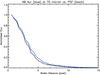 |
Fig. 1 Radial profile for AB aur in blue at 70 μm, PSF (α Boo) in black. Object emission is more extended than the emission from a point source obtained using the same observation mode and reduction procedure. This a showcase of our marginally resolved sources. |
Gaussian fit to our sample.
Three of the five HAeBe stars with spatially resolved discs have large inner gaps and prominent dust rings at distances greater than 100 au. At 1.3 mm, AB Aur has a dust ring with the peak of the dust emission at 145 au (Tang et al. 2012), HD 141569A has three major rings seen in scattered light at 15, 185, and 300 au (Clampin et al. 2003; Thi et al. 2014), while at mm wavelengths, HD 142527 has a large gap between 10 and 140 au, which contains gas but very little dust (Casassus et al. 2012). The only debris disc which we resolved, 49 Cet, is also know to have an outer disc with large grains with an inner radius of 60 au, which dominates the emission at far-infrared wavelengths (Wahhaj et al. 2007). Its disc was also resolved with PACS by Roberge et al. (2013), who did a deconvolution of their 70 μm image and found a half-width at half maximum along the disc major axis of ~200 au, consistent with measurements of the CO disc (Hughes et al. 2008), but no sign of a central clearing, likely due to the angular resolution of Herschel/PACS.
A necessary condition for seeing spatially extended far-infrared emission therefore seems to be that the disc has to have large inner gaps and dust rings at large radii, which contribute to or dominate the observed emission. This is almost certainly the case for HD 104237, which has not been studied in as much detail as the other three stars. An attempt to image the disc with the Hubble Space Telescope “Space Telescope Imaging Spectrograph” instrument was unsuccessful (Grady et al. 2004). However, high contrast imaging has advanced greatly in the past ten years, in particular the advent of high contrast, high angular resolution imaging provides exciting avenues for further exploration and characterisation of such systems. It is likely that HD 104237 will show features similar to those seen for the other three HAeBe stars resolved with PACS. Another option is to observed the star with ALMA, which has unprecedented angular resolution and sensitivity at millimetre and sub-millimetre wavelengths, tracing the largest and coldest dust grains in the circumstellar disc.
4. Discussion
In the following section we only discuss the HAeBes. We neglect the debris discs in the discussion because their discs are fundamentally different, because it is much less massive and optically thin and has rare examples of gas emission (e.g. Donaldson et al. 2013; Moór et al. 2011; Roberge et al. 2013). As previously noted in Meijer et al. (2008), there is no natural dichotomy in the appearance of the source SEDs. Rather, a smooth transition exists between group I and II sources. This is also seen in our results. However, making a distinction is a useful tool for studying the disc geometry. For each group, we have calculated the mean value of the total fractional excesses, the far-infrared excesses, the ratios FNIR/FFIR, the mm slope, and 1.3 mm flux. (see Table 6).
Mean, total, and far-infrared excess, FIR/NIR flux ratio, mm slope, mm flux, and [O i] 63 μm line flux for each group of sources.
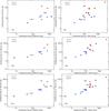 |
Fig. 2 PACS 70, 100, and 160 μm fluxes (top to bottom) plotted against sub-mm data (left hand column) and mm data (right hand column). The far-infrared correlates with the mm region with a tighter correlation for longer wavelengths. Statistical analysis is presented in Table 4. |
From the parameter study by Meijer et al. (2008) it became clear that, while the SED shortward of 60 μm is determined by the mass in small (<25 μm) dust grains, the SED longward of 100 μm is mainly determined by the larger dust grains that are located in the disc midplane. Adding larger dust grains to the disc will increase the mm flux, as well as change the slope of the mm SED. We now use our PACS photometry to study these effects in our sample of HAeBes. Therefore, we need to keep the following in mind:
-
1.
The SED classification (group I/II) is based onwavelengths up to 60 μm and isdetermined by the mass in small grains;
-
2.
The SED at λ> 100μm is determined by the larger dust grains;
-
3.
At mm wavelengths, the emission is optically thin, hence the flux relates to the total dust mass (excluding larger bodies such as pebbles);
-
4.
The slope at mm wavelengths gives an indication of grain size.
In Fig. 2 we plot the source fluxes in each PACS waveband as a function of the flux at 850 and 1300 μm. The fluxes are scaled to a distance of 140 pc to correct for distance effects. For group II sources there is a clear correlation between the far-infrared and mm fluxes, and the correlation is stronger at longer wavelengths. This means that an increase in disc mass is accompanied by an increase in far-infrared flux, as already predicted by Meijer et al. (2008), the effect being stronger at longer wavelengths, where the disc becomes more and more optically thin. It is interesting to note that the correlation is only seen for the group II sources, the flared discs do not show a correlation. This is likely due to a greater importance of their UV luminosities and PAH emission, contributing to the heating of the gas, visible at IR wavelengths (see discussion in Meeus et al. 2012).
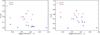 |
Fig. 3 Far-infrared (left) and infrared (right) excess versus mm continuum and slope, as shown in Table 4. Only far-infrared excess is tentatively correlated to the mm slope (plot on the left). |
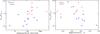 |
Fig. 4 Excess ratio versus 1.3 mm continuum flux density (left) and infrared-millimetre slope (right). There are no correlations between these parameters. |
In Fig. 3, we plot the excesses as a function of the mm slope. We do not observe a correlation, but on average, the excesses are larger for sources with steeper mm slopes (see Table 6). This indicates that a larger number of small grains (steeper slope) increases the (far-)infrared excess, confirming the prediction by Dullemond & Dominik (2004): since small grains dominate the opacity, an increase in their mass will lead to an increased amount of flaring.
In Fig. 4, we plot the excess ratio as a function of the 1.3 mm flux density and the infrared to mm slope. Here we observe the following: the ratio of far-infrared to near-infrared flux (FIR/NIR) correlates with the mm flux: flaring discs have a higher dust mass than flat discs (excluding the mass in larger grains that might be hiding in the disc midplane. The FIR/NIR ratio also tends to be larger for sources with a steeper mm slope, again indicating that an increase in lower grain mass leads to an increase in flaring.
In Fig. 5 we plot the [OI] 63 μm flux density as a function of the far- to near-IR ratio. The three sources with the highest [OI] flux densities are the FUV bright stars, AB Aur, HD 97048, and HD 100546. Excluding those three sources, there is no correlation between the [O i] 63 μm line flux density and the far-infrared to near-infrared flux ratio. On average, the group I sources do have higher [O i] 63 μm line flux density than group II sources (see Table 6).
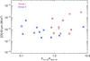 |
Fig. 5 [O i] 63 μm line flux as a function of the far-IR/near-IR ratio, where a correlation is not observed. |
5. Conclusions
In this paper, we present new Herschel/PACS far-infrared photometry and imaging observations obtained at 70 (and/or) 100, and 160 μm for a sample of 22 HAeBes and five debris discs. We combine these new measurements with literature data across a broad range of wavelengths to complement the far-infrared photometry and construct SEDs. We calculated the discs’ excesses in three regimes that span the near-, mid-, and far-infrared, as well as the total excess due to disc emission. This is the first time the group I/II discs have been studied at far-infrared wavelengths; previous studies concentrated on the SED up to 60 μm, with a comparison to the mm region. The region between 100 and 160 μm is important because it is where the disc evolves from an optically thick to an optically thin regime (see discussion in Meijer et al. 2008).
As has been previously noted (e.g. Dominik et al. 2003), group I sources have, on average, larger infrared excesses than group II sources, as well as steeper mm slopes (Acke et al. 2004). This suggests that a higher mass of small dust grains is present in these group I sources. In our observations, we observe a similar trend, including the excesses at far-infrared wavelengths. These results could be consistent with an evolution from group I to group II. However, we note that this evolutionary scenario is currently under debate (e.g. Mendigutía et al. 2012; Maaskant et al. 2013).
Relating the far-infrared emission of HAeBe discs with other observational properties, we found the following:
-
1.
For group II sources, the far-infrared fluxdensity correlates with the mm flux density, thecorrelation being stronger for longer wavelengths. This suggeststhat the emission in the far-infrared correlates with the dust mass.The far-infrared flux densities of group I sourcesdo not correlate with the corresponding mm fluxdensities and are likely more influenced by the stellar UVluminosity and heating by PAHs.
-
2.
On average, the far-infrared excess is greater for sources with steeper mm slopes: a larger number of small grains increases the far-infrared excess.
-
3.
The far-infrared to near-infrared excess ratio is greater for sources with a higher 1.3 mm flux, implying a greater degree of flaring, while the sub-mm slope is steeper for larger excess ratios.
-
4.
We do not find a correlation between the [O i] 63 μm line flux and the far-infrared to near-infrared excess ratio, but on average group I sources have higher [O i] 63 μm line fluxes.
We also studied the spatial extent of our sources in the far-infrared. Several of our sources show a larger spatial extent than expected of a point source, namely: AB Aur, HD 100546, HD 104237, HD 141569A, HD 142527, and the debris disc 49 Cet.
Finally, the photometric data set presented here is important for cross-calibrating Herschel/PACS spectra, whose absolute flux calibration is not as certain. This aspect of our work has already been presented in several papers from the GASPS consortium (e.g. Fedele et al. 2013; Meeus et al. 2013).
Acknowledgments
We would like to thank the PACS instrument team for their dedicated support and M. van den Ancker for the bibliographic photometry data. G. Meeus, J.P. Marshall, and B. Montesinos are partly supported by AYA-2011-26202. G. Meeus is supported by RYC-2011-07920. J.P. Marshall is supported by a UNSW Vice Chancellor’s Fellowship. This research made use of the SIMBAD database, operated at the CDS, Strasbourg, France.
References
- Acke, B., van den Ancker, M. E., Dullemond, C. P., van Boekel, R., & Waters, L. B. F. M. 2004, A&A, 422, 621 [NASA ADS] [CrossRef] [EDP Sciences] [Google Scholar]
- Allen, D. A. 1973, MNRAS, 161, 145 [NASA ADS] [Google Scholar]
- Andrews, S. M., Wilner, D. J., Espaillat, C., et al. 2011, ApJ, 732, 42 [NASA ADS] [CrossRef] [Google Scholar]
- Augereau, J. C., Lagrange, A. M., Mouillet, D., & Ménard, F. 2001, A&A, 365, 78 [NASA ADS] [CrossRef] [EDP Sciences] [Google Scholar]
- Baines, D., Oudmaijer, R. D., Porter, J. M., & Pozzo, M. 2006, MNRAS, 367, 737 [NASA ADS] [CrossRef] [MathSciNet] [Google Scholar]
- Balog, Z., Müller, T., Nielbock, M., et al. 2014, Exper. Astron., 37, 129 [NASA ADS] [CrossRef] [Google Scholar]
- Banzatti, A., Testi, L., Isella, A., et al. 2011, A&A, 525, A12 [NASA ADS] [CrossRef] [EDP Sciences] [Google Scholar]
- Berrilli, F., Corciulo, G., Ingrosso, G., et al. 1992, ApJ, 398, 254 [NASA ADS] [CrossRef] [Google Scholar]
- Beskrovnaya, N. G., Pogodin, M. A., Miroshnichenko, A. S., et al. 1999, A&A, 343, 163 [NASA ADS] [Google Scholar]
- Biller, B., Lacour, S., Juhász, A., et al. 2012, ApJ, 753, L38 [NASA ADS] [CrossRef] [Google Scholar]
- Blondel, P. F. C., & Djie, H. R. E. T. A. 2006, A&A, 456, 1045 [NASA ADS] [CrossRef] [EDP Sciences] [Google Scholar]
- Bross, I. D. J. 1971, in Foundations of Statistical Inference, eds. V. P. Godambe, & Sprott (Toronto: Holt, Rinehart & Winston of Canada, Ltd.) [Google Scholar]
- Brott, I., & Hauschildt, P. H. 2005, in The Three-Dimensional Universe with Gaia, eds. C. Turon, K. S. O’Flaherty, & M. A. C. Perryman, ESA SP, 576, 565 [Google Scholar]
- Casassus, S., Perez, M. S., Jordán, A., et al. 2012, ApJ, 754, L31 [NASA ADS] [CrossRef] [Google Scholar]
- Chen, X. P., Henning, T., van Boekel, R., & Grady, C. A. 2006, A&A, 445, 331 [NASA ADS] [CrossRef] [EDP Sciences] [Google Scholar]
- Chiang, E. I., Joung, M. K., Creech-Eakman, M. J., et al. 2001, ApJ, 547, 1077 [NASA ADS] [CrossRef] [Google Scholar]
- Clampin, M., Krist, J. E., Ardila, D. R., et al. 2003, AJ, 126, 385 [NASA ADS] [CrossRef] [Google Scholar]
- Close, L. M., Follette, K. B., Males, J. R., et al. 2014, ApJ, 781, L30 [NASA ADS] [CrossRef] [Google Scholar]
- Cohen, M., & Schwartz, R. D. 1976, MNRAS, 174, 137 [NASA ADS] [CrossRef] [Google Scholar]
- Coulson, I. M., & Walther, D. M. 1995, MNRAS, 274, 977 [NASA ADS] [Google Scholar]
- Davies, J. K., Evans, A., Bode, M. F., & Whittet, D. C. B. 1990, MNRAS, 247, 517 [NASA ADS] [Google Scholar]
- de Winter, D., van den Ancker, M. E., Maira, A., et al. 2001, A&A, 380, 609 [NASA ADS] [CrossRef] [EDP Sciences] [Google Scholar]
- Dent, W. R. F., Thi, W. F., Kamp, I., et al. 2013, PASP, 125, 477 [NASA ADS] [CrossRef] [Google Scholar]
- Dominik, C., Dullemond, C. P., Waters, L. B. F. M., & Walch, S. 2003, A&A, 398, 607 [NASA ADS] [CrossRef] [EDP Sciences] [Google Scholar]
- Donaldson, J. K., Lebreton, J., Roberge, A., Augereau, J.-C., & Krivov, A. V. 2013, ApJ, 772, 17 [NASA ADS] [CrossRef] [Google Scholar]
- Dong, Y.-S., & Hu, J.-Y. 1991, Acta Astrophysica Sinica, 11, 172 [Google Scholar]
- Dullemond, C. P., & Dominik, C. 2004, A&A, 421, 1075 [NASA ADS] [CrossRef] [EDP Sciences] [Google Scholar]
- Dunkin, S. K., & Crawford, I. A. 1998, MNRAS, 298, 275 [NASA ADS] [CrossRef] [Google Scholar]
- Eiroa, C., Garzón, F., Alberdi, A., et al. 2001, A&A, 365, 110 [NASA ADS] [CrossRef] [EDP Sciences] [Google Scholar]
- Fajardo-Acosta, S. B., Telesco, C. M., & Knacke, R. F. 1998, AJ, 115, 2101 [NASA ADS] [CrossRef] [Google Scholar]
- Fedele, D., Bruderer, S., van Dishoeck, E. F., et al. 2013, A&A, 559, A77 [NASA ADS] [CrossRef] [EDP Sciences] [Google Scholar]
- Feigelson, E. D., Lawson, W. A., & Garmire, G. P. 2003, ApJ, 599, 1207 [NASA ADS] [CrossRef] [Google Scholar]
- Fouque, P., Le Bertre, T., Epchtein, N., Guglielmo, F., & Kerschbaum, F. 1992, A&AS, 93, 151 [NASA ADS] [Google Scholar]
- Garcia, P. J. V., Benisty, M., Dougados, C., et al. 2013, MNRAS, 430, 1839 [NASA ADS] [CrossRef] [Google Scholar]
- Garcia Lopez, R., Natta, A., Testi, L., & Habart, E. 2006, A&A, 459, 837 [NASA ADS] [CrossRef] [EDP Sciences] [Google Scholar]
- Garufi, A., Quanz, S. P., Avenhaus, H., et al. 2013, A&A, 560, A105 [NASA ADS] [CrossRef] [EDP Sciences] [Google Scholar]
- Grady, C. A., Woodgate, B., Torres, C. A. O., et al. 2004, ApJ, 608, 809 [NASA ADS] [CrossRef] [Google Scholar]
- Grady, C. A., Schneider, G., Sitko, M. L., et al. 2009, ApJ, 699, 1822 [NASA ADS] [CrossRef] [Google Scholar]
- Guilloteau, S., Dutrey, A., Piétu, V., & Boehler, Y. 2011, A&A, 529, A105 [NASA ADS] [CrossRef] [EDP Sciences] [Google Scholar]
- Harmanec, P., & Božić, H. 2001, A&A, 369, 1140 [NASA ADS] [CrossRef] [EDP Sciences] [Google Scholar]
- Hauck, B., & Mermilliod, M. 1998, A&AS, 129, 431 [NASA ADS] [CrossRef] [EDP Sciences] [Google Scholar]
- Henning, T., Pfau, W., Zinnecker, H., & Prusti, T. 1993, A&A, 276, 129 [NASA ADS] [Google Scholar]
- Henning, T., Launhardt, R., Steinacker, J., & Thamm, E. 1994, A&A, 291, 546 [NASA ADS] [Google Scholar]
- Herbig, G. H. 1960, ApJS, 4, 337 [NASA ADS] [CrossRef] [Google Scholar]
- Hillenbrand, L. A., Strom, S. E., Vrba, F. J., & Keene, J. 1992, ApJ, 397, 613 [NASA ADS] [CrossRef] [Google Scholar]
- Houck, J. R., Roellig, T. L., van Cleve, J., et al. 2004, ApJS, 154, 18 [NASA ADS] [CrossRef] [Google Scholar]
- Hu, J. Y., The, P. S., & de Winter, D. 1989, A&A, 208, 213 [NASA ADS] [Google Scholar]
- Hughes, A. M., Wilner, D. J., Kamp, I., & Hogerheijde, M. R. 2008, ApJ, 681, 626 [NASA ADS] [CrossRef] [Google Scholar]
- Hutchinson, M. G., Albinson, J. S., Barrett, P., et al. 1994, A&A, 285, 883 [NASA ADS] [Google Scholar]
- Jensen, E. L. N., Mathieu, R. D., & Fuller, G. A. 1996, ApJ, 458, 312 [Google Scholar]
- Juhász, A., Bouwman, J., Henning, T., et al. 2010, ApJ, 721, 431 [NASA ADS] [CrossRef] [Google Scholar]
- Kamp, I., & Dullemond, C. P. 2004, ApJ, 615, 991 [NASA ADS] [CrossRef] [Google Scholar]
- Kessler, M. F., Steinz, J. A., Anderegg, M. E., et al. 1996, A&A, 315, L27 [NASA ADS] [Google Scholar]
- Kilkenny, D., Whittet, D. C. B., Davies, J. K., et al. 1985, South African Astronomical Observatory Circular, 9, 55 [Google Scholar]
- Kraus, S., Hofmann, K.-H., Benisty, M., et al. 2008, A&A, 489, 1157 [NASA ADS] [CrossRef] [EDP Sciences] [Google Scholar]
- Lawrence, G., Jones, T. J., & Gehrz, R. D. 1990, AJ, 99, 1232 [NASA ADS] [CrossRef] [Google Scholar]
- Low, F. J., Smith, P. S., Werner, M., et al. 2005, ApJ, 631, 1170 [NASA ADS] [CrossRef] [Google Scholar]
- Lyo, A.-R., Ohashi, N., Qi, C., Wilner, D. J., & Su, Y.-N. 2011, AJ, 142, 151 [NASA ADS] [CrossRef] [Google Scholar]
- Maaskant, K. M., Honda, M., Waters, L. B. F. M., et al. 2013, A&A, 555, A64 [NASA ADS] [CrossRef] [EDP Sciences] [Google Scholar]
- Malfait, K., Bogaert, E., & Waelkens, C. 1998, A&A, 331, 211 [NASA ADS] [Google Scholar]
- Mannings, V. 1994, MNRAS, 271, 587 [NASA ADS] [Google Scholar]
- Mannings, V., & Sargent, A. I. 1997, ApJ, 490, 792 [NASA ADS] [CrossRef] [Google Scholar]
- Mannings, V., & Sargent, A. I. 2000, ApJ, 529, 391 [NASA ADS] [CrossRef] [Google Scholar]
- Manoj, P., Bhatt, H. C., Maheswar, G., & Muneer, S. 2006, ApJ, 653, 657 [NASA ADS] [CrossRef] [Google Scholar]
- Meeus, G., Waters, L. B. F. M., Bouwman, J., et al. 2001, A&A, 365, 476 [NASA ADS] [CrossRef] [EDP Sciences] [Google Scholar]
- Meeus, G., Montesinos, B., Mendigutía, I., et al. 2012, A&A, 544, A78 [NASA ADS] [CrossRef] [EDP Sciences] [Google Scholar]
- Meeus, G., Salyk, C., Bruderer, S., et al. 2013, A&A, 559, A84 [NASA ADS] [CrossRef] [EDP Sciences] [Google Scholar]
- Meijer, J., Dominik, C., de Koter, A., et al. 2008, A&A, 492, 451 [NASA ADS] [CrossRef] [EDP Sciences] [Google Scholar]
- Mendigutía, I., Mora, A., Montesinos, B., et al. 2012, A&A, 543, A59 [NASA ADS] [CrossRef] [EDP Sciences] [Google Scholar]
- Mendigutía, I., Fairlamb, J., Montesinos, B., et al. 2014, ApJ, 790, 21 [NASA ADS] [CrossRef] [Google Scholar]
- Miroshnichenko, A. S., Mulliss, C. L., Bjorkman, K. S., et al. 1999, MNRAS, 302, 612 [NASA ADS] [CrossRef] [Google Scholar]
- Moerchen, M. M., Telesco, C. M., Packham, C., & Kehoe, T. J. J. 2007, ApJ, 655, L109 [NASA ADS] [CrossRef] [Google Scholar]
- Montesinos, B., Eiroa, C., Mora, A., & Merín, B. 2009, A&A, 495, 901 [NASA ADS] [CrossRef] [EDP Sciences] [Google Scholar]
- Moór, A., Ábrahám, P., Juhász, A., et al. 2011, ApJ, 740, L7 [NASA ADS] [CrossRef] [Google Scholar]
- Müller, A., van den Ancker, M. E., Launhardt, R., et al. 2011, A&A, 530, A85 [NASA ADS] [CrossRef] [EDP Sciences] [Google Scholar]
- Neugebauer, G., Habing, H. J., van Duinen, R., et al. 1984, ApJ, 278, L1 [Google Scholar]
- Ott, S. 2010, in Astronomical Data Analysis Software and Systems XIX, eds. Y. Mizumoto, K.-I. Morita, & M. Ohishi, ASP Conf. Ser., 434, 139 [Google Scholar]
- Oudmaijer, R. D., van der Veen, W. E. C. J., Waters, L. B. F. M., et al. 1992, A&AS, 96, 625 [NASA ADS] [Google Scholar]
- Oudmaijer, R. D., Palacios, J., Eiroa, C., et al. 2001, A&A, 379, 564 [NASA ADS] [CrossRef] [EDP Sciences] [Google Scholar]
- Pilbratt, G. L., Riedinger, J. R., Passvogel, T., et al. 2010, A&A, 518, L1 [CrossRef] [EDP Sciences] [Google Scholar]
- Poglitsch, A., Waelkens, C., Geis, N., et al. 2010, A&A, 518, L2 [NASA ADS] [CrossRef] [EDP Sciences] [Google Scholar]
- Preibisch, T., Kraus, S., Driebe, T., van Boekel, R., & Weigelt, G. 2006, A&A, 458, 235 [NASA ADS] [CrossRef] [EDP Sciences] [Google Scholar]
- Raman, A., Lisanti, M., Wilner, D. J., Qi, C., & Hogerheijde, M. 2006, AJ, 131, 2290 [NASA ADS] [CrossRef] [Google Scholar]
- Roberge, A., & Weinberger, A. J. 2008, ApJ, 676, 509 [NASA ADS] [CrossRef] [Google Scholar]
- Roberge, A., Kamp, I., Montesinos, B., et al. 2013, ApJ, 771, 69 [NASA ADS] [CrossRef] [Google Scholar]
- Sandell, G., Weintraub, D. A., & Hamidouche, M. 2011, ApJ, 731, 133 [NASA ADS] [CrossRef] [Google Scholar]
- Shenavrin, V. I., Grinin, V. P., Rostopchina-Shakhovskaja, A. N., Demidova, T. V., & Shakhovskoi, D. N. 2012, Astron. Rep., 56, 379 [NASA ADS] [CrossRef] [Google Scholar]
- Sheret, I., Dent, W. R. F., & Wyatt, M. C. 2004, MNRAS, 348, 1282 [NASA ADS] [CrossRef] [Google Scholar]
- Sitko, M. L., Carpenter, W. J., Kimes, R. L., et al. 2008, ApJ, 678, 1070 [NASA ADS] [CrossRef] [Google Scholar]
- Stauffer, J. R., Hartmann, L. W., & Barrado y Navascues, D. 1995, ApJ, 454, 910 [NASA ADS] [CrossRef] [Google Scholar]
- Stecklum, B., Eckart, A., Henning, T., & Loewe, M. 1995, A&A, 296, 463 [NASA ADS] [Google Scholar]
- Su, K. Y. L., Rieke, G. H., Stansberry, J. A., et al. 2006, ApJ, 653, 675 [NASA ADS] [CrossRef] [Google Scholar]
- Sylvester, R. J., Skinner, C. J., Barlow, M. J., & Mannings, V. 1996, MNRAS, 279, 915 [NASA ADS] [CrossRef] [Google Scholar]
- Tang, Y.-W., Guilloteau, S., Piétu, V., et al. 2012, A&A, 547, A84 [NASA ADS] [CrossRef] [EDP Sciences] [Google Scholar]
- Testi, L., Natta, A., Shepherd, D. S., & Wilner, D. J. 2001, ApJ, 554, 1087 [Google Scholar]
- The, P. S., Tjin-A-Djie, H. R. E., Bakker, R., et al. 1981, A&AS, 44, 451 [NASA ADS] [Google Scholar]
- The, P. S., Cuypers, H., Tjin A Djie, H. R. E., & Felenbok, P. 1985, A&A, 149, 429 [NASA ADS] [Google Scholar]
- The, P. S., Wesselius, P. R., & Janssen, I. M. H. H. 1986, A&AS, 66, 63 [NASA ADS] [Google Scholar]
- The, P. S., de Winter, D., & Perez, M. R. 1994, A&AS, 104, 315 [NASA ADS] [Google Scholar]
- Thi, W.-F., Pinte, C., Pantin, E., et al. 2014, A&A, 561, A50 [NASA ADS] [CrossRef] [EDP Sciences] [Google Scholar]
- Thomas, S. J., van der Bliek, N. S., Rodgers, B., Doppmann, G., & Bouvier, J. 2007, in IAU Symp. 240, eds. W. I. Hartkopf, P. Harmanec, & E. F. Guinan, 250 [Google Scholar]
- van Boekel, R., Waters, L. B. F. M., Dominik, C., et al. 2003, A&A, 400, L21 [NASA ADS] [CrossRef] [EDP Sciences] [Google Scholar]
- van Boekel, R., Min, M., Waters, L. B. F. M., et al. 2005, A&A, 437, 189 [NASA ADS] [CrossRef] [EDP Sciences] [Google Scholar]
- van den Ancker, M. E., de Winter, D., & Tjin A Djie, H. R. E. 1998, A&A, 330, 145 [NASA ADS] [Google Scholar]
- van der Veen, W. E. C. J., Habing, H. J., & Geballe, T. R. 1989, A&A, 226, 108 [NASA ADS] [Google Scholar]
- van Leeuwen, F. 2007, A&A, 474, 653 [NASA ADS] [CrossRef] [EDP Sciences] [Google Scholar]
- Wahhaj, Z., Koerner, D. W., & Sargent, A. I. 2007, ApJ, 661, 368 [NASA ADS] [CrossRef] [Google Scholar]
- Walker, H. J., & Butner, H. M. 1995, Ap&SS, 224, 389 [NASA ADS] [CrossRef] [Google Scholar]
- Waters, L. B. F. M., & Waelkens, C. 1998, ARA&A, 36, 233 [NASA ADS] [CrossRef] [Google Scholar]
- Waters, L. B. F. M., Cote, J., & Geballe, T. R. 1988, A&A, 203, 348 [NASA ADS] [Google Scholar]
- Weaver, W. B., & Jones, G. 1992, ApJS, 78, 239 [NASA ADS] [CrossRef] [Google Scholar]
- Weinberger, A. J., Rich, R. M., Becklin, E. E., Zuckerman, B., & Matthews, K. 2000, ApJ, 544, 937 [NASA ADS] [CrossRef] [Google Scholar]
- Werner, M. W., Roellig, T. L., Low, F. J., et al. 2004, ApJS, 154, 1 [Google Scholar]
- Wheelwright, H. E., Oudmaijer, R. D., & Goodwin, S. P. 2010, MNRAS, 401, 1199 [NASA ADS] [CrossRef] [Google Scholar]
- Williams, J. P., & Cieza, L. A. 2011, ARA&A, 49, 67 [NASA ADS] [CrossRef] [Google Scholar]
- Zuckerman, B., & Song, I. 2012, ApJ, 758, 77 [NASA ADS] [CrossRef] [Google Scholar]
Appendix A: SEDs
In Figs. A.1 and A.2 we show the spectral energy distributions of the objects studied in this paper. The red triangles show the PACS fluxes, red arrows are 3σ upper limits. The literature data used to build the SED are plotted as blue circles. When available, the IUE spectrum is plotted as a solid dark red line and the Spitzer/IRS spectrum as a purple line. The solid black line is the PHOENIX/Gaia model fitted to the stellar photospheric emission. Table A.2 gives the references for the photometry collected to build the SEDs.
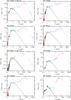 |
Fig. A.1 SEDs of GASPS Herbig Ae/Be stars. PACS fluxes reported in this work can be identified with red triangles. Red arrows are 3σ upper limits. Blue circles correspond to literature data from Table A.2. The solid dark red line shows IUE spectrum and purple line for the Spitzer/IRS spectrum. The solid black line is the PHOENIX/Gaia model fitted to the stellar photospheric emission. |
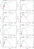 |
Fig. A.1 SEDs of GASPS Herbig Ae/Be stars (continued). |
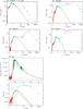 |
Fig. A.1 SEDs of GASPS Herbig Ae/Be stars (continued). The KK Oph fit was made manually and is shown in two wavelength intervals: 0.1−2.3 μm and 0.1−4000 μm. The models for the cool and hot components are in red and green, respectively, shown scaled according to their spectral types and luminosity classes. With only five photometry points in the optical, it was assumed that the contribution to the UV U and B flux comes mostly from the hot component, and the extinction was adjusted for this component. Then, the model for the cool component was reddened with different amounts of AV until the total flux at V and R was matched by sum of the models of the hot and cool components (both of them reddened); the final composite model is shown in black. |
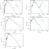 |
Fig. A.2 SEDs of GASPS debris-disc host stars. |
Reddening values applied to the stellar atmosphere models in order to fit them to the optical photometry available, RV = 3.1 is assumed.
References used for the construction of the SEDs.
Appendix B: PACS observation identifications
In Table B.1 we present the Herschel/PACS observation log, listing the observation IDs and integration times and observation dates for every target in our sample. Concatenated scan pairs (or quartets) are denoted by a “/” between numbers at the end of the observation ID, whilst distinct observations of the same target are separated by a “,”.
Observation log.
Appendix C: Extended sources profiles
As previously shown for AB Aur, here we present plots of the radial profiles of our extended sources compared to the radial profile of the point source α Boo.
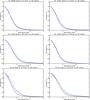 |
Fig. C.1 Radial profiles for extended sources compared with a discless point source. One pixel is equivalent to 1′′. |
All Tables
Photometry measured for the sample, taking the colour and aperture corrections into account.
Wavelength λ0 at which the excess starts in the target SED and the fractional excesses in the near-, mid-, and far-infrared.
Mean, total, and far-infrared excess, FIR/NIR flux ratio, mm slope, mm flux, and [O i] 63 μm line flux for each group of sources.
Reddening values applied to the stellar atmosphere models in order to fit them to the optical photometry available, RV = 3.1 is assumed.
All Figures
|
Fig. 1 Radial profile for AB aur in blue at 70 μm, PSF (α Boo) in black. Object emission is more extended than the emission from a point source obtained using the same observation mode and reduction procedure. This a showcase of our marginally resolved sources. |
| In the text | |
|
Fig. 2 PACS 70, 100, and 160 μm fluxes (top to bottom) plotted against sub-mm data (left hand column) and mm data (right hand column). The far-infrared correlates with the mm region with a tighter correlation for longer wavelengths. Statistical analysis is presented in Table 4. |
| In the text | |
|
Fig. 3 Far-infrared (left) and infrared (right) excess versus mm continuum and slope, as shown in Table 4. Only far-infrared excess is tentatively correlated to the mm slope (plot on the left). |
| In the text | |
|
Fig. 4 Excess ratio versus 1.3 mm continuum flux density (left) and infrared-millimetre slope (right). There are no correlations between these parameters. |
| In the text | |
|
Fig. 5 [O i] 63 μm line flux as a function of the far-IR/near-IR ratio, where a correlation is not observed. |
| In the text | |
|
Fig. A.1 SEDs of GASPS Herbig Ae/Be stars. PACS fluxes reported in this work can be identified with red triangles. Red arrows are 3σ upper limits. Blue circles correspond to literature data from Table A.2. The solid dark red line shows IUE spectrum and purple line for the Spitzer/IRS spectrum. The solid black line is the PHOENIX/Gaia model fitted to the stellar photospheric emission. |
| In the text | |
|
Fig. A.1 SEDs of GASPS Herbig Ae/Be stars (continued). |
| In the text | |
|
Fig. A.1 SEDs of GASPS Herbig Ae/Be stars (continued). The KK Oph fit was made manually and is shown in two wavelength intervals: 0.1−2.3 μm and 0.1−4000 μm. The models for the cool and hot components are in red and green, respectively, shown scaled according to their spectral types and luminosity classes. With only five photometry points in the optical, it was assumed that the contribution to the UV U and B flux comes mostly from the hot component, and the extinction was adjusted for this component. Then, the model for the cool component was reddened with different amounts of AV until the total flux at V and R was matched by sum of the models of the hot and cool components (both of them reddened); the final composite model is shown in black. |
| In the text | |
|
Fig. A.2 SEDs of GASPS debris-disc host stars. |
| In the text | |
|
Fig. C.1 Radial profiles for extended sources compared with a discless point source. One pixel is equivalent to 1′′. |
| In the text | |
Current usage metrics show cumulative count of Article Views (full-text article views including HTML views, PDF and ePub downloads, according to the available data) and Abstracts Views on Vision4Press platform.
Data correspond to usage on the plateform after 2015. The current usage metrics is available 48-96 hours after online publication and is updated daily on week days.
Initial download of the metrics may take a while.