© ESO, 2016

1. Introduction

In a series of previous papers (Buldgen et al. 2015b,a), we analysed the theoretical aspects of the use of seismic inversion techniques to characterise extra mixing in stellar interiors. Instead of trying to determine entire structural profiles, as was successfully done in helioseismology (Basu et al. 1997, 1996; Basu & Christensen-Dalsgaard 1997; see also Christensen-Dalsgaard 2002 for an extensive review on helioseismology), we make use of multiple indicators, defined as integrated quantities which are sensitive to various effects in the structure. These indicators are ultimately new seismic constraints using all the available information provided by the pulsation frequencies.

In this paper, we apply our method to the binary system 16Cyg, which was observed by Kepler, for which data of unprecedented quality is available. Moreover, this system has already been extensively studied, particularly since the discovery of a red dwarf and a Jovian planet in it (see Cochran et al. 1997). Using Kepler data, this system has been further constrained by asteroseismic studies (Metcalfe et al. 2012; Gruberbauer et al. 2013; Mathur et al. 2012), interferometric radii have also been determined (see White et al. 2013) and more recently, Verma et al. have determined the surface helium abundance (Verma et al. 2014) of both stars and Davies et al. (2015) analysed their rotation profiles and tested gyrochronologic relations for this system.

The excellent quality of the Kepler data for these stars enables us to use our inversion technique to constrain their structure. We use the previous studies as a starting point and determine the stellar parameters using spectroscopic constraints from Ramírez et al. (2009) and Tucci Maia et al. (2014), the surface helium constraints from Verma et al. (2014) and the frequencies from the full length of the Kepler mission used in Davies et al. (2015) and check for consistency with the interferometric radius from White et al. (2013). The determination of the stellar model parameters is described in Sect. 2. We carry out a first modelling process then determine the acoustic radius and the mean density using the SOLA technique (Pijpers & Thompson 1994) adapted to the determination of these integrated quantities (see Buldgen et al. 2015b; Reese et al. 2012). In Sect. 3, we briefly recall the definition and purpose of the indicator t_u and carry out inversions of this indicator for both stars. We then discuss the accuracy of these results. Finally, in Sect. 4, we use the knowledge obtained from the inversion technique to provide additional and less model-dependent constraints on the chemical composition and microscopic diffusion in 16CygA. These constraints on the chemical and atomic diffusion properties allow us to provide accurate, yet of course model-dependent, ages for this system, using the most recent observational data. The philosophy behind our study matches the so-called “à la carte” asteroseismology of Lebreton & Goupil (2012) for HD52265, where one wishes to test the physics of the models and quantify the consequences of these changes. However, we add a substantial qualitative step by supplementing the classical seismic analysis with inversion techniques.

2. Determination of the reference model parameters

2.1. Initial fits and impact of diffusion processes

In this section, we describe the optimization process that led to the reference models for the inversions. We carried out an independent seismic modelling of both stars using the frequency spectrum from Davies et al. (2015), which was based on 928 days of Kepler data. A Levenberg-Marquardt algorithm was used to determine the optimal set of free parameters for our models. We used the Clés stellar evolution code and the Losc oscillation code (Scuflaire et al. 2008b,a) to build the models and calculate their oscillation frequencies. We used the CEFF equation of state (Christensen-Dalsgaard & Daeppen 1992), the OPAL opacities from Iglesias & Rogers (1996), supplemented at low temperature by the opacities of Ferguson et al. (2005) and the effects of conductivity from Potekhin et al. (1999) and Cassisi et al. (2007). The nuclear reaction rates we used are those from the NACRE project (Angulo et al. 1999), supplemented by the updated reaction rate from Formicola et al. (2004) and convection was implemented using the classical, local mixing-length theory (Böhm-Vitense 1958). We also used the implementation of microscopic diffusion from Thoul et al. (1994), for which three groups of elements are considered and treated separately: hydrogen, helium and the metals (all considered to have diffusion speeds of ⁵⁶Fe). No turbulent diffusion, penetrative convection and rotational effects have been included in the models. The empirical surface correction from Kjeldsen et al. (2008) was not used in this study. The following cost function was used when carrying out the minimization: $\begin{array}{ccc}\mathrm{𝒥}\mathrm{=}\frac{\mathrm{1}}{\mathit{N}\mathrm{-}\mathit{M}}\sum _{\mathit{i}}^{\mathit{N}}\frac{{\mathrm{(}{\mathit{A}}_{\mathrm{obs}}^{\mathit{i}}\mathrm{-}{{\mathit{A}}_{\mathrm{theo}}^{\mathit{i}}}^{\mathrm{)}}}^{\mathrm{2}}}{{\mathit{\sigma }}_{\mathit{i}}^{\mathrm{2}}}\mathit{,}& & \end{array}$(1)where ${\mathit{A}}_{\mathrm{obs}}^{\mathit{i}}$ is an observational constraint (such as individual frequencies or frequency separation, average values thereof, etc.), ${\mathit{A}}_{\mathrm{theo}}^{\mathit{i}}$ the same quantity generated from the theoretical model, σ_i is the observational error bar associated with the quantity ${\mathit{A}}_{\mathrm{obs}}^{\mathit{i}}$, N the number of observational constraints, and M the number of free parameters used to define the model. We can already comment on the use of the Levenberg-Marquardt algorithm, which is inherently a local minimization algorithm, strongly dependent on the initial values. In the following section, particular care was taken to mitigate the local character of the results since at least 35 models were computed independently for each star, using various observational constraints and initial parameter values. As far as the error bars are concerned, we looked at the scatter of the results with changes in the physical ingredients rather than the errors given by the Levenberg-Marquardt algorithm. The constraints vary according to the following two cases:

• 1.

  The model does not include any microscopic diffusion: we used the individual small frequency separations, the average large frequency separation and the effective temperature as A_i for the cost function. The chemical composition was fixed to the values given by Verma et al. (2014) and Ramírez et al. (2009). The fit used three free parameters since the chemical composition is fixed: the mixing-length parameter, denoted α_MLT, the mass and the age.

• 2.

  The model includes microscopic diffusion: we used the individual small frequency separations, the average large frequency separation, the effective temperature, the surface helium and surface metallicity constraints in the cost-function¹. We used five free parameters: the mixing-length parameter, α_MLT, the mass, the age, the initial hydrogen abundance, X₀ and the initial metallicity, Z₀.

In the case of the additional fits described in Sect. 2.3, we simply replaced the average large frequency separation by the mean density and the acoustic radius τ, thus increasing by one the number of constraints used in the cost function .

We wish to emphasize that the use of other algorithms to select a reference model does not reduce the diagnostic potential of the inversions we describe in the next sections. Indeed, inversions take a qualitative step beyond forward-modelling techniques in the sense that they explore solutions outside of the initial model parameter space.

We used various seismic and non-seismic constraints in our selection process and focussed our study on the importance of the chemical constraints for these stars. Indeed, there is a small discrepancy in the literature. In Verma et al. (2014), a less model-dependent glitch-fitting technique was used to determine the surface helium mass fraction, Y_f. It was found to be between 0.23 and 0.25 for 16CygA and between 0.218 and 0.26 for 16CygB (implying an initial helium abundance, Y₀, between 0.28 and 0.31, provided atomic diffusion is acting). In the seismic study of Metcalfe et al. (2012), various evolutionary codes and optimization processes were used and the initial helium abundance was 0.25 ± 0.01 for a model that includes microscopic diffusion. In fact, the seismic study of Gruberbauer et al. (2013) already concluded that the initial helium mass fraction had to be higher than the values provided by Metcalfe et al. (2012), which could result from the fact that they used three months of Kepler data for their study. Therefore, the starting point of our analysis was to obtain a seismic model consistent with the surface helium constraint from Verma et al. (2014) and the metallicity constraint from Ramírez et al. (2009). We started by searching for a model without including microscopic diffusion, and therefore the final surface abundances Y_f and Z_f are equal to the initial abundances Y₀ and Z₀. The metallicity can be determined using the following equation: $\begin{array}{ccc}\left[\frac{\mathrm{Fe}}{\mathrm{H}}\right]\mathrm{=}\log \left(\frac{\mathit{Z}}{\mathit{X}}\right)\mathrm{-}\log {\left(\frac{\mathit{Z}}{\mathit{X}}\right)}_{\mathrm{\odot }}\mathit{,}& & \end{array}$(2)where ${{}^{\mathrm{\right(}}\frac{\mathit{Z}}{\mathit{X}}^{\mathrm{\left)}}}_{\mathrm{\odot }}$ is the solar value consistent with the abundances used in the spectroscopic differential analysis. We point out that in the spectroscopic study of Ramírez et al. (2009), the “solar” references were the asteroids Cérès and Vesta. Their study is thus fully differential and does not depend on solar abundance results. In this study, we used the ${{}^{\mathrm{\right(}}\frac{\mathit{Z}}{\mathit{X}}^{\mathrm{\left)}}}_{\mathrm{\odot }}$ value from AGSS09 (Asplund et al. 2009) to determine the value of the metallicity Z. From the error bars provided on these chemical constraints, we can determine a two-dimensional box for the final surface chemical composition of the model (which is the initial chemical composition if the model does not include any extra mixing). A summary of the observed properties for both components is presented in Table 1. The quality of the seismic data is such that we have 54 and 56 individual frequencies for 16CygA and 16CygB respectively, determined with very high precision (typical uncertainties of 0.15 μHz). The uncertainties on the constraints in Table 1 were treated as allowed ranges for the model parameters and checked for consistency for each model we built.

An initial reference model without microscopic diffusion was obtained using the effective temperature, T_eff, the arithmetic average of the large frequency separation ⟨ Δν ⟩, and the individual small frequency separations δν_n,l. We did not include individual large frequency separations because these quantities are sensitive to surface effects in the frequencies and they would have dominated our cost function. This would have been unfortunate since we want to focus our analysis on core regions. As we see from Table 2, the model S_A,1 was also able to fit constraints such as the interferometric radius from White et al. (2013) and the luminosity from Metcalfe et al. (2012) although these quantities were not included in the of the original fit. The agreement between the observed and theoretical seismic constraints is illustrated in Fig. 1.

These results might seem correct, but since we did not even include microscopic diffusion, we should consider this model as rather unrealistic in terms of mixing processes². Therefore, we computed a few supplementary models assuming a final surface chemical composition of Y_f = 0.24 and ${{}^{\mathrm{\right(}}\frac{\mathit{Z}}{\mathit{X}}^{\mathrm{\left)}}}_{\mathit{f}}\mathrm{=}\mathrm{0.0222}$ which included microscopic diffusion following the prescriptions of Thoul et al. (1994). In this case, the fit was carried out using five free parameters, the mass, the age, the mixing length parameter, α_MLT, the initial hydrogen abundance, X₀ and the initial metallicity, Z₀. We used the same constraints as for the first fit without diffusion, supplemented by the constraints on the surface chemical composition, Y_f and (Z/X)_f providing direct and strong constraints on the initial chemical composition.

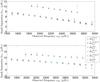Fig. 1 Upper panel: fits of the small frequency separations $\begin{array}{c}{\mathrm{˜}}_{}\\ {\mathit{\delta }}_{\mathrm{02}}\end{array}$ and $\begin{array}{c}{\mathrm{˜}}_{}\\ {\mathit{\delta }}_{\mathrm{13}}\end{array}$ for 16CygA. Lower panel: same as the upper panel for 16CygB. The observational values are the green symbols with error bars, the red symbols are associated with models including solar-calibrated diffusion and the blue symbols are associated with models without diffusion.

The effect of diffusion was mainly to reduce the mass, age and radius of the model, as illustrated in Fig. 2. This plot illustrates the effects of diffusion for various chemical compositions and diffusion velocities. The subscripts 0.0, 1.0, 0.5 are respectively related to a model without diffusion, with standard diffusion velocities and with half of these velocity values. We denote this factor D in the tables presenting the results. Each colour is associated with a particular surface chemical composition of these stars. All these models were fitted using the method described previously, and thus are compatible with all constraints that can be found in the literature for 16CygA. Therefore, the effect observed here is related to the impact of diffusion for a given model associated with a given set of frequencies. It is obvious that the reductions of the mass and radius are correlated since the mean density is kept nearly constant through the fit of the average large frequency separation. Therefore, the conclusion of this preliminary modelling process is that we obtain a degeneracy, meaning that we could build a whole family of acceptable models, inside the box of the chemical composition, with or without diffusion. This implies important uncertainties on the fundamental properties, as can be seen from the simple example in Fig. 2 for 16CygA. In the following section, we see how the use of inversion techniques and especially the inversion of t_u can help us reduce this scatter and restrict our uncertainties on fundamental properties.

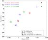Fig. 2 Effect of the progressive inclusion of diffusion in a model of 16CygA. Each model still fits the observational constraints.

Even when considering diffusion based on the work of Thoul et al. (1994), one should note that the diffusion velocities are said to be around 15−20% accurate for solar conditions. Therefore, in the particular case of 16CygA, for which we have strong constraints on the chemical composition, one can still only say that the mass has to be between 0.97 M_⊙ and 1.07 M_⊙, that the radius has to be between 1.185 R_⊙ and 1.230 R_⊙ and that the age has to be between 6.8Gy and 8.3Gy for this star. In other words, we have a ±5% mass uncertainty, ±3% radius uncertainty and ± 8% age uncertainty.

2.2. Inversion of acoustic radii and mean densities

In this section, we briefly present our results for the inversion of the mean density and the acoustic radius. The technical aspects of the inversions have been described in previous papers (see for example Reese et al. 2012; Buldgen et al. 2015b,a) but we recall them briefly at the beginning of Sect. 3. First, we note that the inverted results for the mean density and the acoustic radius are slightly different. There is a scatter of around 0.5% for both and τ depending on the reference model used for the inversion. We therefore consider that the results are τ_A = 4593 ± 15 s and g/cm³ to be consistent with the scatter we observe. For 16CygB, we obtain similar results, namely τ_B = 4066 ± 15 s and g/cm³. The kernels are well fitted, as can be seen for a particular example in Fig. 3. One should note that the results for the mean density are dependent on the ad-hoc surface corrections that is included in the SOLA cost function (Reese et al. 2012). If one does not include the surface correction, the mean density obtained for 16CygA is g/cm³ and for 16CygB: g/cm³. This implies a shift of around 1.5% in the inverted values. From our previous test cases, we have noted that inversion of the mean density including the surface regularization term can produce accurate results but in terms of kernel fits, the values without surface correction should be favoured. In what follows, the shift in the mean density value does not have a strong impact on the final conclusions of the results, but this issue should be further investigated in future studies since mean densities inversions could offer strong constraints on models obtained through forward-modelling approaches.

The scatter obtained because of the variations in the reference models justifies the fact that linear inversions are said to be “nearly model-independent”. We emphasize that the physical ingredients for each model were different and that the scatter of the results is smaller than 0.50%. Before the inversion, the scatter of the mean density was of about 0.95% and significantly different from the inversion results. In that sense, the model dependency of these methods is rather small. However, the error bars determined by the simple amplification of the observational errors are much smaller than the model dependency, so that one has to consider that the result is accurate within the scatter owing to the reference models rather than using the error bars given by the inversion. Nevertheless, this scatter is small and therefore these determinations are extremely accurate.

We also observed that including additional individual large frequency separations in the seismic constraints could improve determination of both the acoustic radius and the mean density of the model. However, this can reduce the weight given to other seismic constraints and as we see in the next section, we can improve the determination of reference models using the acoustic radius and the mean density directly as constraints in the fit. We also note that neither the mean density nor the acoustic radius could help us disentangle the degeneracy observed in the previous section for the chemical composition and the effects of diffusion. Indeed, these quantities are more sensitive to changes in the mixing-length parameter, α_MLT, or strong changes in metallicity. However, as described in the following section, they can be used alongside other inverted structural quantities to analyse the convective boundaries and upper layers of these stars.

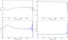Fig. 3 Upper panel: example of kernel fits for the inversion of the acoustic radius of 16CygA (averaging kernel on the left and cross-term kernel on the right). Lower panel: kernel fits for the inversion of the mean density for 16CygA (averaging kernel on the left and cross-term kernel on the right). The target functions are in green and the SOLA kernels in blue.

2.3. Determination of new reference models

After having carried out a first set of inversions using the acoustic radius and the mean density, we carried out a supplementary step of model parameter determination, replacing the average large frequency separation by the acoustic radius and the mean density themselves. We obtained a new family of reference models that were slightly different from those obtained using the average large frequency separation. We used the following naming convention for these models: the first letter, A or B is associated with the star, namely 16CygA or 16CygB; the second letter is associated with the chemical composition box in the right-hand panel of Fig. 7, where C is the central chemical composition, L the left-hand side, R the right-hand side, U the upper side, and D the lower side (D for down); the number 1 or 2 is associated with diffusion, 1 for models without microscopic diffusion, and 2 for models including the prescriptions of Thoul et al. (1994) for microscopic diffusion. The numerical results of these supplementary fits are given in Table A.1 for the A component and in Table A.2 for the B component. A summary of the two steps of forward modelling and the naming conventions associated to the models can be found in Table 4.

If we compare the model parameters obtained using τ and for the model with Y_f = 0.24 and (Z/X)_f = 0.0222 (following our naming convention, model S_A,C,1) with those obtained with ⟨ Δν ⟩, presented in Table 2 for model S_A,1, we note that there is a tendency to reduce the mass slightly and to increase the mixing length parameter. The same tendency is observed for the corresponding models including microscopic diffusion. What is more surprising is that when computing individual frequency differences between the observed stars and the reference models, we see that using the acoustic radius and the mean density allows us to obtain significantly better individual frequencies. This is a by-product of the use of inversion techniques that could be used to characterise stars in a pipeline such as what will be developed for the upcoming PLATO mission (Rauer et al. 2014).

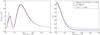Fig. 4 Left panel: effect of diffusion, metallicity changes and helium abundance changes on the core regions for models SA,C1, SA,C2, SA,L1, SA,U1 on the target function of tu. Since the quantity is integrated, the sensitivity is greatly improved. Right panel: the Y(x) profile of these models is illustrated, thus showing the link between tu and chemical composition and thus, its diagnostic potential.

Considering that these models are improved compared to what was obtained using the large frequency separation³, we computed a family of models for different values of Y_f and ${{}^{\mathrm{\right(}}\frac{\mathit{Z}}{\mathit{X}}^{\mathrm{\left)}}}_{\mathit{f}}$. For each particular chemical composition, we computed models with and without microscopic diffusion. The properties of some models of this family are summarised in Table A.1. As can be seen, some of the models do not reproduce the results for the effective temperature or the interferometric radius well. This means that we can use non-seismic constraint as indicators of inconsistent models in our study, although one should be careful about the conclusions derived from these quantities. For instance, the interferometric radii are different from the radii computed with the Clés models and some differences might result from the very definition of the radius. One should also note that these results are not totally incompatible since White et al. (2013) conclude that the radius of 16CygA is 1.22 ± 0.02 R_⊙ and we find values around 1.185 and 1.230, outside the 1σ errors for the lower part of our scatter. The stellar luminosity also depends on these radii values and so should be considered with care. Ultimately, the effective temperature can be constraining although there might be a slight difference stemming from discrepancies between the physical ingredients in the stellar atmosphere models used for the spectroscopic study of Ramírez et al. (2009) and Tucci Maia et al. (2014) and those used in the Clés models in this paper. However, the inconsistencies observed for some of these models are too important and therefore these models should be rejected. The combination of all the information available are described in Sect. 4. In the next section, we use these models as references for our inversions of the t_u indicator. One should note that this first step was beneficial since obtaining reference models as accurate as possible for these stars is the best way to obtain accurate results for the more difficult inversion of the t_u indicator.

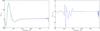Fig. 5 Example of kernel fits for the tu inversion. The left panel is associated with the averaging kernel and the right panel is associated with the cross-term kernel. The target functions are in green and the SOLA kernels in blue.

3. Inversion results for the t_u core condition indicator

3.1. Definition of the indicator and link to mixing processes

In Buldgen et al. (2015a), we defined and tested a new indicator for core conditions, which is applicable to a large number of stars⁴ and very sensitive to microscopic diffusion or chemical composition mismatches in the core regions between the target and the reference model. The definition of this quantity was the following: 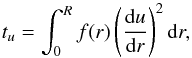$\begin{array}{ccc}{\mathit{t}}_{\mathit{u}}\mathrm{=}{\mathrm{\int }}_{\mathrm{0}}^{\mathit{R}}\mathit{f}\mathrm{\left(}\mathit{r}\mathrm{\right)}{\left(\frac{\mathrm{d}\mathit{u}}{\mathrm{d}\mathit{r}}\right)}^{\mathrm{2}}\mathrm{d}\mathit{r,}& & \end{array}$(3)where u is the squared isothermal sound speed, defined as $\mathit{u}\mathrm{=}\frac{\mathit{P}}{\mathit{\rho }}$, f(r) is a weighting function defined as follows: 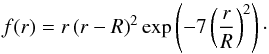$\begin{array}{ccc}\mathit{f}\mathrm{\left(}\mathit{r}\mathrm{\right)}\mathrm{=}\mathit{r}{\mathrm{(}\mathit{r}\mathrm{-}{\mathit{R}}^{\mathrm{)}}}^{\mathrm{2}}\exp \left(\mathrm{-}\mathrm{7}{\left(\frac{\mathit{r}}{\mathit{R}}\right)}^{\mathrm{2}}\right)\mathrm{·}& & \end{array}$(4)Owing to the effects of the radius differences between the observed target and reference model, we noted that the quantity measured was $\frac{{\mathit{t}}_{\mathit{u}}}{{\mathit{R}}_{\mathrm{tar}}^{\mathrm{6}}}$, where R_tar is the target radius. In Fig. 4, we illustrate the changes in the quantity from the effects of diffusion for two of our reference models, having the same surface chemical composition and fitting the same observational constraints. One can also see the effects of surface helium and metallicity changes on the profile of the integrant of Eq. (3). The whole parameter set of these models is given in Table A.1 along with the explanation of the naming convention. The diagnostic potential of the t_u inversion is therefore clear, although the weighting function could be adapted to suit other needs if necessary. The inversion of this integrated quantity can be made using both the ${}^{\mathrm{(}}\mathit{u}_{\mathrm{0}}\mathit{,}{\mathrm{\Gamma }}_{\mathrm{1}}{\mathrm{)}}^{}$ or the ${}^{\mathrm{(}}\mathit{u}_{\mathrm{0}}\mathit{,}{\mathit{Y}}^{\mathrm{)}}$ kernels.

3.2. The SOLA inversion technique

To carry out inversions of integrated quantities, we use the SOLA linear inversion technique developed by Pijpers & Thompson (1994). This technique uses the linear combinations of individual frequency differences to induce structural corrections. It is commonly used in helioseismology and has been recently adapted to the inversion of integrated quantities for asteroseismic targets. The philosophy of the SOLA inversion technique is to use a kernel-matching approach to derive the structural corrections. For the particular example of the t_u inversion, one would be using the following cost function: $\begin{array}{ccc}{\mathrm{𝒥}}_{{\mathit{t}}_{\mathit{u}}}& \mathrm{=}& \int \begin{array}{c}\mathrm{1}\\ \mathrm{0}\end{array}{\mathrm{[}{\mathit{K}}_{\mathrm{Avg}}\mathrm{-}{\mathrm{𝒯}}_{{\mathit{t}}_{\mathit{u}}}\mathrm{]}}^{\mathrm{2}}\mathrm{d}\mathit{x}\mathrm{+}\mathit{\beta }{\mathrm{\int }}_{\mathrm{0}}^{\mathrm{1}}{\mathit{K}}_{\mathrm{Cross}}^{\mathrm{2}}\mathrm{d}\mathit{x}\mathrm{+}\tan \mathrm{\left(}\mathit{\theta }\mathrm{\right)}\sum _{\mathit{i}}^{\mathit{N}}\mathrm{(}{\mathit{c}}_{\mathit{i}}{\mathit{\sigma }}_{\mathit{i}}{\mathrm{)}}^{\mathrm{2}}\\ & & \mathrm{+}\mathit{\eta }\left[\sum _{\mathit{i}}^{\mathit{N}}{\mathit{c}}_{\mathit{i}}\mathrm{-}\mathit{k}\right]\mathit{,}\end{array}$(5)where K_Avg is the so-called averaging kernel and K_Cross the so-called cross-term kernel defined as follows for the (u,Y) structural pair: $\begin{array}{ccc}{\mathit{K}}_{\mathrm{Avg}}\mathrm{=}\sum _{\mathit{i}}^{\mathit{N}}{\mathit{c}}_{\mathit{i}}{\mathit{K}}_{\mathit{u,Y}}^{\mathit{i}}\mathit{,}& & \\ {\mathit{K}}_{\mathrm{Cross}}\mathrm{=}\sum _{\mathit{i}}^{\mathit{N}}{\mathit{c}}_{\mathit{i}}{\mathit{K}}_{\mathit{Y,u}}^{\mathit{i}}\mathit{.}& & \end{array}$The symbols θ and β are free parameters of the inversion and thus can change for a given indicator or observed frequency sets. Here, θ is related to the compromise between reducing the observational error bars (σ_i) and improving the averaging kernel, whereas β is allowed to vary to give more weight to elimination of the cross-term kernel. One should note that, ultimately, adjusting these free parameters is a problem of compromise and is made through hare-and-hounds exercises that have been presented in our previous papers. Various sanity checks can be used to analyse the robustness of the results. For example, one can use various reference models and analyse the variability of the inversion results or one can also use different structural pairs and see if this effect changes the results significantly.

In this expression of the kernels, N is the number of observed frequencies, c_i are the inversion coefficients, used to determine the correction that will be applied on the t_u value, η is a Lagrange multiplier and the last term appearing in the expression of the cost-function is a supplementary constraint applied to the inversion. Ultimately the correction on the t_u value obtained by the inversion is 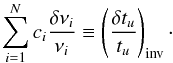$\begin{array}{ccc}\sum _{\mathit{i}\mathrm{=}\mathrm{1}}^{\mathit{N}}{\mathit{c}}_{\mathit{i}}\frac{\mathit{\delta }{\mathit{\nu }}_{\mathit{i}}}{{\mathit{\nu }}_{\mathit{i}}}\mathrm{\equiv }{\left(\frac{\mathit{\delta }{\mathit{t}}_{\mathit{u}}}{{\mathit{t}}_{\mathit{u}}}\right)}_{\mathrm{inv}}\mathrm{·}& & \end{array}$(8)One should note that the value obtained is an estimate whereas the previous equality is a definition. In fact, the inversion depends on some hypotheses that are used throughout the mathematical developments of the relation between frequency differences and structural differences and the definition of t_u. One should note that the particular definition of the cost function given above is very similar to the general expression for any integrated quantity and local correction, since one only has to change the target function, here denoted , to obtain other corrections.

3.3. Inversion results for 16CygA

The inversion results are summarised in Fig. 7 (represented as orange × in the $\mathit{\rho ̅}\mathrm{-}\frac{{\mathit{t}}_{\mathit{u}}}{{\mathit{R}}^{\mathrm{6}}}$ plot) and illustrated through an example of kernel fits in Fig. 5. We tried using both the ${}^{\mathrm{(}}\mathit{u}_{\mathrm{0}}\mathit{,}{\mathrm{\Gamma }}_{\mathrm{1}}{\mathrm{)}}^{}$ and the ${}^{\mathrm{(}}\mathit{u}_{\mathrm{0}}\mathit{,}{\mathit{Y}}^{\mathrm{)}}$ kernels. The high amplitude of the Γ₁ cross-term leads us to present the results from the ${}^{\mathrm{(}}\mathit{u}_{\mathrm{0}}\mathit{,}{\mathit{Y}}^{\mathrm{)}}$ kernels instead although they are quite similar in terms of the inverted values. However, one should note that the error bars are quite important, and we have to be careful when interpreting the inversion results.

This effect is due to both the very high amplitude of the inversion coefficients and the amplitude of the observational error bars. When compared to the somewhat underestimated error bars of the acoustic radius and mean density inversion, it illustrates perfectly well why it is always said that two inversion problems can be completely different. In this particular case, using various reference models allows us to already see a trend in the inversion results. We clearly see that the value of t_u for our reference models is too low and that the scatter of the inversion results is rather low, despite the large error bars. One should also note that the quality of the kernel fit is also a good indicator of the quality of the inverted result. For most cases, the kernels were very well fitted and the low scatter of the results means that there is indeed information to be extracted from the inversion. We will see how this behaviour is different for 16CygB.

Nevertheless, one could argue that a small change in t_u could be easily obtained through the use of diffusion or chemical composition changes. We see in Sect. 4 how combining all the information with new constraints from the inversion technique can be extremely restrictive in terms of chemical composition and diffusion processes. Indeed, t_u should not be considered as a model-independent age determination or as an observed quantity that disentangles all physical processes occurring in stellar cores. In fact, it is simply a nearly model-independent determination of a structural quantity optimised to be more sensitive to any change in the physical conditions in stellar cores than classical seismic indicators. The amplitude of the error bars reminds us that this sensitivity comes at a cost and in this study we consider that having a reference model with a $\frac{{\mathit{t}}_{\mathit{u}}}{{\mathit{R}}_{\mathrm{ref}}^{\mathrm{6}}}\mathrm{\approx }\mathrm{3.2}$ or 3.3$\frac{{\mathrm{g}}^{\mathrm{2}}}{{\mathrm{cm}}^{\mathrm{6}}}$ will be acceptable if it still fits the other observational constraints.

3.4. Inversion results for 16CygB

The case of 16CygB is completely different. In fact, while the inversion for the acoustic radius and the mean density have been successful and we could build improved models for this star, the inversion of the t_u indicator was less successful. The results were good, in the sense that the kernels are well fitted. However, we can see from Fig. 6 that the amplification of the observational errors was too high to constrain the microscopic diffusion effects or the chemical composition. In fact, it is not surprising since the error bars on the observed frequencies are larger than for 16CygA.

As a matter of fact, the observational errors dominate the inversion result, as can be easily shown in Fig. 6. We see that the relative change in t_u is smaller when microscopic diffusion is included in the model but this is because the inversion result is closer to the reference value rather than the opposite. This therefore means that t_u can be used as a consistency check for future investigations to ensure that we stay within the error bars of the inverted value, but it seems that we cannot gain additional information for this star from this indicator.

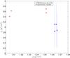Fig. 6 tu inversion results for 16CygB. The red + are the reference models and the blue × the inverted results. The lower + are associated with the upper × and refer to models including solar-calibrated diffusion.

4. Constraints on microscopic diffusion and chemical composition

4.1. Reducing the age, mass and radius scatter of 16CygA

In this section, we use the information given by t_u to further constrain chemical composition and microscopic diffusion. Previously, we always ensured that the reference models were inside the chemical composition box that was defined by the constraints on surface helium obtained by Verma et al. (2014) and the spectroscopic constraints on surface metallicity obtained by Ramírez et al. (2009). In Sect. 3.3, we concluded that our model should have at least a $\frac{{\mathit{t}}_{\mathit{u}}}{{\mathit{R}}_{\mathrm{ref}}^{\mathrm{6}}}\mathrm{\approx }\mathrm{3.2}$ or 3.3$\frac{{\mathrm{g}}^{\mathrm{2}}}{{\mathrm{cm}}^{\mathrm{6}}}$ or higher. The first question that arises is whether it is possible to obtain such values for $\frac{{\mathit{t}}_{\mathit{u}}}{{\mathit{R}}^{\mathrm{6}}}$ given the constraints on chemical composition. The second question is related to the impact of microscopic diffusion.

In fact, t_u is a measure of the intensity of the squared isothermal sound speed, u₀, gradients in the core regions. Thus, since ${\mathit{u}}_{\mathrm{0}}\mathrm{\approx }\frac{\mathit{T}}{\mathit{\mu }}$, where T is the temperature and μ the mean molecular weight, including diffusion will increase the μ gradients, since it leads to the separation of heavy elements from lighter elements. It is then possible to increase the diffusion speed of the chemical elements significantly and to obtain a very high value of t_u for nearly any chemical composition. However, in Thoul et al. (1994), the diffusion speed is said to be accurate to within ~15−20% and suited to solar conditions. Moreover, since increasing diffusion also accelerates the evolution, we could also end up with models that are too evolved to simultaneously fit t_u, the chemical composition constraints and the seismic constraints. Looking at the parameters of our reference models, we note that we are indeed very close to solar conditions, and we suppose that our diffusion speed should not be amplified or damped by more than 20%. The results of this analysis are summarised in Fig. 7, which is a $\mathit{\rho ̅}\mathrm{-}\frac{{\mathit{t}}_{\mathit{u}}}{{\mathit{R}}^{\mathrm{6}}}$ plot where the reference models and the inverted results are represented. In what follows, we describe our reasoning more precisely and refer to Fig. 7 when necessary. We used a particular colour code and type of symbol to describe the changes we applied to our models. One should keep in mind that these models are still built using the Levenberg-Marquardt algorithm and thus still fit the constraints used previously in the cost function. Firstly, colour is associated with the final surface helium mass fraction Y_f: blue for Y_f = 0.24, red if Y_f< 0.24, and green if Y_f> 0.24. Secondly, the symbol itself is related to the ${{}^{\mathrm{\right(}}\frac{\mathit{Z}}{\mathit{X}}^{\mathrm{\left)}}}_{\mathit{f}}$: a × for ${{}^{\mathrm{\right(}}\frac{\mathit{Z}}{\mathit{X}}^{\mathrm{\left)}}}_{\mathit{f}}\mathit{<}\mathrm{0.0222}$, a ° for ${{}^{\mathrm{\right(}}\frac{\mathit{Z}}{\mathit{X}}^{\mathrm{\left)}}}_{\mathit{f}}\mathrm{=}\mathrm{0.0222}$, and a ⋄ for ${{}^{\mathrm{\right(}}\frac{\mathit{Z}}{\mathit{X}}^{\mathrm{\left)}}}_{\mathit{f}}\mathit{>}\mathrm{0.0222}$. The size of the symbol is related to the inclusion of microscopic diffusion, for example the large blue and red circles in Fig. 7 are related to models that include microscopic diffusion.

Since increasing diffusion should increase the t_u value, we computed a model with Y_f = 0.24 and ${{}^{\mathrm{\right(}}\frac{\mathit{Z}}{\mathit{X}}^{\mathrm{\left)}}}_{\mathit{f}}\mathrm{=}\mathrm{0.0222}$, including diffusion from Thoul et al. (1994) and fitting the seismic constraints and the effective temperature. This model is represented by the large blue dot and we note that including diffusion improves the agreement, but is not sufficient to reach what we defined to be our acceptable values for $\frac{{\mathit{t}}_{\mathit{u}}}{{\mathit{R}}^{\mathrm{6}}}$. This is illustrated by the fact that in Fig. 7, the large blue circle is above the small blue dot. Therefore we decided to analyse how t_u depends on the chemical composition. To do so, we computed a model for each corner and each side of the chemical composition box. These models are represented in Fig. 7 by the ⋄, °, and × of various colours. From these results, we see that increasing the helium content, namely considering that Y_f ∈ [0.24,0.25] increases t_u, as does considering ${{}^{\mathrm{\right(}}\frac{\mathit{Z}}{\mathit{X}}^{\mathrm{\left)}}}_{\mathit{f}}\mathrm{\in }\left[\mathrm{0.0209}\mathit{,}\mathrm{0.0222}\right]$. In simpler terms, we see that the green circle and the blue circle are above the blue dot in Fig. 7.

Fig. 7 Results of the tu inversions for 16CygA (left panel) and positions of the reference models in the chemical composition box derived from spectroscopic and seismic constraints (right panel). The orange × are the inversion results whereas the other symbols are associated with various reference models the positions of which are shown in the right-hand plot. The colour is associated with the Yf value, the type of symbol with the ${{}^{\mathrm{\right(}}\frac{\mathit{Z}}{\mathit{X}}^{\mathrm{\left)}}}_{\mathit{f}}$ value, and the size of the symbol with the inclusion of diffusion.

The first tendency is quickly understood since increasing the helium abundance leads to higher central μ and therefore a local minimum in the u₀ profile. Because t_u is based on ${{}^{\mathrm{\right(}}\frac{\mathrm{d}\mathit{u}}{\mathrm{d}\mathit{x}}^{\mathrm{\left)}}}^{\mathrm{2}}$, this does not imply a reduction in the value of the indicator, but an increase due to a secondary lobe developing exactly in the same way as what happens when including diffusion (see Fig. 2). The second tendency can be understood by looking at the central hydrogen abundance. In this case, we see that the central hydrogen abundance is reduced and thus the mean molecular weight is increased and leads to a minimum in u₀ in the centre. One should note that this effect is not as intense as the change in helium but is still non-negligible.

Therefore, our seismic analysis favours models that lie within Y_f ∈ [0.24,0.25] and ${{}^{\mathrm{\right(}}\frac{\mathit{Z}}{\mathit{X}}^{\mathrm{\left)}}}_{\mathit{f}}\mathrm{\in }\left[\mathrm{0.0209}\mathit{,}\mathrm{0.0222}\right]$. Including diffusion in these models increases the $\frac{{\mathit{t}}_{\mathit{u}}}{{\mathit{R}}^{\mathrm{6}}}$ value even more and brings it in the range of the 3.2, 3.3$\frac{{\mathrm{g}}^{\mathrm{2}}}{{\mathrm{cm}}^{\mathrm{6}}}$ values, which is much more consistent with the inversion results. These final models are represented in Fig. 7 by the large green +. One should also note that an upper boundary can be drawn from the effective temperature, interferometric radius and the seismic constraints. In other words, the fit of the other quantities can increase slightly up to values of 1.6 and thus slightly reduce the quality of the fit. This is not alarming but still means that one should not put all the weight of the fit of the model on the inversion results but try to find a compromise between seismic, spectroscopic, and inverted constraints. Looking at Fig. 7, we can also see that the models do not fit the mean density values. This is due to improper fitting in the Levenberg-Marquardt algorithm. In fact, to build Fig. 7, we put more weight on the surface chemical composition, the acoustic radius and the seismic constraints at the expense of the mean density. This does not change the results on the t_u inversion since the vertical trend can also be seen for a model fitting the mean density value used in Fig. 7. It is also noteworthy to mention that the mean density values obtained for the models presented in Fig. 7 correspond to the value obtained without the polynomial surface correction. As we stated before, only further investigations with models including strong surface effects will be able to distinguish which of both values for the mean density inversions should be used.

Ultimately, when considering models built with the Levenberg-Marquardt algorithm that are compatible with the t_u values, we are able to reduce the scatter previously observed. We thus conclude that the mass of 16CygA must be between 0.96 M_⊙ and 1.0 M_⊙, and its age must be between 7.0Gy and 7.4Gy. These values are subject to the hypotheses of this study and they depend on the physics used in the stellar models (opacities, nuclear reaction rates, abundances). We recall here that there is no way to provide a seismic fully model-independent age, but inversions allow us to at least check the consistency of our models with less model-dependent structural quantities. These consistency checks can lead to a refinement of the model parameters and, in this particular case, to constraints on microscopic diffusion.

For the sake of completion, we also analysed the importance of the abundances used to build the model. Because the [Fe/H] constraint are extremely dependent on the solar ${{}^{\mathrm{\right(}}\frac{\mathit{Z}}{\mathit{X}}^{\mathrm{\left)}}}_{\mathrm{\odot }}$, we wanted to ask the question of whether the inversion would have also provided a diagnostic if we had used the GN93 abundances to determine the metallicity. Using these abundances and the associated ${{}^{\mathrm{\right(}}\frac{\mathit{Z}}{\mathit{X}}^{\mathrm{\left)}}}_{\mathrm{\odot }}$ which is equal to 0.0244, one ends up with models having much higher metallicities, of the order of 0.0305 when no diffusion is included in the model. In fact we ended up with the same tendencies in the chemical composition box, but with completely different values of ${}^{\mathrm{\right(}}\frac{\mathit{Z}}{\mathit{X}}^{\mathrm{\left)}}$, implying slightly higher masses of around 1.03 M_⊙ and slightly lower ages around 6.8 Gy. However, when carrying out the t_u inversion, we noted that we still had to increase the helium content, include diffusion, and reduce the ${}^{\mathrm{\right(}}\frac{\mathit{Z}}{\mathit{X}}^{\mathrm{\left)}}$. The interesting point was that even the lowest ${}^{\mathrm{\right(}}\frac{\mathit{Z}}{\mathit{X}}^{\mathrm{\left)}}$, associated with the highest Y_f with increased diffusion could not produce a sufficiently high value of t_u. In that sense, it tends to prove what we already suspected, that the GN93 abundances should not be used in the spectroscopic determination of the ${}^{\mathrm{\right(}}\frac{\mathit{Z}}{\mathit{X}}^{\mathrm{\left)}}$ for this study. In this particular case, we see that the inversion of t_u is able to detect such inconsistencies, thanks to its sensitivity to metallicity mismatches. However, if the model is built with the ${}^{\mathrm{\right(}}\frac{\mathit{Z}}{\mathit{X}}^{\mathrm{\left)}}$ determined from the AGSS09 solar reference value, but using the GN93 solar heavy element mixture, we cannot detect inconsistencies. In fact, we obtain the same conclusion as before since these models are nearly identical in terms of internal structure.

4.2. Impact on the mass and radius scatter of 16CygB

In the previous section, we used the t_u inversion to reduce the age, mass and radius scatter of 16CygA. Moreover, we know from Sect. 3.4 that the inversion of t_u for 16CygB can only be used to check the consistency of the model but not to gain additional information. However, since these stars are binaries, we can say that the age values of the models 16CygB must be compatible with those obtained for 16CygA. From the inversion results of 16CygA, we have also deduced that we had to include atomic diffusion in the stellar models and since both stars are very much alike, there is no reason to discard microscopic diffusion from the models of the B component when we know that it has to be included in the models for the A component.

Therefore, we can ask the question of what would the mass and radius of 16CygB be if one includes diffusion as in 16CygA and ensures that the ages of the models remain compatible. The question of the chemical composition is also important since Ramírez et al. (2009) find a somewhat lower value for the [Fe/H] of the B component and Verma et al. (2014) found larger uncertainties for the surface helium abundance, although the centroid value was the same as that of 16CygA.

To build these new models, we imposed that they include atomic diffusion with a coefficient D of 1.0 or 1.15. The age was to be between 7.0 Gy and 7.4 Gy. The metallicity was required to be within the error bars provided by Ramírez et al. (2009) and the surface helium abundance was to be within [0.24,0.25]. We used the same constraints as before to carry out the fits using the Levenberg-Marquardt algorithm and found that the mass was to be within 0.93 M_⊙ and 0.96 M_⊙, thus a 1.5% uncertainty and the radius was to be within 1.08 R_⊙ and 1.10 R_⊙, hence a 1% uncertainty. We would like to emphasize here that these values do of course depend on the results of the modelling of 16CygA and are thus more model-dependent since they do not result from constraints obtained through seismic inversions. They are a consequence of the binarity of the system. It is clear that a change in the values of the fundamental parameters for 16CygA will induce a change in the values of 16CygB.

4.3. Discussion

The starting point of this study was to determine fundamental parameters for both 16CygA and 16CygB using seismic, spectroscopic, and interferometric constraints. However, the differences between our results and those from Metcalfe et al. (2012) raise questions. One could argue that the inversion leads to problematic results and that the diagnostic would have been different if the surface helium determination from Verma et al. (2014) would have not been available.

Therefore, for the sake of comparison, we asked the question of what would have been the results of this study if we had not included the surface helium abundance from Verma et al. (2014) in the model-selection process. We carried out a few supplementary fits, using the mass, age, α_MLT, X₀ and Z₀ as free parameters, using all the previous observational constraints as well as the prescription for microscopic diffusion from Thoul et al. (1994), but excluding the Y_f value. The results speak for themselves since we end up with a model for the A component having a mass of 1.09 M_⊙ and an age of 7.19Gy compatible with the results from Metcalfe et al. (2012). This means that the determining property that leads to the changes in the fundamental parameters of the star was, as previously guessed, the surface helium value. Without this Y_f constraint, therefore, one would end up with two solutions with completely different masses and ages, but solutions that fit the same observational constraints. This does not mean that the results from Metcalfe et al. (2012) are wrong, but that they were simply the best results one could obtain without the surface helium constraint and with three months of Kepler data. In fact, this is only an illustration of the importance of chemical composition constraints in stellar physics. The Y₀ − M trend has already been described in Baudin et al. (2012) and that we find lower masses when increasing the helium abundance is, ultimately, no surprise.

At this point, we wanted to know what the inversion results would have been if we had used reference models with similar parameters as obtained in Metcalfe et al. (2012). We ended up with similar results for both the acoustic radius and the mean density inversion, but more interestingly, the t_u inversion also provided non-negligible corrections for this model. In fact, even with microscopic diffusion, the $\frac{{\mathit{t}}_{\mathit{u,}\mathrm{ref}}}{{\mathit{R}}_{\mathrm{Ref}}^{\mathrm{6}}}$ value was: 2.72 g²/ cm⁶ whereas the inverted result was $\frac{{\mathit{t}}_{\mathit{u,}\mathrm{inv}}}{{\mathit{R}}_{\mathrm{obs}}^{\mathrm{6}}}\mathrm{=}\mathrm{3.5}\mathrm{\pm }\mathrm{0.5}{\mathrm{g}}^{\mathrm{2}}\mathit{/}{\mathrm{cm}}^{\mathrm{6}}$. Therefore the diagnostic potential of the indicator is still clear, since it could have provided indications for a change in the core structure of the model. Assuming that diffusion velocities are accurate to around 20%, one could have invoked either an extra-mixing process or a change in the initial helium composition to explain this result. Disentangling both cases would then have probably required additional indicators.

5. Conclusion

In this article, we have applied the inversion techniques presented in a series of previous papers to the binary system 16CygA and 16CygB. The first part of this study consisted in determining suitable reference models for our inversion techniques. This was done using a Levenberg-Marquardt algorithm and all the seismic, spectroscopic and interferometric observational constraints available. We used the oscillation frequencies from Davies et al. (2015), the interferometric radii from White et al. (2013), the spectroscopic constraints from Ramírez et al. (2009) and Tucci Maia et al. (2014), and the surface helium constraints from Verma et al. (2014).

These constraints on the surface chemical composition mean that our results are different from those of Metcalfe et al. (2012). The test case we made without using the constraint on surface helium from Verma et al. (2014) demonstrates the importance of constraints on the chemical composition for seismic studies. In fact, having to change the initial helium abundance from 0.25 to values around 0.30 is of course not negligible. This emphasizes that we have to be careful when using free parameters for the stellar chemical composition in seismic modelling. The same can be said for the constraints on the stellar [Fe/H] from the study of Ramírez et al. (2009). For this particular constraint, we have to add the importance of the solar mixture used in the spectroscopic study. Owing to the important changes in the ${{}^{\mathrm{\right(}}\frac{\mathit{Z}}{\mathit{X}}^{\mathrm{\left)}}}_{\mathrm{\odot }}$ from the GN93 abundances to the AGSS09 abundances, we tested both abundances and found that the latter produces better results. We note that our reference models tend to be consistent with the spectroscopic, seismic and interferometric constraints and that independent modelling of both stars leads to consistent ages. We also note the presence of a certain modelling degeneracy in terms of chemical composition and microscopic diffusion. Accordingly, we could obtain rather different values for the mass, the radius and the age of both stars by assuming more intense diffusion and changing the chemical composition within the error bars from both Ramírez et al. (2009) and Verma et al. (2014).

Having obtained suitable reference models, we then carried out inversions for the mean density , the acoustic radius τ, and a core condition indicator t_u. The first two quantities were used to improve the quality of the reference models. As a by-product, we noted that models fitting both and τ were in better agreement in terms of individual frequencies. We also found that both of these quantities could not differentiate the effect of the degeneracy in terms of diffusion and chemical composition. However, they could be well suited to analysing uppers layers along with other quantities.

After the second modelling process, we carried out inversion for the t_u indicator and noted that the degeneracy in terms of chemical composition and diffusion could be lifted for 16CygA. In fact, to agree with the inverted result, one has to consider the same diffusion speed as used in Thoul et al. (1994) for the solar case or slightly higher (by 10% or 15%). Values higher than 20% were considered not to be physical by Thoul et al. (1994) and were therefore not analysed in this study. Ultimately, we come up with a lower scatter in terms of mass and age for 16CygA, namely that this component should have a mass between 0.97 M_⊙ and 1.0 M_⊙, a radius between 1.188 R_⊙ and 1.200 R_⊙ and an age between 7.0 Gy and 7.4 Gy. Again the slight differences between the seismic radius provided here and the interferometric radius might stem from different definitions of the interferometric radius and the seismic one. We also conclude that the t_u inversion for 16CygB could only be used as a consistency check but could not help reduce the scatter in age. However, as these stars are binaries, a reduced age scatter for one component means that the second has to be consistent with this smaller age interval. Therefore, we were able to deduce a smaller mass and radius scatter for the second component, namely between 0.93 M_⊙ and 0.96 M_⊙ and between 1.08 R_⊙ and 1.10 R_⊙. We also note that when not considering the constraints on surface helium, we obtained results compatible with Metcalfe et al. (2012) but the t_u values were too low even when diffusion was included in the models. This reinforces the importance of constraints on the chemical composition and illustrates to what extent inversions could be used given their intrinsic limitations.

Finally, we draw the attention of the reader to the following points. The age values we obtain are not model-independent, because we assumed physical properties for the models and assumed that the agreement in t_u was to be improved by varying the chemical composition within the observational constraints and by calibrating microscopic diffusion. This does not mean that no other mixing process has taken place during the evolutionary sequence that could somehow bias our age determination slightly. In that sense, further improved studies will be carried out, using additional structural quantities, more efficient global minimization tools for the selection of the reference models, and possibly improved physical ingredients for the models. In conclusion, we show in this study that inversions are indeed capable of improving our use of seismic information and therefore, through synergies with stellar modellers, of helping us build new generations of more physically accurate stellar models.

Acknowledgments

G.B. is supported by the FNRS (“Fonds National de la Recherche Scientifique”) through a FRIA (“Fonds pour la Formation à la Recherche dans l’Industrie et l’Agriculture”) doctoral fellowship. D.R.R. is currently funded by the European Community’s Seventh Framework Programme (FP7/2007–2013) under grant agreement No. 312844 (SPACEINN), which is gratefully acknowledged. This article made use of an adapted version of InversionKit, a software developed in the context of the HELAS and SPACEINN networks, funded by the European Commissions’s Sixth and Seventh Framework Programmes. We would also like to thank Guy Davies for his advice.

References

Appendix A: Intermediate results of the forward modelling process

After the first step of forward modelling, we carried out supplementary fits to obtain new reference models for both 16CygA and 16CygB. In fact, we replaced the average large frequency separation by the acoustic radius and the mean density, as discussed in Sect. 2.3. We recall here the naming convention for these models: the first letter, A or B is associated with the star, namely 16CygA or 16CygB; the second letter is associated with the chemical composition box in the right panel of Fig. 7: C is the central chemical composition, L the left-hand side, R the right-hand side, U the upper side, and D the lower side (D for down); the number 1 or 2 is associated with diffusion, 1 is for models without microscopic diffusion, 2 is for models including the prescriptions of Thoul et al. (1994) for microscopic diffusion. These results are illustrated in the Tables A.1 and A.2 for both stars.

All Tables

All Figures

Fig. 1 Upper panel: fits of the small frequency separations $\begin{array}{c}{\mathrm{˜}}_{}\\ {\mathit{\delta }}_{\mathrm{02}}\end{array}$ and $\begin{array}{c}{\mathrm{˜}}_{}\\ {\mathit{\delta }}_{\mathrm{13}}\end{array}$ for 16CygA. Lower panel: same as the upper panel for 16CygB. The observational values are the green symbols with error bars, the red symbols are associated with models including solar-calibrated diffusion and the blue symbols are associated with models without diffusion.

In the text

	Fig. 2 Effect of the progressive inclusion of diffusion in a model of 16CygA. Each model still fits the observational constraints.
In the text

	Fig. 3 Upper panel: example of kernel fits for the inversion of the acoustic radius of 16CygA (averaging kernel on the left and cross-term kernel on the right). Lower panel: kernel fits for the inversion of the mean density for 16CygA (averaging kernel on the left and cross-term kernel on the right). The target functions are in green and the SOLA kernels in blue.
In the text

Fig. 4 Left panel: effect of diffusion, metallicity changes and helium abundance changes on the core regions for models SA,C1, SA,C2, SA,L1, SA,U1 on the target function of tu. Since the quantity is integrated, the sensitivity is greatly improved. Right panel: the Y(x) profile of these models is illustrated, thus showing the link between tu and chemical composition and thus, its diagnostic potential.

In the text

	Fig. 5 Example of kernel fits for the tu inversion. The left panel is associated with the averaging kernel and the right panel is associated with the cross-term kernel. The target functions are in green and the SOLA kernels in blue.
In the text

	Fig. 6 tu inversion results for 16CygB. The red + are the reference models and the blue × the inverted results. The lower + are associated with the upper × and refer to models including solar-calibrated diffusion.
In the text

Fig. 7 Results of the tu inversions for 16CygA (left panel) and positions of the reference models in the chemical composition box derived from spectroscopic and seismic constraints (right panel). The orange × are the inversion results whereas the other symbols are associated with various reference models the positions of which are shown in the right-hand plot. The colour is associated with the Yf value, the type of symbol with the ${{}^{\mathrm{\right(}}\frac{\mathit{Z}}{\mathit{X}}^{\mathrm{\left)}}}_{\mathit{f}}$ value, and the size of the symbol with the inclusion of diffusion.

In the text

References

- Angulo, C., Arnould, M., Rayet, M., et al. 1999, Nucl. Phys. A, 656, 3 [NASA ADS] [CrossRef] [Google Scholar]
- Asplund, M., Grevesse, N., Sauval, A. J., & Scott, P. 2009, ARA&A, 47, 481 [NASA ADS] [CrossRef] [Google Scholar]
- Basu, S., & Christensen-Dalsgaard, J. 1997, A&A, 322, L5 [NASA ADS] [Google Scholar]
- Basu, S., Christensen-Dalsgaard, J., Schou, J., Thompson, M. J., & Tomczyk, S. 1996, Bull. Astron. Soc. India, 24, 147 [NASA ADS] [Google Scholar]
- Basu, S., Christensen-Dalsgaard, J., Chaplin, W. J., et al. 1997, MNRAS, 292, 243 [NASA ADS] [CrossRef] [Google Scholar]
- Baudin, F., Barban, C., Goupil, M. J., et al. 2012, A&A, 538, A73 [NASA ADS] [CrossRef] [EDP Sciences] [Google Scholar]
- Böhm-Vitense, E. 1958, Z. Astrophys., 46, 108 [Google Scholar]
- Buldgen, G., Reese, D. R., & Dupret, M. A. 2015a, A&A, 583, A62 [NASA ADS] [CrossRef] [EDP Sciences] [Google Scholar]
- Buldgen, G., Reese, D. R., Dupret, M. A., & Samadi, R. 2015b, A&A, 574, A42 [NASA ADS] [CrossRef] [EDP Sciences] [Google Scholar]
- Cassisi, S., Potekhin, A. Y., Pietrinferni, A., Catelan, M., & Salaris, M. 2007, ApJ, 661, 1094 [NASA ADS] [CrossRef] [Google Scholar]
- Christensen-Dalsgaard, J. 2002, Rev. Mod. Phys., 74, 1073 [NASA ADS] [CrossRef] [Google Scholar]
- Christensen-Dalsgaard, J., & Daeppen, W. 1992, A&ARv, 4, 267 [NASA ADS] [CrossRef] [Google Scholar]
- Cochran, W. D., Hatzes, A. P., Butler, R. P., & Marcy, G. W. 1997, ApJ, 483, 457 [NASA ADS] [CrossRef] [Google Scholar]
- Davies, G. R., Chaplin, W. J., Farr, W. M., et al. 2015, MNRAS, 446, 2959 [NASA ADS] [CrossRef] [Google Scholar]
- Ferguson, J. W., Alexander, D. R., Allard, F., et al. 2005, ApJ, 623, 585 [NASA ADS] [CrossRef] [Google Scholar]
- Formicola, A., Imbriani, G., Costantini, H., et al. 2004, Phys. Lett. B, 591, 61 [NASA ADS] [CrossRef] [Google Scholar]
- Gruberbauer, M., Guenther, D. B., MacLeod, K., & Kallinger, T. 2013, MNRAS, 435, 242 [NASA ADS] [CrossRef] [Google Scholar]
- Iglesias, C. A., & Rogers, F. J. 1996, ApJ, 464, 943 [NASA ADS] [CrossRef] [Google Scholar]
- Kjeldsen, H., Bedding, T. R., & Christensen-Dalsgaard, J. 2008, ApJ, 683, L175 [NASA ADS] [CrossRef] [Google Scholar]
- Lebreton, Y., & Goupil, M. J. 2012, A&A, 544, L13 [NASA ADS] [CrossRef] [EDP Sciences] [Google Scholar]
- Mathur, S., Metcalfe, T. S., Woitaszek, M., et al. 2012, ApJ, 749, 152 [NASA ADS] [CrossRef] [Google Scholar]
- Metcalfe, T. S., Chaplin, W. J., Appourchaux, T., et al. 2012, ApJ, 748, L10 [NASA ADS] [CrossRef] [Google Scholar]
- Pijpers, F. P., & Thompson, M. J. 1994, A&A, 281, 231 [NASA ADS] [Google Scholar]
- Potekhin, A. Y., Baiko, D. A., Haensel, P., & Yakovlev, D. G. 1999, A&A, 346, 345 [NASA ADS] [Google Scholar]
- Ramírez, I., Meléndez, J., & Asplund, M. 2009, A&A, 508, L17 [NASA ADS] [CrossRef] [EDP Sciences] [Google Scholar]
- Rauer, H., Catala, C., Aerts, C., et al. 2014, Exp. Astron., 38, 249 [NASA ADS] [CrossRef] [Google Scholar]
- Reese, D. R., Marques, J. P., Goupil, M. J., Thompson, M. J., & Deheuvels, S. 2012, A&A, 539, A63 [NASA ADS] [CrossRef] [EDP Sciences] [Google Scholar]
- Scuflaire, R., Montalbán, J., Théado, S., et al. 2008a, Ap&SS, 316, 149 [NASA ADS] [CrossRef] [Google Scholar]
- Scuflaire, R., Théado, S., Montalbán, J., et al. 2008b, Ap&SS, 316, 83 [NASA ADS] [CrossRef] [Google Scholar]
- Thoul, A. A., Bahcall, J. N., & Loeb, A. 1994, ApJ, 421, 828 [NASA ADS] [CrossRef] [Google Scholar]
- TucciMaia, M., Meléndez, J., & Ramírez, I. 2014, ApJ, 790, L25 [NASA ADS] [CrossRef] [Google Scholar]
- Verma, K., Faria, J. P., Antia, H. M., et al. 2014, ApJ, 790, 138 [NASA ADS] [CrossRef] [Google Scholar]
- White, T. R., Huber, D., Maestro, V., et al. 2013, MNRAS, 433, 1262 [NASA ADS] [CrossRef] [Google Scholar]