| Issue |
A&A
Volume 583, November 2015
Rosetta mission results pre-perihelion
|
|
|---|---|---|
| Article Number | A28 | |
| Number of page(s) | 10 | |
| Section | Planets and planetary systems | |
| DOI | https://doi.org/10.1051/0004-6361/201526181 | |
| Published online | 30 October 2015 | |
Dark side of comet 67P/Churyumov-Gerasimenko in Aug.–Oct. 2014
MIRO/Rosetta continuum observations of polar night in the southern regions
1 Jet Propulsion Laboratory/California Institute of Technology, 4800 Oak Grove Dr., Pasadena, California 91109, USA
e-mail: mathieu.choukroun@jpl.nasa.gov
2 University of Massachusetts, 619 Lederle Graduate Research Tower, Amherst, MA 01003, USA
3 LESIA, Observatoire de Paris, CNRS, UPMC, Université Paris-Diderot, 5 place Jules Janssen, 92195 Meudon, France
4 LERMA, Observatoire de Paris, PSL Research University, UPMC, CNRS, 61 avenue de l’Observatoire, 75014 Paris, France
5 National Central University, Jhongli, 32001 Taoyuan City, Taiwan
6 Max Planck Institut für Sonnensystemforschung, Justus von Liebig Weg 3, 37077 Göttingen, Germany
7 Planetary Science Institute, 1700 East Fort Lowell, Suite 106, Tucson, AZ 85719, USA
8 Laboratoire d’Astrophysique de Marseille, BP 8, 13376 Marseille Cedex 12, France
9 Institute for Geophysics and Extraterrestrial Physics, 38106 TU Braunschweig, Germany
Received: 25 March 2015
Accepted: 24 September 2015
The high obliquity (~50°) of comet 67P/Churyumov-Gerasimenko (67P) is responsible for a long-lasting winter polar night in the southern regions of the nucleus. We report observations made with the submillimeter and millimeter continuum channels of the Microwave Instrument onboard the Rosetta Orbiter (MIRO) of the thermal emission from these regions during the period August-October 2014. Before these observations, the southern polar regions had been in darkness for approximately five years. Subsurface temperatures in the range 25−50 K are measured. Thermal model calculations of the nucleus near-surface temperatures carried out over the orbit of 67P, coupled with radiative transfer calculations of the MIRO channels brightness temperatures, suggest that these regions have a thermal inertia within the range 10−60 J m-2 K-1 s-0.5. Such low thermal inertia values are consistent with a highly porous, loose, regolith-like surface. These values are similar to those derived elsewhere on the nucleus. A large difference in the brightness temperatures measured by the two MIRO continuum channels is tentatively attributed to dielectric properties that differ significantly from the sunlit side, within the first few tens of centimeters. This is suggestive of the presence of ice(s) within the MIRO depths of investigation in the southern polar regions. These regions started to receive sunlight in May of 2015, and refinements of the shape model in these regions, as well as continuing MIRO observations of 67P, will allow refining these results and reveal the thermal properties and potential ice content of the southern regions in more detail.
Key words: comets: general / comets: individual: 67P/Churyumov-Gerasimenko / radio continuum: planetary systems
© ESO, 2015
1. Introduction
Comet 67P/Churyumov-Gerasimenko (hereafter 67P) is the prime target of ESA’s cornerstone mission Rosetta, which consists of the Rosetta orbiter spacecraft and the Philae lander. Philae was carried by the orbiter when launched in 2004 until the time it was released to land on 67P. Philae landed on the comet on November 12, 2014. The Rosetta orbiter contains a suite of 11 instruments, dedicated to observing the nucleus and the coma of 67P, their composition and structure, and their coupled evolution from a pre-perihelion heliocentric distance of 3.6 AU (rendezvous on August 6, 2014) to the perihelion passage and the post-perihelion phase up to 2.5 AU (end of nominal mission is December 31, 2015). A full description of the mission and scientific instruments on Rosetta and Philae can be found in Schulz (2009).
Comet 67P is a Jupiter-family comet, discovered in 1969, and was named after its discoverers Churyumov and Gerasimenko. It has an orbital period of 6.44 years, a rotation period currently estimated to 12.4043 h (Sierks et al. 2015), and perihelion and aphelion heliocentric distances of 1.24 and 5.68 AU, respectively. A more complete description of 67P before the Rosetta mission, including it dynamical history, is provided by Lamy et al. (2007).
Dynamical models (e.g., Krolikowska 2003) suggest that this comet′s orbit has been controlled by Jupiter for the past 2000 years or more and that its first perihelion passage inward of 2 AU occurred in 1959. Because 67P has only experienced eight perihelion passes at heliocentric distances lower than 2 AU, where maximum heating takes place, it seems likely that it exhibits fairly primitive refractory and perhaps volatile material during its closest encounters with the Sun.
One of the 11 scientific instruments on the Rosetta orbiter is a millimeter-submillimeter wave instrument named Microwave Instrument on the Rosetta Orbiter (MIRO). MIRO operates in two frequency bands centered roughly at 190 GHz (1.56 mm, hereafter MM) and 562 GHz (0.5 mm, hereafter SMM). Both bands provide one broad-band continuum channel for sensing the thermal emission from the comet. The submillimeter channel is coupled to a Chirp Transform Spectrometer (CTS) for rotational spectroscopic analysis of the coma. A full description of the instrument is provided in Gulkis et al. (2007). In this article, we present measurements of the continuum thermal emission of the southern polar regions of 67P made in the period August−October 2014, approximately one year before this region was subject to intense heating during its perihelion passage in August 2015. We analyze these data and compare them with thermophysical models to determine the thermal properties of the southern polar regions.
2. Observations
2.1. Southern polar regions and opportunities for observation
The ~50° obliquity of 67P leads to very strong seasonal effects on the nucleus. The nucleus of 67P consists of two lobes, one significantly larger than the other, which are separated by a thinner region (Sierks et al. 2015). The overall shape of 67 is similar to that of a duck, therefore the three parts are referred to as the “head” (small lobe), the “neck” (separation region), and the “body” (large lobe). The rotation axis goes through the neck region. As a consequence, each of the three parts of 67P contains high southern latitude regions.
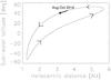 |
Fig. 1 Evolution of the subsolar latitude during one revolution of 67P around the Sun. The period of interest in this article is indicated by a bold arrow. |
Figure 1 shows the evolution of the subsolar latitude on the nucleus of 67P throughout its orbit around the Sun, assuming the current orbital and rotational parameters. The southern polar regions are subject to a short-lived, but extremely intense summer season around perihelion, after which they remain constantly shadowed from the Sun for the remainder of the comet’s orbit, in a deep winter polar night. They are thus of particular interest, and their early characterization before receiving direct sunlight in May 2015 was crucial for understanding how their activity developed and whether and how they may differ from other regions of 67P that experienced diurnal activity in August through October 2015. In addition, once these regions became illuminated in May 2015, MIRO has been able to measure and spectroscopically map the local outgassing, as has been done elsewhere on the nucleus (Gulkis et al. 2015; Biver et al. 2015; Lee et al. 2015). These more recent results are beyond the scope of this article, and will be presented and discussed elsewhere.
After the Rosetta rendezvous maneuver on August 6, 2014, spatially resolved observations of the thermal emission of 67P by MIRO were possible during four distinct trajectory phases:
- 1)
A series of arcs occurred between August 6, 2014 and September 12, 2014, to slowly reduce the distance between Rosetta and 67P from 120 to 40 km. At this range of distances, the half-power beam width (HPBW) of the SMM and MM channels yield footprints in the ranges 830−280 m (MM) and 260−90 m (SMM).
- 2)
Quasi-circular orbits around 67P followed. From the middle to the end of September 2014, the distance between Rosetta and 67P was around 29 km, yielding HPBW footprints of 200 m (MM) and 60 m (SMM).
- 3)
The distance from comet center was then decreased to ~19 km during the period of end of September to mid-October 2014, yielding HPBW footprints of 130 m (MM) and 40 m (SMM).
- 4)
The distance of Rosetta to 67P was decreased to ~9 km until the end of October 2014, yielding HPBW footprints of 70 m (MM) and 20 m (SMM).
2.2. Data acquisition and description of observations
2.2.1. Data acquisition and calibration
Raw continuum measurements for both SMM and MM channels are converted into antenna temperatures by measuring the radiance of two calibration targets every 30 min. A warm target is thermally controlled and located within MIRO, and a cold target is located outside of the spacecraft and is passively cooled. Their typical temperatures are within the ranges 290−300 K and 225−235 K, respectively. More details on the calibration of continuum measurements are reported in Gulkis et al. (2010). We here used datasets of time-stamped 1 s averages of the measurements. Corresponding geometry information (with the same time stamps) was derived from the most recent reconstructed trajectories, pointings, and the SHAP2 shape model from OSIRIS (Jorda et al. 2015) using SPICE (Acton 1996) routines.
Thermal emission data are reported as calibrated antenna temperatures for each channel. We took into account a 0.94 beam efficiency ratio between the SMM and the MM channels (Schloerb et al. 2015). The antenna temperatures TA correspond to the total power received by the MIRO continuum receivers at their frequency of operation. The wavelength dependence of the blackbody emission needs to be accounted for (e.g., Gulkis et al. 2010, 2012, and therein). The TA at a frequency ν, TA(ν), is related to the brightness temperature TB(ν) of a spatially resolved and uniform source by the following equation (Gulkis et al. 2010; Redman et al. 1992, and therein): 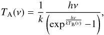 (1)where h and k are the Planck and Boltzmann constants, respectively. Equation (1) can be rearranged to derive TB from the measured antenna temperatures in the two MIRO continuum channels. In the remainder of this manuscript, we refer to either antenna or brightness temperatures, depending on whether received flux or actual subsurface temperature measurements are of primary interest.
2.2.2. Accuracy of antenna temperature measurements
Antenna temperature values on the southern polar regions experiencing deep polar night are expected to be extremely low, in the ranges 15−40 K (SMM) and 25−50 K (MM), as we show below. However, the MIRO calibration targets are at much warmer temperatures. The determination of any temperature lower than the temperature of the cold load thus relies on gain extrapolation, assuming linearity of the receivers.
Blank-sky (off-nucleus) measurements allow for testing the validity of this extrapolation. Indeed, at the frequency of the receivers in continuum mode, the coma of 67P is transparent – there are no molecular emission lines. We compiled all off-nucleus data by finding time periods where the MIRO beams were entirely located beyond the limb of 67P in the period of interest and compared the average antenna temperatures measured in each channel.
Sky antenna temperatures are within 1−2 K from expected values, which shows the accuracy of the calibration itself. The cosmic microwave background (CMB) is equivalent to an emission source with a brightness temperature of 2.7 K, which corresponds to antenna temperatures of 10-3 K (SMM) and 0.32 K (MM) (Eq. (1)). The average MIRO antenna temperatures recorded on blank sky were +1.303 K (SMM) and −0.709 K (MM), indicating that both SMM and MM sky records were offset from their expected values: the standard deviations on these measurements, of 0.746 K for the SMM and 0.341 K for the MM channels, were significantly smaller than the measured offsets. Antenna temperature values recorded on the nucleus were therefore corrected for these offsets by subtracting 1.3 K from all of the SMM and adding 1.0 K to all of the MM polar night antenna temperature measurements.
2.2.3. Observation types
MIRO has acquired continuum data continuously throughout the period of interest. The footprint of the beams is very small compared to the apparent size of the nucleus, which provides data at high spatial resolution. We used three different observation types:
-
1)
Global nucleus mapping (GNM): in this mode, MIRO controlled the pointing of the Rosetta spacecraft for preselected periods of time. GNM observations consist of controlled back-and-forth slew scans at a constant rate of 2 deg/min. The scans are typically oriented along the projection of the Sun-comet line in the XY plane of Rosetta, of which the Z-axis (which contains all instrument boresights) is the normal. In some instances, the orientation is parallel to the projection of the spin axis of 67P in the Rosetta XY plane, or perpendicular to it. Between each scan, a step by one SMM HPBW (7.5 arcmin) in the perpendicular direction is imposed to maximize coverage on 67P within each GNM period. The length of each scan was chosen to ensure that the scans extended beyond the nucleus limb (at least on one side), and thus would contain CMB sky data for calibration control.
-
2)
Nucleus gas emission (NGE): in this mode, MIRO also controlled the pointing of the Rosetta spacecraft for preselected periods of time. NGE observations consist of controlled back-and-forth slew scans at a constant rate of 0.25 deg/min. This scan rate allows for acquiring spatially resolved spectrometer data, as the MIRO CTS has an integration time of 30 s. The scans are typically oriented along the projection of the Sun-comet line in the XY plane of Rosetta (in some instances, the orientation is parallel to the projection of spin axis of 67P in the Rosetta XY plane, or perpendicular to it). The steps between scans in the orthogonal direction are on the order of 1 to 3°, depending on the size of 67P as seen from Rosetta within each NGE period, to diversify coverage on the nucleus and innermost parts of the coma. The length of each scan was chosen to ensure that the scans extended beyond the nucleus limb.
-
3)
Rider mode: in this mode, the Rosetta pointing is controlled by other instruments or reserved for spacecraft activities (navigation images, wheel off-loading, trajectory correction maneuvers). MIRO remains powered on and continuously acquires both continuum and spectroscopy data.
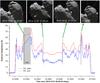 |
Fig. 2 Excerpt from MIRO GNM observation on 2014-10-23 (two consecutive scans). Top: series of images show Rosetta views of the nucleus shape of 67P at various times within the scans, obtained from the Rosetta 3D tool (ESA/Rosetta/SGS – CC BY-SA IGO 3.0). The exposure is deliberately enhanced to make shadowed region visible in the images. The MIRO beam footprints are shown as two green circles, large (MM) and small (SMM). Back-and-forth scans were made at a rate of 2 deg/min, and 1 min was allocated between scan lines for steps in the orthogonal direction. The orientation and direction of the scanning pattern is depicted with white dashed arrows in every image. Bottom: antenna temperatures (TA) recorded as a function of time over the scanning pattern. SMM and MM TA are shown in blue and red, respectively. A calibration interruption of the data is indicated by the gray shaded area denoted CAL. The exact times of Rosetta views at the top of figure are indicated as dashed vertical lines. 0 K-level sky data are obtained at the beginning of the first scan and at the end of the second. All other measurements are fully resolved, on-nucleus, and mostly cover regions that are not illuminated. |
3. Data
The observation modes described above allowed MIRO to acquire a variety of thermal emission data from southern polar night regions at various times within the period of interest. Specifically, the spacecraft trajectory regularly brought the subspacecraft point to high southern latitudes, from distances where both the SMM and MM beams could fully resolve the southern regions in polar night. We first present excerpts of MIRO data obtained during prime observation periods, from 9 km distance, to illustrate the data as obtained. Then we summarize all the polar night thermal emission data acquired during the period of interest.
3.1. Example: prime MIRO thermal emission data from 9 km distance
During the period of interest, several other opportunities for acquiring thermal emission data over the southern regions of 67P when they experienced polar night occurred at distances of 29, 19, and 9 km. A particularly interesting set of GNM observations was acquired on October 23−24, 2014. Following this set of observations, pointing was reserved for the preparation of the Philae landing. At that time, the distance from comet center was ~9 km, and the Rosetta subspacecraft point was located slightly below the equator on the nucleus. The GNM observations on October 23−24, 2014 were designed so that the scan orientation was roughly perpendicular to the spin axis of 67P, allowing optimally sampling the nucleus surface despite the short distance between Rosetta and 67P at the time of observation. The dataset provided by this GNM is unique because it consists of the most widely sampled thermal emission data on the surface of 67P, obtained with the highest spatial resolution that MIRO could achieve, during prime observation periods.
Figure 2 shows an excerpt (two consecutive scans) from this dataset. The scanning pattern was such that off-nucleus data were obtained during the 1 min latency between two scans, on one side of the nucleus only (off the large lobe). In addition, the orientation of the scans is responsible for the acquisition of thermal emission data solely on the southern regions of the nucleus, on all of its three portions: both lobes and the neck region. The Rosetta views show that many regions sampled by these scans are located in areas of 67P where the current shape model contains no information, or too little information to derive the shape reliably, and consists primarily of interpolated curvatures. This is due to the lack of illumination by the Sun on these regions during the course of the day, which suggests that these regions were experiencing a deep winter polar night at that time. The antenna temperatures recorded over non-illuminated regions span the ranges 17−40 K (SMM) and 30−50 K (MM). The first and second scans are quite symmetric, which confirms that the first scan ended over southern polar areas on the small lobe before scanning back in the other direction. The high-end values (and higher values recorded on the large lobe in portions where shape information is available) suggest some sampling of mid-southern latitude regions experiencing diurnal variations in illumination, which means that they are subject to low levels of solar flux at times during the 67P day. The low-end values are consistent with deep polar night conditions.
MIRO data acquired on the southern polar regions of 67P during the period August-October 2014.
3.2. Data obtained on southern regions in polar night
3.2.1. Summary
Table 1 summarizes the time periods where thermal emission was measured over the southern polar regions of the nucleus of 67P and includes distance from Rosetta to the center of 67P, the location on the surface (head, neck, body), the type of observation (see Sect. 2.2.2), and the approximate range of antenna temperatures recorded (within ~1 K). This table shows that MIRO has been able to acquire a well-sampled dataset on the southern polar regions of all three parts of the nucleus, from a variety of distances between Rosetta and 67P. Distance does influence the measured antenna temperatures. At the largest distances, the large size of our beam projected on the nucleus allows some spillover of flux from partially illuminated regions and results in higher temperatures than are recorded at smaller distances when the beam only samples true polar night. Table 1 shows that when the spacecraft-comet distance is shorter than 70 km, the SMM channel temperatures are all consistent, and when the distance is shorter than 30 km, the MM channels become consistent. The heliocentric distance of 67P varied from 3.5 to 3.1 AU during the period of interest. However, the subsolar latitude only changed from +45° to +40° during this period, and southern polar regions below ~−45° (45° S) remained in deep winter night throughout this period, as evidenced from the similarity in recorded temperatures once each beam fully resolved the polar night regions.
3.2.2. Data projection onto the shape model of 67P
The irregular shape of the nucleus and the lack of knowledge of the actual shape in the southern region at the time of observation are such that the SHAP2 shape model allows sunlight to reach bodycentric latitudes as high as −80° in the neck region, for example, which is unrealistic given the data acquired more recently on the southern regions. To compare our measured temperatures with thermal models, which are computed in spherical coordinates, we converted bodycentric coordinates into effective latitude. The effective latitude corresponds to the latitude at which a point would be situated if it were on a sphere. It can be calculated everywhere on the shape model because it is the angle between the surface normal of any surface element and the spin axis of 67P. Figure 3 shows effective latitude values at every point in the southern regions of the nucleus of 67P, computed using the SHAP2 model provided by the OSIRIS team (Jorda et al. 2015). The smooth variation in effective latitude from known lit regions toward the high southern latitudes, as well as the obvious large discrepancy between bodycentric latitude and effective latitude, show the current lack of information on the actual shape model.
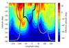 |
Fig. 3 Effective latitude values for the SHAP2 model, mapped in bodycentric latitude-longitude coordinates. The black and gray solid lines indicate the limits of the small and large lobes, respectively. |
3.2.3. Thermal mapping of the southern regions of 67P
All of the data listed in Table 1 were used to generate brightness temperature maps of the southern regions of 67P. We separated the dataset into four parts, which correspond to the four main series of distances throughout the period of interest: data acquired at a distance greater than 35 km (August and early September), then all data acquired within 35 km distance, that is, around 29 km (mid-September), then around 19 km (late September to mid-October), and around 10 km (late October). Data obtained at distances greater than 35 km are well sampled, but with poor spatial resolution for the MM channel. Data from ~29 km cover most of the nucleus. Data from ~19 and 9 km are consistent with data from larger distances, but they do not provide global coverage of 67P.
With this combination of sampling and spatial resolution limitations, we maximized the MIRO coverage of the southern regions of 67P while still preserving high spatial resolution by combining all data acquired at distances closer than 35 km from the nucleus. Brightness temperature maps were constructed by gridding the data into 5° × 5° latitude and longitude bins and averaging all brightness temperature data within each bin. When no data were available in a given bin, a local brightness temperature value of 0 K was assigned at latitudes southward of −40° (close to the polar night temperatures but below the scale), and of 120 K at latitudes northward of −40° (close to the diurnally averaged temperatures in the lit portions of the southern regions, but above the scale).
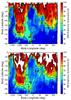 |
Fig. 4 Brightness temperature maps compiling all data obtained at distances smaller than 35 km from the comet center for the SMM (top) and MM (bottom) channels. Near-equatorial regions appear white because their temperatures are higher than the maximum value of the color scale. See text for details. |
Figure 4 shows the maps as generated. The southern regions of the nucleus of 67P appear very well sampled in this combined dataset, with spatial resolutions of ~90 and ~250 m or better for the SMM and MM channels, respectively. Most of the southern regions of 67P have not been mapped to date by any instrument other than MIRO due to the lack of illumination. Both SMM and MM data show that part of the neck region experiences fairly high temperatures (up to 90−100 K) at very high southern latitudes, which we attribute to the poor constraints on the shape model in their region. Low brightness temperatures are observed below the neck region, that is, many latitudes westward of −140° longitude (using an east longitude system), and high-latitude regions southward of −80° for longitudes between −140° and −50°; below the head region (latitudes between −10° and −40° for longitudes between −50° and +20°); and below the other part of the neck and body regions (latitudes southward of −60° for longitudes higher than +20°). Brightness temperatures in these regions are mostly within the range 25−50 K for both channels, which is a clear indication that these areas remained unlit for a significant amount of time and thus experienced deep polar night conditions.
4. Estimating the thermal properties of the southern polar regions of 67P
In this section we compare the temperatures measured by MIRO at the two wavelengths of operation with model predictions for a range of thermal inertia values.
To compare our SMM and MM brightness temperatures recorded in the southern polar regions, we selected portions of the shape model where high negative effective latitudes match very low temperatures. Indeed, temperatures higher than ~60 K in the southern polar regions experiencing polar night would require thermal inertia values that are at least one order of magnitude higher than those derived elsewhere on the nucleus, and thus appear unrealistic (Gulkis et al. 2015; Schloerb et al. 2015). We expect these temperatures to be indicative of regions where the shape model is in error. We restricted our dataset for further analysis to the following regions, expressed in bodycentric latitude-longitude coordinates: latitudes lower than −30° at longitudes west of −140° (west of the neck region); latitudes south of −80° in the neck region (longitudes between −140° and −50°); latitudes between −10° and −40° in the head region (longitudes between −50° and +20°); and latitudes south of −60° in the other part of the neck region and on the body (longitudes west of +20°).
The data were ordered in 2° effective latitude bins, within which we averaged all brightness temperature measurements for both the SMM and the MM channel. Each effective latitude bin contains on the order of ~1000 to 2000 data points, which confirms that MIRO obtained very good coverage of the southern polar regions on the nucleus and that all latitude bins are fairly uniformly sampled.
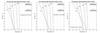 |
Fig. 5 Thermal profiles over the polar night region as a function of effective latitude (−45°, −60°, and −75°), for thermal inertia values of 5, 12, 22, 37, and 60 J m-2 K-1 s-0.5, which are hereafter compared with MIRO SMM and MM brightness temperatures. The emission depths (Le) for a regolith with lunar-like dielectric properties are indicated for both wavelengths. |
4.1. Thermophysical modeling
4.1.1. Description of the thermophysical and radiative transfer models
Production of candidate brightness temperature models for comparison with the MIRO data begins with generating temperature profiles for a pole-to-pole distribution of 35 discrete latitudes, evenly spaced in units of cosine latitude on a spherical geometry at the orbit position of the observations obtained in September 2014. For each of the 35 discrete latitudes, the one-dimensional conductive heat equation was solved numerically for a candidate range of eight constant thermal inertia values (I = 5, 8, 12, 22, 37, 60, 90, and 120 J m-2 K-1 s-0.5). The thermal computations took into account the orbital elements, obliquity, and rotation period of 67P obtained from a fit to the JPL SPICE-based ephemeris. Seasonal effects were accounted for by running the thermal model calculations over a sufficient number of orbits to achieve a periodic steady state was. Computations were stopped at the September 2014 orbit position of 67P (Sun distance ~3.4 AU), and resulting temperature profiles at 2 degree diurnal phase intervals were saved to files for each of the 35 latitudes and eight thermal inertia candidate values.
The thermal model temperature profile outputs served as inputs to a radiative transfer program that computed model brightness temperatures at the effective latitude and local hour angle of each MIRO observation by interpolation in latitude and local phase from the thermal files. The effective latitude and local hour angle were determined from the orientation of the SHAP2 model plate located at the center of the MIRO SMM and MM beams. Diurnal phase effects are absent in the polar night regions, thus the model TB results are presumably largely insensitive to electrical properties. A lunar powder model (Gary & Keihm 1978) of electrical properties was used in the radiative transfer code to compute brightness temperatures. This model is consistent with expectations based on laboratory measurements conducted on natural and comet simulant samples by Heggy et al. (2012) and Brouet et al. (2014). For more details on the thermal and radiative transfer modeling see Gulkis et al. (2010) and Schloerb et al. (2015).
4.1.2. Particularities of regions experiencing winter polar night
All regions of the nucleus of 67P experience seasonal changes in the temperature at large depths. Most regions are also subject to strong superimposed diurnal variations in insolation, which are used by combining the SMM and MM data to retrieve thermal properties (Gulkis et al. 2015; Schloerb et al. 2015). In the polar regions, however, diurnal effects disappear entirely because of the high obliquity of 67P. In the southern polar regions, this yields a winter polar night that lasts for most of the orbit. In addition to cooling these regions to extremely low temperatures, this peculiarity strongly influences the thermal profiles as function of depth and allows MIRO to be sensitive to seasonal effects in the polar regions.
Figure 5 shows the thermal profiles derived from model computations for five constant thermal inertia models, which encompass a plausible range of thermal properties (thermal inertia of 5, 12, 22, 37, and 60 J m-2 K-1 s-0.5) at three effective latitudes (−45°, −60°, and −75°). Several features can be identified in these profiles. Overall, the lower the thermal inertia, the lower the temperature within the range of depths to which MIRO is sensitive. Thermal gradients do exist, but are extremely small and vary inversely with the thermal inertia: between ~1 K/cm for thermal inertia of 5 J m-2 K-1 s-0.5 and ~0.1 K/cm for thermal inertia of 60 J m-2 K-1 s-0.5.
The emission depths (electrical penetration depths, Le) at the two frequencies of operation of MIRO for lunar-like dielectric properties are also indicated in Fig. 5. At first order, the brightness temperatures expected for a given set of thermal properties correspond to the temperature at the emission depths. Schloerb et al. (2015) showed for the sunlit regions of 67P that dielectric properties resulting in emission depths corresponding to one to two thirds of the nominal model best match diurnal MIRO SMM and MM data. In the following analysis we therefore used electrical penetration depths of 1 and 3 cm for the SMM and MM channels, respectively, for the radiative transfer model. Nevertheless, Fig. 5 shows that electrical penetration depth values within the first ~5 cm would only affect the predicted brightness temperatures by a few K at the very most, in the case of extremely low thermal inertia values.
Thus, on one hand the thermophysical models suggest that the southern polar regions of 67P are an ideal place to derive thermal properties because the modeled brightness temperatures will be relatively insensitive to the dielectric properties. On the other hand, the lack of information of the shape model in these unlit regions affects the accuracy of the determination of effective latitude positions of polar night regions, which also affect the modeled brightness temperatures.
4.2. Comparison between brightness temperature data and model predictions
We compared brightness temperature data and modeled brightness temperatures over the southern regions of 67P for the entire period of interest. We used the effective latitude binning process described in Sect. 4 to select data that are most likely to be representative of polar night conditions from our dataset. The data-model comparison is shown in Fig. 6, with error bars representing the standard error of the dataset within each bin.
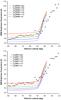 |
Fig. 6 Comparison between brightness temperature data acquired and predicted based on thermophysical and radiative transfer models assuming constant properties, for the SMM (top, 1 cm penetration depth) and MM (bottom, 3 cm penetration depth) channels. |
Based on Fig. 6, the MIRO SMM and MM data at effective latitudes corresponding to polar night conditions appear to be best fit by thermal inertia values within the ranges ~10−40 J m-2 K-1 s-0.5 and ~20−60 J m-2 K-1 s-0.5, respectively. At first order, these values are comparable with thermal inertia values inferred by Gulkis et al. (2015) and Schloerb et al. (2015) on the sunlit regions of the nucleus. Two differences can be pointed out, however: 1) the range of admissible thermal inertias extends to higher values for both channels; and 2) there is a noticeable difference between the SMM and MM results, given the small error bars.
We compare in Fig. 7 the difference in measured brightness temperatures ΔTB between the MM and the SMM channels with the ΔTB predicted by the models. Interestingly, the measured difference in brightness temperatures between the two channels is significantly larger than expected when one assumes the set of dielectric properties that best fit the sunlit side of 67P (Schloerb et al. 2015). Lower thermal inertia models seem favored by this comparison, which is a priori in contradiction with the results obtained on the individual channels. However, it must be borne in mind that the difference in brightness temperature is overall small: 3.4 K on average at effective latitudes lower than −45°, with a fairly large standard deviation of 2.5 K. Some of this difference may in part be due to instrumental effects (calibration, beam efficiency). These effects have been accounted for as best possible, however. This result thus hints at some characteristics of the nucleus that the best-fit model to the sunlit side does not reproduce.
5. Discussion
One possibility to explain a difference in the constrained thermal inertia between the SMM and MM channels could be the presence of ice(s) in significant fractions. Indeed, water ice has a very low absorbance in the microwave region. At the MIRO wavelengths and temperatures near 100 K, laboratory measurements and model predictions of pure ice indicate absorption losses 5−20 times lower than the values for lunar dust (Bertie et al. 1969; Hufford 1991; Jiang & Wu 2004).
With these low absorption losses, the electrical penetration depths could be as high as 30 cm and 100 cm at the SMM and MM frequencies, respectively, approximately twenty times the lunar model values. Thus, if ice is indeed present in significant fractions, the MIRO brightness temperatures may correspond to temperatures from much deeper layers of the southern polar regions.
We used a chi-square minimization scheme to find the values of electrical penetration depth that provide best fits of the polar night data (effective latitudes southward of −45° only) for each thermal inertia model to both the individual channel data and the difference in brightness temperature.
The thermal profiles in the southern polar regions plotted in Fig. 5 show that small positive thermal gradients exist with depth, therefore we only considered thermal models with inertia values lower than 60 J m-2 K-1 s-0.5 in the fitting process: the deeper the penetration depth, the higher the brightness temperature in such thermal environments. Therefore the models with higher thermal inertias (90 and 120 J m-2 K-1 s-0.5) cannot provide a good fit to the data.
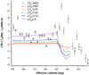 |
Fig. 7 Difference in measured brightness temperatures between the MM and SMM channels compared with thermophysical model predictions. Data are shown as open circles. |
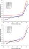 |
Fig. 8 Comparison between brightness temperature data acquired and predicted based on thermophysical and radiative transfer models assuming constant thermal properties and best-fit electrical penetration depths for the SMM (top) and MM (bottom) channels. |
Figure 8 shows these best-fit brightness temperature models. Best fits are found for the SMM channel for electrical penetration depths ~15–20 cm for thermal inertias between 5 and 22 J m-2 K-1 s-0.5, and a shallower-than-nominal electrical penetration for a thermal inertia of 37 J m-2 K-1 s-0.5. For the MM data, best fits are obtained for penetration depths of ~20–30 cm for thermal inertias of 5 to 37 J m-2 K-1 s-0.5. This wide range of best-fit electrical penetration depths shows that the polar night regions are weakly sensitive to the electrical properties, as expected. However, this range also suggests that the polar night data recorded by MIRO could indicate the presence of a significant fraction of ice(s) within the subsurface.
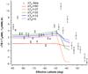 |
Fig. 9 Difference in measured brightness temperatures between the MM and SMM channels compared with thermophysical model predictions using best-fit electrical penetration depths from the chi-square minimization scheme for each channel. Data are shown as open circles. See text for details. |
Thus, we hypothesize that the southern polar regions may contain ice(s) on the surface or the shallow subsurface (first tens of centimeters). Ice(s) in these regions might have formed upon cooling after the previous perihelion passage of 67P in these parts of the nucleus: effectively, the southern polar regions would act as a cold trap and would become enriched in ice(s), which may increase thermal contact between grains and therefore increase the thermal inertia derived from the measurements and decrease their absorptivity at the MIRO frequencies.
In addition, significantly greater penetration depths than the nominal case allow better reproducing the measured differences in brightness temperatures between the two channels ΔTB, as shown in Fig. 9. This figure confirms that thermal models with low thermal inertias can provide best fits to the data owing to their extremely great penetration depths. It also provides further support for our hypothesis that over the seasonal timescales that MIRO can observe in the polar regions, the presence and amounts of ice present on the surface and within the first tens of centimeters drive the dielectric properties.
It must be borne in mind that this hypothesis is currently relying on the poorly known shape of the nucleus of 67P in these regions and thus is a speculation. Nevertheless, the difference in brightness temperatures ΔTB is quite insensitive to the uncertainty on the shape model because it directly compares SMM and MM measurements from the same location on 67P. This, in addition to the result that models which include very great penetration depths provide best fits to both the individual channels and the ΔTB, further supports our hypothesis.
Rosetta has continuously acquired data in the southern polar regions of 67P since the period considered in this article, and MIRO and other Rosetta instruments will use these new data to better constrain the shape, the thermal environment, and the possible presence and abundance of ice(s) that is suggested by the data presented herein.
6. Conclusions
We presented MIRO continuum observations of the southern regions of 67P acquired between August and October 2014 from a range of distances. These data were compared with predicted brightness temperatures from thermophysical and radiative transfer models. Our main findings are as follows:
-
Deep winter conditions occurred during the period of interest in the three southern polar regions: neck, small lobe, and large lobe.
-
Thermal inertias within the ranges 10−40 (SMM) and 20−60 (MM) J m-2 K-1 s-0.5 match our data for the southern polar regions, and no indication of differences between the three regions (two lobes and neck) was found from a thermal properties perspective.
-
The difference in best-fit thermal inertias between the two channels, as well as possible great electrical penetration depths that match the obtained data much better than the nominal model, are suggestive of the presence of ice(s) within the shallow subsurface of these regions.
Acknowledgments
Part of this work has been conducted at the Jet Propulsion Laboratory, California Institute of Technology, under contract to the National Aeronautics and Space Administration (NASA). Part of the research was carried out at the Max-Planck-Institut für Sonnensystemforschung with financial support from Deutsches Zentrum für Luft- und Raumfahrt and Max-Planck-Gesellschaft. Parts of the research were carried out by LESIA and LERMA, Observatoire de Paris, with financial support from CNES and CNRS/Institut des Sciences de l’Univers. Part of the research was carried out at the National Central University with funding from the Taiwanese National Science Counsel grant NSC 101-2111-M-008-016. Part of the research was carried out at the University of Massachusetts, Amherst, USA. Support from ESA’s Rosetta Mission Operations Control center and ESA’s Rosetta Science Ground Segment, for preparation and implementation of the observations, and communication of the acquired data, is gratefully acknowledged. The authors thank the ESA/Rosetta/SGS team for permission to use output from their 3D tool (CC BY-SA IGO 3.0). We thank Y. Anderson, T. Koch, R. Nowicki, L. Pan and the late Lucas Kamp for their efforts in scheduling, operations, and support of the MIRO instrument. Financial support from the US Rosetta Project and government sponsorship are acknowledged.
References
- Acton, C. H. 1996, Planet. Space Sci., 44, 65 [NASA ADS] [CrossRef] [Google Scholar]
- Bertie, J., Labbe, H., & Whalley, E. 1969, J. Chem. Phys., 50, 4501 [NASA ADS] [CrossRef] [Google Scholar]
- Biver, N., Hofstadter, M., Gulkis, S., et al. 2015, A&A, 583, A3 [NASA ADS] [CrossRef] [EDP Sciences] [Google Scholar]
- Brouet, Y., Levasseur-Regourd, A., Encrenaz, P., & Gulkis, S. 2014, Planet. Space Sci., 103, 143 [NASA ADS] [CrossRef] [Google Scholar]
- Gary, B. L., & Keihm, S. J. 1978, Lunar and Planetary Science Conf. Proc., 9, 2885 [NASA ADS] [Google Scholar]
- Gulkis, S., Frerking, M., Crovisier, J., et al. 2007, Space Sci. Rev., 128, 561 [NASA ADS] [CrossRef] [Google Scholar]
- Gulkis, S., Keihm, S., Kamp, L., et al. 2010, Planet. Space Sci., 58, 1077 [NASA ADS] [CrossRef] [Google Scholar]
- Gulkis, S., Keihm, S., Kamp, L., et al. 2012, Planet. Space Sci., 66, 31 [NASA ADS] [CrossRef] [Google Scholar]
- Gulkis, S., Allen, M., von Allmen, P., et al. 2015, Science, 347, aaa0709 [Google Scholar]
- Heggy, E., Palmer, E. M., Kofman, W., et al. 2012, Icarus, 221, 925 [NASA ADS] [CrossRef] [Google Scholar]
- Hufford, G. 1991, Int. J. Infrared and Millimeter Waves, 12, 677 [Google Scholar]
- Jiang, J. H., & Wu, D. L. 2004, Atmos. Sci. Lett., 5, 146 [NASA ADS] [CrossRef] [Google Scholar]
- Jorda, L., Gaskell, R., Hviid, S. L., et al. 2015, NASA Planetary Data System and ESA Planetary Science Archive [Google Scholar]
- Krolikowska, M. 2003, Acta Astron., 53, 195 [NASA ADS] [Google Scholar]
- Lamy, P. L., Toth, I., Davidsson, B. J., et al. 2007, Space Sci. Rev., 128, 23 [NASA ADS] [CrossRef] [Google Scholar]
- Lee, S., von Allmen, P., Allen, M., et al. 2015, A&A, 583, A5 [NASA ADS] [CrossRef] [EDP Sciences] [Google Scholar]
- Redman, R. O., Feldman, P., Matthews, H., Halliday, I., & Creutzberg, F. 1992, AJ, 104, 405 [NASA ADS] [CrossRef] [Google Scholar]
- Schloerb, F. P., Keihm, S., von Allmen, P., et al. 2015, A&A, 583, A29 [NASA ADS] [CrossRef] [EDP Sciences] [Google Scholar]
- Schulz, R. 2009, Sol. Sys. Res., 43, 343 [Google Scholar]
- Sierks, H., Barbieri, C., Lamy, P. L., et al. 2015, Science, 347, aaa1044 [Google Scholar]
All Tables
MIRO data acquired on the southern polar regions of 67P during the period August-October 2014.
All Figures
|
Fig. 1 Evolution of the subsolar latitude during one revolution of 67P around the Sun. The period of interest in this article is indicated by a bold arrow. |
| In the text | |
|
Fig. 2 Excerpt from MIRO GNM observation on 2014-10-23 (two consecutive scans). Top: series of images show Rosetta views of the nucleus shape of 67P at various times within the scans, obtained from the Rosetta 3D tool (ESA/Rosetta/SGS – CC BY-SA IGO 3.0). The exposure is deliberately enhanced to make shadowed region visible in the images. The MIRO beam footprints are shown as two green circles, large (MM) and small (SMM). Back-and-forth scans were made at a rate of 2 deg/min, and 1 min was allocated between scan lines for steps in the orthogonal direction. The orientation and direction of the scanning pattern is depicted with white dashed arrows in every image. Bottom: antenna temperatures (TA) recorded as a function of time over the scanning pattern. SMM and MM TA are shown in blue and red, respectively. A calibration interruption of the data is indicated by the gray shaded area denoted CAL. The exact times of Rosetta views at the top of figure are indicated as dashed vertical lines. 0 K-level sky data are obtained at the beginning of the first scan and at the end of the second. All other measurements are fully resolved, on-nucleus, and mostly cover regions that are not illuminated. |
| In the text | |
|
Fig. 3 Effective latitude values for the SHAP2 model, mapped in bodycentric latitude-longitude coordinates. The black and gray solid lines indicate the limits of the small and large lobes, respectively. |
| In the text | |
|
Fig. 4 Brightness temperature maps compiling all data obtained at distances smaller than 35 km from the comet center for the SMM (top) and MM (bottom) channels. Near-equatorial regions appear white because their temperatures are higher than the maximum value of the color scale. See text for details. |
| In the text | |
|
Fig. 5 Thermal profiles over the polar night region as a function of effective latitude (−45°, −60°, and −75°), for thermal inertia values of 5, 12, 22, 37, and 60 J m-2 K-1 s-0.5, which are hereafter compared with MIRO SMM and MM brightness temperatures. The emission depths (Le) for a regolith with lunar-like dielectric properties are indicated for both wavelengths. |
| In the text | |
|
Fig. 6 Comparison between brightness temperature data acquired and predicted based on thermophysical and radiative transfer models assuming constant properties, for the SMM (top, 1 cm penetration depth) and MM (bottom, 3 cm penetration depth) channels. |
| In the text | |
|
Fig. 7 Difference in measured brightness temperatures between the MM and SMM channels compared with thermophysical model predictions. Data are shown as open circles. |
| In the text | |
|
Fig. 8 Comparison between brightness temperature data acquired and predicted based on thermophysical and radiative transfer models assuming constant thermal properties and best-fit electrical penetration depths for the SMM (top) and MM (bottom) channels. |
| In the text | |
|
Fig. 9 Difference in measured brightness temperatures between the MM and SMM channels compared with thermophysical model predictions using best-fit electrical penetration depths from the chi-square minimization scheme for each channel. Data are shown as open circles. See text for details. |
| In the text | |
Current usage metrics show cumulative count of Article Views (full-text article views including HTML views, PDF and ePub downloads, according to the available data) and Abstracts Views on Vision4Press platform.
Data correspond to usage on the plateform after 2015. The current usage metrics is available 48-96 hours after online publication and is updated daily on week days.
Initial download of the metrics may take a while.