© ESO, 2015

1. Introduction

Transverse oscillations of magnetic loops in the solar corona have been under intense research since the first observational reports by the Transition Region And Coronal Explorer (TRACE) (see, e.g., Nakariakov et al. 1999; Aschwanden et al. 1999). Large-amplitude coronal loop oscillations are usually excited after energetic events such as solar flares, coronal mass ejections, or low coronal eruptions (see Zimovets & Nakariakov 2015). Based on magnetohydrodynamic (MHD) wave theory (e.g., Nakariakov & Verwichte 2005), transverse loop oscillations have been interpreted as standing kink MHD waves. Kink MHD modes are nearly incompressible waves, mainly driven by magnetic tension, and responsible for global transverse motions of the flux tube (see, e.g., Edwin & Roberts 1983; Goossens et al. 2009, 2012). A relevant feature of large-amplitude loop oscillations is that they are strongly damped. It has been shown that resonant absorption, caused by plasma inhomogeneity in the direction perpendicular to the magnetic field, is an efficient damping mechanism of kink MHD waves in coronal loops (see, e.g., Ruderman & Roberts 2002; Goossens et al. 2002). Because of resonant absorption, the energy from the global kink motion of the flux tube is transferred to small-scale, unresolved rotational motions around the nonuniform boundary of the tube (see, e.g., Terradas et al. 2006; Goossens et al. 2014; Soler & Terradas 2015). As a result of this process, the global kink oscillation of the coronal loop is quickly damped in time. The interested reader is referred to Goossens et al. (2011), where the theory and applications of resonant waves in the solar atmosphere are reviewed.

Observations often show that neighboring oscillating loops in an active region interact with each other and exhibit collective behavior (e.g., Schrijver & Brown 2000; Verwichte et al. 2004; Schrijver et al. 2002; White et al. 2013). Interaction between loops can modify the properties of their transverse oscillations with respect to the properties of the classic kink mode of an isolated loop. Therefore, advanced models describing coronal loop oscillations should take into account interactions within loop systems. A number of works have studied collective transverse oscillations in Cartesian geometry (e.g., Díaz et al. 2005; Díaz & Roberts 2006; Luna et al. 2006; Arregui et al. 2007, 2008). In cylindrical geometry, Luna et al. (2008) numerically investigated transverse oscillations of two cylindrical loops, and Ofman (2009) performed numerical simulations in the case of four interacting loops. Concerning analytical works in cylindrical geometry, Luna et al. (2009, 2010) used the T-matrix theory of scattering (see, e.g., Twersky 1952; Waterman 1969; Bogdan 1987; Keppens et al. 1994) to investigate transverse oscillations of two and three loops (Luna et al. 2009) and of bundles of many loops (Luna et al. 2010) in the β = 0 approximation, where β refers to the ratio of the gas pressure to the magnetic pressure. Soler et al. (2009) later extended the method of Luna et al. (2009, 2010) by incorporating gas pressure and longitudinal flows and studied collective oscillations of flowing prominence threads. These works showed that loop interaction affects the properties of their oscillations. Luna et al. (2008, 2009) found that a system of two loops of arbitrary radii supports four kink-like collective modes. The shift of the collective mode frequencies with respect to the individual kink frequencies of the loops is significant when the distance between loops is small (approximately the size of the loop radius) and when loops have similar densities. Conversely, the oscillating loops show little interaction when they are far from each other and when their densities are substantially different. On the other hand, Van Doorsselaere et al. (2008) and Robertson et al. (2010) used a different method based on bycilindrical coordinates to study transverse oscillations of two pressureless loops in the thin tube (TT) approximation. Of the four kink-like collective modes obtained by Luna et al. (2009) in the T-matrix theory, only two different modes remain in the TT approximation considered by Van Doorsselaere et al. (2008) and Robertson et al. (2010).

Concerning the damping of the oscillations, Arregui et al. (2007, 2008) investigated resonantly damped oscillations of two slabs, while Terradas et al. (2008) numerically studied the resonant damping of transverse oscillations of a multi-stranded loop. Those works showed that the process of resonant damping is not compromised by the irregular geometry of a realistic loop model and still produces the efficient attenuation of global transverse oscillations. The damping of transverse oscillations of two cylindrical loops was analytically investigated by Robertson & Ruderman (2011) and Gijsen & Van Doorsselaere (2014), who considered the TT approximation and used bycilindrical coordinates. Results obtained with bycilindrical coordinates should be treated with caution when the distance between loops is small. Geometrical effects intrinsically associated with the bycilindrical coordinates may produce unphysical results. Our purpose is to use the T-matrix method of Luna et al. (2009, 2010) to investigate resonantly damped oscillations of bundles of loops. The present paper is partially based on unpublished results included in Soler (2010)¹. The effect of resonant absortion in the Alfvén continuum is incorporated to the T-matrix scheme by using the method that combines the jump conditions of the perturbations at the resonance position with the so-called thin boundary (TB) approximation (see, e.g., Sakurai et al. 1991; Goossens et al. 1992). A similar method was previously used by Keppens (1995) to investigate absorption of acoustic waves. We provide a general analytic theory, which is valid for bundles of many transversely nonuniform parallel loops of arbitrary radii. Specific results in the case of two loops are obtained and compared to those given in Robertson & Ruderman (2011) and Gijsen & Van Doorsselaere (2014). Our results are also compared to those of Arregui et al. (2007, 2008) obtained in Cartesian geometry.

This paper is organized as follows. Section 2 contains the description of the equilibrium configuration and the basic governing equations. The general analytic T-matrix theory of scattering to compute the frequencies and damping rates of collective loop oscillations is given in Sect. 3. Later, the specific case of damped oscillations of two loops is discussed both analytically and numerically in Sect. 4. Finally, some concluding remarks are given in Sect. 5.

2. Model and governing equations

Our equilibrium configuration is composed of N straight and parallel magnetic cylinders of length L embedded in a uniform coronal plasma. The ends of the magnetic tubes are fixed at two rigid walls representing the solar photosphere. We set the z-direction to be along the axes of the tubes. The magnetic field is straight along the z-direction, namely B = Bê_z, where B is a constant everywhere. We use the subscripts “i” and “e” to refer to, in general, the internal region of the tubes and the external plasma, respectively. The subscript or superscript “j” is used to refer to a particular loop. We denote by R_j the radius of the jth tube. The distance between the centers of the jth and j’th loops is d_jj′. We denote by ρ_j the internal density of the jth tube, while ρ_e denotes the external density, i.e., the density of the coronal environment. In our model ρ_j and ρ_e are constants. There is a transversely nonuniform transitional layer surrounding each magnetic tube in which the density continuously varies from the internal density, ρ_j, to the external density, ρ_e. The thicknesses of the nonuniform boundary layer of the jth cylinter is l_j. A sketch of the equilibrium configuration in the case of two magnetic tubes (N = 2) is given in Fig. 1.

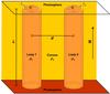Fig. 1 Sketch of the equilibrium configuration in the specific case of two transversely nonuniform coronal loops.

We adopt the β = 0 approximation, where β refers to the ratio of the thermal pressure to the magnetic pressure. This is an appropriate approximation to investigate transverse waves in the solar corona. In the β = 0 approximation, the ideal MHD equations governing linear perturbations superimposed on the static equilibrium state are $\begin{array}{ccc}& & \mathit{\rho }\frac{{\mathit{\partial }}^{\mathrm{2}}{\xi }}{\mathit{\partial }{\mathit{t}}^{\mathrm{2}}}\mathrm{=}\frac{\mathrm{1}}{\mathit{\mu }}\left(\mathrm{\nabla }\mathrm{\times }{b}\right)\mathrm{\times }{B}\mathit{,}\\ & & {b}\mathrm{=}\mathrm{\nabla }\mathrm{\times }\left({\xi }\mathrm{\times }{B}\right)\mathit{,}\end{array}$where ξ is the plasma Lagrangian displacement, b is the magnetic field Eulerian perturbation, ρ is the density, and μ is the magnetic permittivity.

We assume the temporal dependence of perturbations as exp(−iωt), where ω is the oscillation frequency. In the case of transversely nonuniform tubes, the global transverse oscillations are quasi-modes whose frequency is complex owing to damping by resonant absorption, i.e., ω = ω_R + iω_I, where ω_R and ω_I are the real and imaginary parts of the frequency, respectively. The real part of ω is related to the period and the imaginary part corresponds to the damping rate of the oscillations. We consider that the oscillating flux tubes are line-tied at the photosphere, which acts as a perfectly reflecting wall in this model because its density is much higher than the coronal density. Hence, we assume perturbations to be proportional to exp(ik_zz), with k_z the longitudinal wavenumber. For standing oscillations, k_z given by ${\mathit{k}}_{\mathit{z}}\mathrm{=}\frac{\mathit{n\pi }}{\mathit{L}}\mathit{,} \mathrm{with} \mathit{n}\mathrm{=}\mathrm{1}\mathit{,}\mathrm{2}\mathit{,}\mathit{...}$(3)We shall restict ourselves to the fundamental mode of oscillation, so we take n = 1.

In the regions with constant density, Equations (1) and (2) can be reduced to following equation, ${\mathrm{\nabla }}_{\mathrm{\perp }}^{\mathrm{2}}{\mathit{P}}^{\mathrm{\prime }}\mathrm{+}{\mathit{k}}_{\mathrm{\perp }}^{\mathrm{2}}{\mathit{P}}^{\mathrm{\prime }}\mathrm{=}\mathrm{0}\mathit{,}$(4)where P′ = B·b/μ is the total pressure Eulerian pertubation and the subscript ⊥ refers to the direction perpendicular to the magnetic field. Thus, ${\mathrm{\nabla }}_{\mathrm{\perp }}^{\mathrm{2}}$ denotes the perpendicular part of the ∇² operator. In turn, the quantity k_⊥ plays the role of the perpendicular wavenumber and is defined as ${\mathit{k}}_{\mathrm{\perp }}^{\mathrm{2}}\mathrm{=}\frac{{\mathit{\omega }}^{\mathrm{2}}\mathrm{-}{\mathit{\omega }}_{\mathrm{A}}^{\mathrm{2}}}{{\mathit{v}}_{\mathrm{A}}^{\mathrm{2}}}\mathit{,}$(5)where ${\mathit{\omega }}_{\mathrm{A}}^{\mathrm{2}}\mathrm{=}{\mathit{k}}_{\mathit{z}}^{\mathrm{2}}{\mathit{v}}_{\mathrm{A}}^{\mathrm{2}}$ is the square of the Alfvén frequency and ${\mathit{v}}_{\mathrm{A}}^{\mathrm{2}}\mathrm{=}{\mathit{B}}^{\mathrm{2}}\mathit{/}\mathit{\mu \rho }$ is the square of the Alfvén velocity. We stress that Eq. (4) is only valid in the regions with constant density, so it does not apply within the nonuniform boundaries of the loops.

3. T-matrix theory of scattering

Equation (4) is the two-dimensional Helmholtz equation. To solve Eq. (4) we use the scattering theory in its T-matrix formalism (see, e.g., Waterman 1969). In the solar context, the T-matrix theory has previously been used to investigate the scattering and absorption properties of bundles of magnetic flux tubes (e.g., Bogdan & Zweibel 1985; Bogdan & Cattaneo 1989; Keppens et al. 1994; Keppens 1995, among others). Luna et al. (2009, 2010) used of this technique to compute the eigenmodes of systems of magnetic tubes. Because of the inhomogeneity of the tubes in the transverse direction, the modes with frequencies between the internal Alfvén frequencies of the loops and the external Alfvén frequency are resonant in the Alfvén continuum. As a result, the oscillations are damped by resonant absorption. The effect of resonant absorption was not considered by Luna et al. (2009, 2010). Here we extend their theory to consider resonant damping.

3.1. Solutions in the internal and external plasmas

We use local polar coordinates associated with the jth loop. We denote by r_j and ϕ_j the radial and azimuthal coordinates, respectively, of the coordinate system whose origin is located at the center of the jth tube. We can define an equivalent coordinate system in each tube. In this local coordinate system, the solution to Eq. (4) in the internal region of the jth tube can be expressed as ${\mathit{P}}_{\mathrm{i}}^{\mathrm{\prime }\mathit{j}}\mathrm{=}\sum _{\mathit{m}\mathrm{=}\mathrm{-}\mathrm{\infty }}^{\mathrm{\infty }}{\mathit{A}}_{\mathit{m}}^{\mathit{j}}{\mathit{J}}_{\mathit{m}}\mathrm{\left(}{\mathit{k}}_{\mathrm{\perp }\mathit{j}}{\mathit{r}}_{\mathit{j}}\mathrm{\right)}\exp \mathrm{\left(}\mathrm{i}\mathit{m}{\mathit{\varphi }}_{\mathit{j}}\mathrm{\right)}\mathit{,}$(6)where m is the azimuthal wavenumber, J_m is the usual Bessel function of the first kind of order m, and ${\mathit{A}}_{\mathit{m}}^{\mathit{j}}$ are constants. Unlike the case of isolated tubes (see, e.g., Edwin & Roberts 1983), the solution is not entirely described by a single value of m. Because of interaction between tubes, the values of m are coupled. For transverse, kink-like oscillations the dominant terms in the expansion are those with m = ± 1, but the contribution from other m’s is not negligible unless the tubes are far from each other (Luna et al. 2009).

The solution to Eq. (4) in the external region is written using the principle of superposition, which is applicable to linear waves. The total external solution is computed by adding the net contributions of all flux tubes, namely${\mathit{P}}_{\mathrm{e}}^{\mathrm{\prime }}\mathrm{=}\sum _{\mathit{j}}{\mathit{P}}_{\mathrm{e}}^{\mathrm{\prime }\mathit{j}}\mathit{,}$(7)where ${\mathit{P}}_{\mathrm{e}}^{\mathrm{\prime }\mathit{j}}$ is the net contribution of the jth tube to the external solution. The central idea behind the scattering theory is that the solution of Eq. (4) in the external plasma can be decomposed into several fields with different physical meanings, namely the total, exciting, and scattered fields. Here we give an overview of the method. Interested readers are referred to Luna et al. (2009, 2010) for extensive explanations.

In the external plasma, the total field associated with the jth cylinder can be expressed as${\mathit{P}}_{\mathrm{total}}^{\mathrm{\prime }\mathit{j}}\mathrm{=}\sum _{\mathit{m}\mathrm{=}\mathrm{-}\mathrm{\infty }}^{\mathrm{\infty }}\mathrm{[}{\mathit{\alpha }}_{\mathrm{1}\mathit{m}}^{\mathit{j}}{\mathit{H}}_{\mathit{m}}^{\mathrm{\left(}\mathrm{1}\mathrm{\right)}}\mathrm{\left(}{\mathit{k}}_{\mathrm{\perp }\mathrm{e}}{\mathit{r}}_{\mathit{j}}\mathrm{\right)}\mathrm{+}{\mathit{\alpha }}_{\mathrm{2}\mathit{m}}^{\mathit{j}}{\mathit{H}}_{\mathit{m}}^{\mathrm{\left(}\mathrm{2}\mathrm{\right)}}{\mathrm{\left(}{\mathit{k}}_{\mathrm{\perp }\mathrm{e}}{\mathit{r}}_{\mathit{j}}\mathrm{\right)}}^{\mathrm{]}}\exp \mathrm{\left(}\mathrm{i}\mathit{m}{\mathit{\varphi }}_{\mathit{j}}\mathrm{\right)}\mathit{,}$(8)where ${\mathit{H}}_{\mathit{m}}^{\mathrm{\left(}\mathrm{1}\mathrm{\right)}}$ and ${\mathit{H}}_{\mathit{m}}^{\mathrm{\left(}\mathrm{2}\mathrm{\right)}}$ are the usual Hankel functions of the first and second kind, respectively, and ${\mathit{\alpha }}_{\mathrm{1}\mathit{m}}^{\mathit{j}}$ and ${\mathit{\alpha }}_{\mathrm{2}\mathit{m}}^{\mathit{j}}$ constants. The first term on the right-hand side of Eq. (8) represents outgoing waves from the jth tube, and the second term represents incoming waves toward the jth tube. Importantly, we note that${\mathit{P}}_{\mathrm{e}}^{\mathrm{\prime }}\ne \sum _{\mathit{j}}{\mathit{P}}_{\mathrm{total}}^{\mathrm{\prime }\mathit{j}}\mathit{.}$(9)The reason for this inequality is that the outgoing wave associated with a particular tube contributes as an incoming wave for all the other tubes. In other words, ${\sum }_{\mathit{j}}{\mathit{P}}_{\mathrm{total}}^{\mathrm{\prime }\mathit{j}}$ is not the net external solution. To overcome this problem, the total field associated with the jth cylinder, ${\mathit{P}}_{\mathrm{total}}^{\mathrm{\prime }\mathit{j}}$, is decomposed into a scattered field, ${\mathit{P}}_{\mathrm{scat}}^{\mathrm{\prime }\mathit{j}}$, and a exciting field, ${\mathit{P}}_{\mathrm{excit}}^{\mathrm{\prime }\mathit{j}}$. Conceptually, the scattered field represents the actual contribution of the various tubes to the net external solution, whereas the exciting field can be understood as the cross-talk mechanism responsible for interaction between flux tubes (see details in, e.g., Bogdan & Cattaneo 1989).

The full net external solution, ${\mathit{P}}_{\mathrm{e}}^{\mathrm{\prime }}$, is defined so that it corresponds to the sum of the scattered fields associated with all tubes, namely 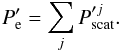${\mathit{P}}_{\mathrm{e}}^{\mathrm{\prime }}\mathrm{=}\sum _{\mathit{j}}{\mathit{P}}_{\mathrm{scat}}^{\mathrm{\prime }\mathit{j}}\mathit{.}$(10)Conversely, the exciting field associated with the jth tube is defined as the difference between the full net contribution and the scattered field of the jth tube, namely 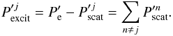${\mathit{P}}_{\mathrm{excit}}^{\mathrm{\prime }\mathit{j}}\mathrm{=}{\mathit{P}}_{\mathrm{e}}^{\mathrm{\prime }}\mathrm{-}{\mathit{P}}_{\mathrm{scat}}^{\mathrm{\prime }\mathit{j}}\mathrm{=}\sum _{\mathit{n}\ne \mathit{j}}{\mathit{P}}_{\mathrm{scat}}^{\mathrm{\prime }\mathit{n}}\mathit{.}$(11)Waterman (1969) introduced the T-matrix operator, T^j, which linearly relates the scattered and exciting fields as 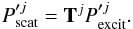${\mathit{P}}_{\mathrm{scat}}^{\mathrm{\prime }\mathit{j}}\mathrm{=}{{T}}^{\mathit{j}}{\mathit{P}}_{\mathrm{excit}}^{\mathrm{\prime }\mathit{j}}\mathit{.}$(12)Bogdan (1987) showed that for cylindrical scatterers the T-matrix is diagonal, and Keppens et al. (1994) gave an expression of its elements, namely 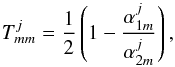${\mathit{T}}_{\mathit{mm}}^{\mathit{j}}\mathrm{=}\frac{\mathrm{1}}{\mathrm{2}}\left(\mathrm{1}\mathrm{-}\frac{{\mathit{\alpha }}_{\mathrm{1}\mathit{m}}^{\mathit{j}}}{{\mathit{\alpha }}_{\mathrm{2}\mathit{m}}^{\mathit{j}}}\right)\mathit{,}$(13)where ${\mathit{\alpha }}_{\mathrm{1}\mathit{m}}^{\mathit{j}}$ and ${\mathit{\alpha }}_{\mathrm{2}\mathit{m}}^{\mathit{j}}$ are the same constants the appear in Eq. (8). We can use Eq. (13) to eliminate ${\mathit{\alpha }}_{\mathrm{1}\mathit{m}}^{\mathit{j}}$ and write all the expressions in terms of ${\mathit{\alpha }}_{\mathrm{2}\mathit{m}}^{\mathit{j}}$ alone. With the help of these last formulae, and after some algebraic manipulations using well-known properties of the Bessel functions, we can rewrite Eq. (8) as${\mathit{P}}_{\mathrm{total}}^{\mathrm{\prime }\mathit{j}}\mathrm{=}\sum _{\mathit{m}\mathrm{=}\mathrm{-}\mathrm{\infty }}^{\mathrm{\infty }}\mathrm{2}{\mathit{\alpha }}_{\mathrm{2}\mathit{m}}^{\mathit{j}}\mathrm{[}{\mathit{J}}_{\mathit{m}}\mathrm{\left(}{\mathit{k}}_{\mathrm{\perp }\mathrm{e}}{\mathit{r}}_{\mathit{j}}\mathrm{\right)}\mathrm{-}{\mathit{T}}_{\mathit{mm}}^{\mathit{j}}{\mathit{H}}_{\mathit{m}}^{\mathrm{\left(}\mathrm{1}\mathrm{\right)}}{\mathrm{\left(}{\mathit{k}}_{\mathrm{\perp }\mathrm{e}}{\mathit{r}}_{\mathit{j}}\mathrm{\right)}}^{\mathrm{]}}\exp \mathrm{\left(}\mathrm{i}\mathit{m}{\mathit{\varphi }}_{\mathit{j}}\mathrm{\right)}\mathit{,}$(14)from where it is straightforward to identify both exciting and scattered fields, namely $\begin{array}{ccc}{\mathit{P}}_{\mathrm{excit}}^{\mathrm{\prime }\mathit{j}}& \mathrm{=}& \sum _{\mathit{m}\mathrm{=}\mathrm{-}\mathrm{\infty }}^{\mathrm{\infty }}\mathrm{2}{\mathit{\alpha }}_{\mathrm{2}\mathit{m}}^{\mathit{j}}{\mathit{J}}_{\mathit{m}}\mathrm{(}{\mathit{k}}_{\mathrm{\perp }\mathrm{e}}{\mathit{r}}_{\mathit{j}}\mathrm{)}\exp \mathrm{(}\mathrm{i}\mathit{m}{\mathit{\varphi }}_{\mathit{j}}\mathrm{)}\mathit{,}\\ {\mathit{P}}_{\mathrm{scat}}^{\mathrm{\prime }\mathit{j}}& \mathrm{=}& \mathrm{-}\sum _{\mathit{m}\mathrm{=}\mathrm{-}\mathrm{\infty }}^{\mathrm{\infty }}\mathrm{2}{\mathit{\alpha }}_{\mathrm{2}\mathit{m}}^{\mathit{j}}{\mathit{T}}_{\mathit{mm}}^{\mathit{j}}{\mathit{H}}_{\mathit{m}}^{\mathrm{\left(}\mathrm{1}\mathrm{\right)}}\mathrm{(}{\mathit{k}}_{\mathrm{\perp }\mathrm{e}}{\mathit{r}}_{\mathit{j}}\mathrm{)}\exp \mathrm{(}\mathrm{i}\mathit{m}{\mathit{\varphi }}_{\mathit{j}}\mathrm{)}\mathit{.}\end{array}$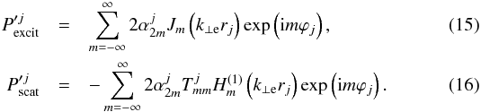Finally, we use the expression of ${\mathit{P}}_{\mathrm{scat}}^{\mathrm{\prime }\mathit{j}}$ into Eq. (10) to arrive at the total net solution in the external plasma, namely 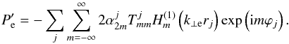${\mathit{P}}_{\mathrm{e}}^{\mathrm{\prime }}\mathrm{=}\mathrm{-}\sum _{\mathit{j}}\sum _{\mathit{m}\mathrm{=}\mathrm{-}\mathrm{\infty }}^{\mathrm{\infty }}\mathrm{2}{\mathit{\alpha }}_{\mathrm{2}\mathit{m}}^{\mathit{j}}{\mathit{T}}_{\mathit{mm}}^{\mathit{j}}{\mathit{H}}_{\mathit{m}}^{\mathrm{\left(}\mathrm{1}\mathrm{\right)}}\mathrm{\left(}{\mathit{k}}_{\mathrm{\perp }\mathrm{e}}{\mathit{r}}_{\mathit{j}}\mathrm{\right)}\exp \mathrm{\left(}\mathrm{i}\mathit{m}{\mathit{\varphi }}_{\mathit{j}}\mathrm{\right)}\mathit{.}$(17)Equations (6) and (17) formally describe the total pressure perturbation in the interior and in the exterior of the tubes, respectively. However, we note that these expressions do not apply in the nonuniform boundary layers. The T-matrix elements, ${\mathit{T}}_{\mathit{mm}}^{\mathit{j}}$, contain the information about how the solutions are connected across the nonuniform boundaries of the tubes.

3.2. T-matrix elements in the thin boundary approximation

At this stage we incorporate the effect of the nonuniform boundary layers. In the nonuniform layer of the jth tube the global wave modes are resonant in the Alfvén continuum at the resonant position, r_j = r_A,j, where the global oscillation frequency matches the local Alfvén frequency. The resonant position, r_A,j, is defined through the resonant condition ${\mathit{\omega }}^{\mathrm{2}}\mathrm{=}{\mathit{k}}_{\mathit{z}}^{\mathrm{2}}{\mathit{v}}_{\mathrm{A}}^{\mathrm{2}}\mathrm{\left(}{\mathit{r}}_{\mathrm{A}\mathit{,j}}\mathrm{\right)}$. We use the TB approximation and restrict ourselves to l_j/R_j ≪ 1. The TB approximation assumes that the jump of the perturbations across the resonant layer is the same as their jump across the whole nonuniform layer. Thus, the connection formulae of the wave perturbations across the resonance are used as jump conditions for the total pressure and the Lagrangian displacement at the boundaries of the tubes. This method and its applications have been reviewed by Goossens et al. (2011). The TB approximation within the formalism of the T-matrix theory has previously been used by Keppens et al. (1994) and Keppens (1995).

General expressions of the connection formulae for the perturbations across the resonant layer can be found in, e.g., Sakurai et al. (1991). In local coordinates, the connection formulae for the total pressure Eulerian pertubation, P′, and the radial component of the Lagrangian displacement, ξ_r, at r_j = r_A,j are $\left[{\mathit{P}}^{\mathrm{\prime }}\right]\mathrm{=}\mathrm{0}\mathit{,} \left[{\mathit{\xi }}_{\mathit{r}}\right]\mathrm{=}\mathrm{-}\mathrm{i}\mathit{\pi }\frac{{\mathit{m}}^{\mathrm{2}}\mathit{/}{\mathit{r}}_{\mathrm{A}\mathit{,j}}^{\mathrm{2}}}{{\left|\mathit{\rho }{\mathrm{\Delta }}_{\mathrm{A}}\right|}_{\mathit{j}}}{\mathit{P}}^{\mathrm{\prime }}\mathit{,}$(18)where [X] = X_e−X_j denotes the jump of the quantity X across the resonant layer and |ρΔ_A|_j is defined as ${\left|\mathit{\rho }{\mathrm{\Delta }}_{\mathrm{A}}\right|}_{\mathit{j}}\mathrm{=}\mathit{\rho }\mathrm{\left(}{\mathit{r}}_{\mathrm{A}\mathit{,j}}\mathrm{\right)}{\left|\frac{\mathrm{d}}{\mathrm{d}{\mathit{r}}_{\mathit{j}}}\mathrm{(}{\mathit{\omega }}^{\mathrm{2}}\mathrm{-}{\mathit{k}}_{\mathit{z}}^{\mathrm{2}}{{\mathit{v}}_{\mathrm{A}}^{\mathrm{2}}}^{\mathrm{)}}\right|}_{{\mathit{r}}_{\mathrm{A}\mathit{,j}}}\mathrm{=}{\mathit{\omega }}^{\mathrm{2}}{\left|\frac{\mathrm{d}\mathit{\rho }}{\mathrm{d}{\mathit{r}}_{\mathit{j}}}\right|}_{{\mathit{r}}_{\mathrm{A}\mathit{,j}}}\mathit{,}$(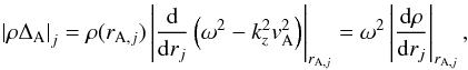19)where we have used the resonant condition ${\mathit{\omega }}^{\mathrm{2}}\mathrm{=}{\mathit{k}}_{\mathit{z}}^{\mathrm{2}}{\mathit{v}}_{\mathrm{A}}^{\mathrm{2}}\mathrm{\left(}{\mathit{r}}_{\mathrm{A}\mathit{,j}}\mathrm{\right)}$. After imposing the jump conditions given in Eq. (18), we obtain both the T-matrix elements and the dispersion relation of the collective modes.

On the one hand, the T-matrix elements are 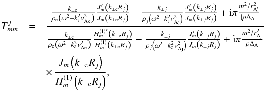$\begin{array}{ccc}{\mathit{T}}_{\mathit{mm}}^{\mathit{j}}& \mathrm{=}& \frac{\frac{{\mathit{k}}_{\mathrm{\perp }\mathrm{e}}}{{\mathit{\rho }}_{\mathrm{e}}\left({\mathit{\omega }}^{\mathrm{2}}\mathrm{-}{\mathit{k}}_{\mathit{z}}^{\mathrm{2}}{\mathit{v}}_{\mathrm{Ae}}^{\mathrm{2}}\right)}\frac{{\mathit{J}}_{\mathit{m}}^{\mathrm{\prime }}\left({\mathit{k}}_{\mathrm{\perp }\mathrm{e}}{\mathit{R}}_{\mathit{j}}\right)}{{\mathit{J}}_{\mathit{m}}\left({\mathit{k}}_{\mathrm{\perp }\mathrm{e}}{\mathit{R}}_{\mathit{j}}\right)}\mathrm{-}\frac{{\mathit{k}}_{\mathrm{\perp }\mathit{j}}}{{\mathit{\rho }}_{\mathit{j}}\left({\mathit{\omega }}^{\mathrm{2}}\mathrm{-}{\mathit{k}}_{\mathit{z}}^{\mathrm{2}}{\mathit{v}}_{\mathrm{Aj}}^{\mathrm{2}}\right)}\frac{{\mathit{J}}_{\mathit{m}}^{\mathrm{\prime }}\left({\mathit{k}}_{\mathrm{\perp }\mathit{j}}{\mathit{R}}_{\mathit{j}}\right)}{{\mathit{J}}_{\mathit{m}}\left({\mathit{k}}_{\mathrm{\perp }\mathit{j}}{\mathit{R}}_{\mathit{j}}\right)}\mathrm{+}\mathrm{i}\mathit{\pi }\frac{{\mathit{m}}^{\mathrm{2}}\mathit{/}{\mathit{r}}_{\mathrm{Aj}}^{\mathrm{2}}}{\mathrm{|}\mathit{\rho }{\mathrm{\Delta }}_{\mathrm{A}}\mathrm{|}}}{\frac{{\mathit{k}}_{\mathrm{\perp }\mathrm{e}}}{{\mathit{\rho }}_{\mathrm{e}}\left({\mathit{\omega }}^{\mathrm{2}}\mathrm{-}{\mathit{k}}_{\mathit{z}}^{\mathrm{2}}{\mathit{v}}_{\mathrm{Ae}}^{\mathrm{2}}\right)}\frac{{{\mathit{H}}_{\mathit{m}}^{\mathrm{\left(}\mathrm{1}\mathrm{\right)}}}^{\mathrm{\prime }}\left({\mathit{k}}_{\mathrm{\perp }\mathrm{e}}{\mathit{R}}_{\mathit{j}}\right)}{{\mathit{H}}_{\mathit{m}}^{\mathrm{\left(}\mathrm{1}\mathrm{\right)}}\left({\mathit{k}}_{\mathrm{\perp }\mathrm{e}}{\mathit{R}}_{\mathit{j}}\right)}\mathrm{-}\frac{{\mathit{k}}_{\mathrm{\perp }\mathit{j}}}{{\mathit{\rho }}_{\mathit{j}}\left({\mathit{\omega }}^{\mathrm{2}}\mathrm{-}{\mathit{k}}_{\mathit{z}}^{\mathrm{2}}{\mathit{v}}_{\mathrm{Aj}}^{\mathrm{2}}\right)}\frac{{\mathit{J}}_{\mathit{m}}^{\mathrm{\prime }}\left({\mathit{k}}_{\mathrm{\perp }\mathit{j}}{\mathit{R}}_{\mathit{j}}\right)}{{\mathit{J}}_{\mathit{m}}\left({\mathit{k}}_{\mathrm{\perp }\mathit{j}}{\mathit{R}}_{\mathit{j}}\right)}\mathrm{+}\mathrm{i}\mathit{\pi }\frac{{\mathit{m}}^{\mathrm{2}}\mathit{/}{\mathit{r}}_{\mathrm{Aj}}^{\mathrm{2}}}{\mathrm{|}\mathit{\rho }{\mathrm{\Delta }}_{\mathrm{A}}\mathrm{|}}}\\ & & \end{array}$(20)where the prime ′ denotes the derivative of the Bessel or Hankel function with respect to its argument. In the absence of resonant damping, Eq. (20) consistently reverts to Eq. (17) of Luna et al. (2009).

On the other hand, the constants ${\mathit{\alpha }}_{\mathrm{2}\mathit{m}}^{\mathit{j}}$ satisfy an algebraic system of equations, namely 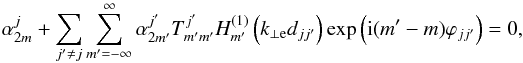${\mathit{\alpha }}_{\mathrm{2}\mathit{m}}^{\mathit{j}}\mathrm{+}\sum _{{\mathit{j}}^{\mathrm{\prime }}\ne \mathit{j}}\sum _{{\mathit{m}}^{\mathrm{\prime }}\mathrm{=}\mathrm{-}\mathrm{\infty }}^{\mathrm{\infty }}{\mathit{\alpha }}_{\mathrm{2}{\mathit{m}}^{\mathrm{\prime }}}^{{\mathit{j}}^{\mathrm{\prime }}}{\mathit{T}}_{{\mathit{m}}^{\mathrm{\prime }}{\mathit{m}}^{\mathrm{\prime }}}^{{\mathit{j}}^{\mathrm{\prime }}}{\mathit{H}}_{{\mathit{m}}^{\mathrm{\prime }}}^{\mathrm{\left(}\mathrm{1}\mathrm{\right)}}\mathrm{\left(}{\mathit{k}}_{\mathrm{\perp }\mathrm{e}}{\mathit{d}}_{\mathit{j}{\mathit{j}}^{\mathrm{\prime }}}\mathrm{\right)}\exp \mathrm{\left(}\mathrm{i}\mathrm{\right(}{\mathit{m}}^{\mathrm{\prime }}\mathrm{-}\mathit{m}\mathrm{\left)}{\mathit{\varphi }}_{\mathit{j}{\mathit{j}}^{\mathrm{\prime }}}\mathrm{\right)}\mathrm{=}\mathrm{0}\mathit{,}$(21)for −∞ <m< ∞, where ϕ_jj′ is the angle formed by the vector positions of the centers of the two tubes with respect to the global reference frame. Equation (21) is a system with an infinite number of algebraic equations. The condition that there is a nontrivial solution, i.e., the determinant formed by the coefficients set equal to zero, provides us with the dispersion relation (see details in Luna et al. 2009, 2010). The solution of the dispersion relation is the complex frequency of the damped collective quasi-mode. The imaginary part of the frequency is the resonant damping rate. In the case of Luna et al. (2009, 2010), the solution frequency was real because of the absence of resonant damping.

The dispersion relation is a complicated expression and has to be solved by numerical methods. For practical computational purposes, in Eq. (21) the indices m and m′ must be truncated into a finite number. The truncation term must be large enough to avoid inaccuracy of the solutions. Then, the dispersion relation can be solved using standard numerical routines to find the roots of transcendental equations.

4. Application to damped oscillations of two loops

We note that the T-matrix theory described in the previous Section is valid for an arbitrary number of loops. Here we apply that method to investigate damped transverse oscillations in a loop system composed of two magnetic tubes alone. First we derive approximate expressions of the period and damping time in the case of two identical thin tubes. Later, we consider two tubes with different properties and arbitrary radii and perform a numerical study.

4.1. Approximate solutions for two identical thin tubes

We consider the paradigmatic case of two tubes with identical properties. We denote by ρ_i, R, and l the internal density, the radius, and the thickness of the boundary layer of both tubes, respectively. The external density remains ρ_e. The distance between the centers of the two tubes is d.

To obtain an approximate dispersion relation for kink-like modes we assume that the contribution from the azimuthal wavenumbers m = ± 1 to the collective oscillation is much more important than the contributions from other values of m. Thus, we take m,m′ = ± 1 in Eq. (21) and roughly neglect the other terms. As pointed out by Luna et al. (2009), the coupling between the different values of m gets stronger as the separation between the cylinders decreases. In terms of the parameters of the model, this means that our approximation applies to the case of large separations, i.e., R/d ≪ 1.

The system defined in Eq. (21) now becomes an algebraic system of four equations for the unknowns ${\mathit{\alpha }}_{\mathrm{2}\mathit{,}\mathrm{-}\mathrm{1}}^{\mathrm{1}}$, ${\mathit{\alpha }}_{\mathrm{2}\mathit{,}\mathrm{1}}^{\mathrm{1}}$, ${\mathit{\alpha }}_{\mathrm{2}\mathit{,}\mathrm{-}\mathrm{1}}^{\mathrm{2}}$, and ${\mathit{\alpha }}_{\mathrm{2}\mathit{,}\mathrm{1}}^{\mathrm{2}}$. We obtain the dispersion relation from the condition that there is a nontrivial solution of the system, namely 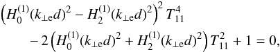$\begin{array}{ccc}& & {\mathrm{(}{\mathit{H}}_{\mathrm{0}}^{\mathrm{\left(}\mathrm{1}\mathrm{\right)}}\mathrm{(}{\mathit{k}}_{\mathrm{\perp }\mathrm{e}}\mathit{d}{\mathrm{)}}^{\mathrm{2}}\mathrm{-}{\mathit{H}}_{\mathrm{2}}^{\mathrm{\left(}\mathrm{1}\mathrm{\right)}}\mathrm{(}{\mathit{k}}_{\mathrm{\perp }\mathrm{e}}\mathit{d}{\mathrm{)}}^{\mathrm{2}}\mathrm{)}}^{\mathrm{2}}{\mathit{T}}_{\mathrm{11}}^{\mathrm{4}}\\ & & \end{array}$(22)where we used the property that T₁₁ = T_{− 1−1} according to the symmetry relations of the Bessel and Hankel functions (see Abramowitz & Stegun 1972). Equation (22) is an equation for ω, which is enclosed in the definitions of T₁₁ and k_{⊥ e}. To go further analytically, we perform a series expansion of the Hankel functions for small arguments and retain the first term alone. This would be approximately valid for thin tubes. After some algebraic manipulations, Eq. (22) can be recast as 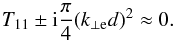${\mathit{T}}_{\mathrm{11}}\mathrm{\pm }\mathrm{i}\frac{\mathit{\pi }}{\mathrm{4}}\mathrm{(}{\mathit{k}}_{\mathrm{\perp }\mathrm{e}}\mathit{d}{\mathrm{)}}^{\mathrm{2}}\mathrm{\approx }\mathrm{0.}$(23)Now, we look for a simplified expression of T₁₁. We use the TT approximation, i.e., R/L ≪ 1. In Eq. (20) we perform an asymptotic expansion of the Bessel and Hankel functions for small arguments. Equation (20) becomes 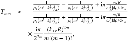$\begin{array}{ccc}{\mathit{T}}_{\mathit{mm}}& \mathrm{\approx }& \mathrm{-}\frac{\frac{\mathrm{1}}{{\mathit{\rho }}_{\mathrm{e}}\left({\mathit{\omega }}^{\mathrm{2}}\mathrm{-}{\mathit{k}}_{\mathit{z}}^{\mathrm{2}}{\mathit{v}}_{\mathrm{Ae}}^{\mathrm{2}}\right)}\mathrm{-}\frac{\mathrm{1}}{{\mathit{\rho }}_{\mathrm{i}}\left({\mathit{\omega }}^{\mathrm{2}}\mathrm{-}{\mathit{k}}_{\mathit{z}}^{\mathrm{2}}{\mathit{v}}_{\mathrm{Ai}}^{\mathrm{2}}\right)}\mathrm{+}\mathrm{i}\mathit{\pi }\frac{\mathit{m}\mathit{/}\mathit{R}}{{\mathit{\omega }}_{\mathrm{R}}^{\mathrm{2}}{\left|\mathrm{d}\mathit{\rho }\mathit{/}\mathrm{d}\mathit{r}\right|}_{\mathit{R}}}}{\frac{\mathrm{1}}{{\mathit{\rho }}_{\mathrm{e}}\left({\mathit{\omega }}^{\mathrm{2}}\mathrm{-}{\mathit{k}}_{\mathit{z}}^{\mathrm{2}}{\mathit{v}}_{\mathrm{Ae}}^{\mathrm{2}}\right)}\mathrm{+}\frac{\mathrm{1}}{{\mathit{\rho }}_{\mathrm{i}}\left({\mathit{\omega }}^{\mathrm{2}}\mathrm{-}{\mathit{k}}_{\mathit{z}}^{\mathrm{2}}{\mathit{v}}_{\mathrm{Ai}}^{\mathrm{2}}\right)}\mathrm{-}\mathrm{i}\mathit{\pi }\frac{\mathit{m}\mathit{/}\mathit{R}}{{\mathit{\omega }}_{\mathrm{R}}^{\mathrm{2}}{\left|\mathrm{d}\mathit{\rho }\mathit{/}\mathrm{d}\mathit{r}\right|}_{\mathit{R}}}}\\ & & \end{array}$(24)where we also assumed r_A ≈ R for simplicity. We take m = 1, substitute Eq. (24) into Eq. (23), and arrive at the following expression, 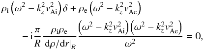$\begin{array}{ccc}& & {\mathit{\rho }}_{\mathrm{i}}\mathrm{(}{\mathit{\omega }}^{\mathrm{2}}\mathrm{-}{\mathit{k}}_{\mathit{z}}^{\mathrm{2}}{{\mathit{v}}_{\mathrm{Ai}}^{\mathrm{2}}}^{\mathrm{)}}\mathit{\delta }\mathrm{+}{\mathit{\rho }}_{\mathrm{e}}\mathrm{(}{\mathit{\omega }}^{\mathrm{2}}\mathrm{-}{\mathit{k}}_{\mathit{z}}^{\mathrm{2}}{{\mathit{v}}_{\mathrm{Ae}}^{\mathrm{2}}}^{\mathrm{)}}\\ & & \end{array}$(25)where the parameter δ is defined as 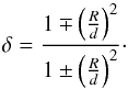$\mathit{\delta }\mathrm{=}\frac{\mathrm{1}\mathrm{\mp }{\mathrm{(}{\frac{\mathit{R}}{\mathit{d}}}^{\mathrm{)}}}^{\mathrm{2}}}{\mathrm{1}\mathrm{\pm }{\mathrm{(}{\frac{\mathit{R}}{\mathit{d}}}^{\mathrm{)}}}^{\mathrm{2}}}\mathrm{·}$(26)Equation (25) is the dispersion relation for resonantly damped kink modes of two identical tubes in the TT and TB approximations and for large separations. In the limit that the tubes are far from each other, R/d → 0 and so δ → 1. Then, Eq. (25) consistently reverts to the dispersion relation of resonant kink modes in an isolated thin tube (e.g., Goossens et al. 1992).

4.1.1. Frequency of the oscillations

First we neglect the presence of the nonuniform boundary layers and study undamped oscillations. We drop the last term on the left-hand side of Eq. (25) and the dispersion relation simplifies to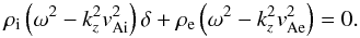${\mathit{\rho }}_{\mathrm{i}}\mathrm{(}{\mathit{\omega }}^{\mathrm{2}}\mathrm{-}{\mathit{k}}_{\mathit{z}}^{\mathrm{2}}{{\mathit{v}}_{\mathrm{Ai}}^{\mathrm{2}}}^{\mathrm{)}}\mathit{\delta }\mathrm{+}{\mathit{\rho }}_{\mathrm{e}}\mathrm{(}{\mathit{\omega }}^{\mathrm{2}}\mathrm{-}{\mathit{k}}_{\mathit{z}}^{\mathrm{2}}{{\mathit{v}}_{\mathrm{Ae}}^{\mathrm{2}}}^{\mathrm{)}}\mathrm{=}\mathrm{0.}$(27)The exact solution is 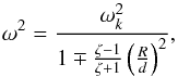${\mathit{\omega }}^{\mathrm{2}}\mathrm{=}\frac{{\mathit{\omega }}_{\mathit{k}}^{\mathrm{2}}}{\mathrm{1}\mathrm{\mp }\frac{\mathit{\zeta }\mathrm{-}\mathrm{1}}{\mathit{\zeta }\mathrm{+}\mathrm{1}}{\mathrm{(}{\frac{\mathit{R}}{\mathit{d}}}^{\mathrm{)}}}^{\mathrm{2}}}\mathit{,}$(28)where ζ = ρ_i/ρ_e is the density contrast and ω_k is the frequency of the kink mode in an individual thin tube (Edwin & Roberts 1983), namely 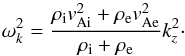${\mathit{\omega }}_{\mathit{k}}^{\mathrm{2}}\mathrm{=}\frac{{\mathit{\rho }}_{\mathrm{i}}{\mathit{v}}_{\mathrm{Ai}}^{\mathrm{2}}\mathrm{+}{\mathit{\rho }}_{\mathrm{e}}{\mathit{v}}_{\mathrm{Ae}}^{\mathrm{2}}}{{\mathit{\rho }}_{\mathrm{i}}\mathrm{+}{\mathit{\rho }}_{\mathrm{e}}}{\mathit{k}}_{\mathit{z}}^{\mathrm{2}}\mathrm{·}$(29)Equation (28) can be compared to Eq. (51) of Van Doorsselaere et al. (2008). Both expressions agree if the parameter E of Van Doorsselaere et al. (2008) is approximated as $\mathit{E}\mathrm{=}\exp {}^{\mathrm{[}}\mathrm{-}\mathrm{2}\mathrm{arccosh}\mathrm{(}\frac{\mathit{d}}{\mathrm{2}\mathit{R}}{\mathrm{\left)}}^{\mathrm{\right]}}\mathrm{\approx }{{}^{\mathrm{\right(}}\frac{\mathit{R}}{\mathit{d}}^{\mathrm{\left)}}}^{\mathrm{2}}$, which is valid for R/d ≪ 1. In agreement with Van Doorsselaere et al. (2008), in the TT approximation we obtain two kink-like solutions corresponding to the + and − signs in Eq. (28). As explained by Luna et al. (2009), there are actually four kink-like modes beyond the TT approximation. For arbitrary radii, the low-frequency solution (that with the + sign in Eq. (28)) splits in the S_x and A_y modes of Luna et al. (2009), while the high-frequency solution (that with the − sign in Eq. (28)) becomes their S_y and A_x solutions.

From Eq. (28) we compute the period of the oscillations, P = 2π/ω, as 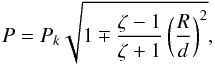$\mathit{P}\mathrm{=}{\mathit{P}}_{\mathit{k}}\sqrt{\mathrm{1}\mathrm{\mp }\frac{\mathit{\zeta }\mathrm{-}\mathrm{1}}{\mathit{\zeta }\mathrm{+}\mathrm{1}}{\left(\frac{\mathit{R}}{\mathit{d}}\right)}^{\mathrm{2}}}\mathit{,}$(30)with P_k = 2π/ω_k the period of the kink mode of an isolated tube. For large separations the tubes feel little interaction. Then, the periods of the two solutions consistently tend to that of the kink mode of an isolated tube.

4.1.2. Damping rate

Here we incorporate the effect of resonant damping and consider the full expression of the dispersion relation (Eq. (25)). To obtain an approximate expression of the damping rate, we substitute ω = ω_R + iω_I in Eq. (25) and assume weak damping, i.e., | ω_I | ≪ | ω_R |. Then, we are allowed to neglect terms of order ${\mathit{\omega }}_{\mathrm{I}}^{\mathrm{2}}$ and higher orders. After some algebraic maniputations (not given here for the sake of simplicity) we arrive at an expression for the ratio ω_I/ω_R, namely 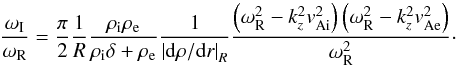$\frac{{\mathit{\omega }}_{\mathrm{I}}}{{\mathit{\omega }}_{\mathrm{R}}}\mathrm{=}\frac{\mathit{\pi }}{\mathrm{2}}\frac{\mathrm{1}}{\mathit{R}}\frac{{\mathit{\rho }}_{\mathrm{i}}{\mathit{\rho }}_{\mathrm{e}}}{{\mathit{\rho }}_{\mathrm{i}}\mathit{\delta }\mathrm{+}{\mathit{\rho }}_{\mathrm{e}}}\frac{\mathrm{1}}{{\left|\mathrm{d}\mathit{\rho }\mathit{/}\mathrm{d}\mathit{r}\right|}_{\mathit{R}}}\frac{\mathrm{(}{\mathit{\omega }}_{\mathrm{R}}^{\mathrm{2}}\mathrm{-}{\mathit{k}}_{\mathit{z}}^{\mathrm{2}}{{\mathit{v}}_{\mathrm{Ai}}^{\mathrm{2}}}^{\mathrm{)}}\mathrm{(}{\mathit{\omega }}_{\mathrm{R}}^{\mathrm{2}}\mathrm{-}{\mathit{k}}_{\mathit{z}}^{\mathrm{2}}{{\mathit{v}}_{\mathrm{Ae}}^{\mathrm{2}}}^{\mathrm{)}}}{{\mathit{\omega }}_{\mathrm{R}}^{\mathrm{2}}}\mathrm{·}$(31)To simplify Eq. (31) we consider a smooth monotonic profile for the density in the nonuniform boundaries so that we can express the derivative of the density profile as 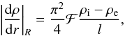${\left|\frac{\mathrm{d}\mathit{\rho }}{\mathrm{d}\mathit{r}}\right|}_{\mathit{R}}\mathrm{=}\frac{{\mathit{\pi }}^{\mathrm{2}}}{\mathrm{4}}\mathrm{ℱ}\frac{{\mathit{\rho }}_{\mathrm{i}}\mathrm{-}{\mathit{\rho }}_{\mathrm{e}}}{\mathit{l}}\mathit{,}$(32)with ℱ a factor that depends on the form of the profile. For instance, ℱ = 4 /π² for a linear profile and ℱ = 2 /π for a sinusoidal profile. In addition, we approximate ω_R by the value of the frequency in the undamped case (Eq. (28)) and substitute the expression of δ (Eq. (26)) to arrive at $\frac{{\mathit{\omega }}_{\mathrm{I}}}{{\mathit{\omega }}_{\mathrm{R}}}\mathrm{\approx }\mathrm{-}\frac{\mathrm{1}}{\mathrm{2}\mathit{\pi }}\frac{\mathrm{1}}{\mathrm{ℱ}}\frac{\mathit{l}}{\mathit{R}}\frac{\mathit{\zeta }\mathrm{-}\mathrm{1}}{\mathit{\zeta }\mathrm{+}\mathrm{1}}\frac{\mathrm{1}\mathrm{\pm }{\mathrm{(}{\frac{\mathit{R}}{\mathit{d}}}^{\mathrm{)}}}^{\mathrm{2}}}{\mathrm{1}\mathrm{\mp }\frac{\mathit{\zeta }\mathrm{-}\mathrm{1}}{\mathit{\zeta }\mathrm{+}\mathrm{1}}{\mathrm{(}{\frac{\mathit{R}}{\mathit{d}}}^{\mathrm{)}}}^{\mathrm{2}}}\left[\mathrm{1}\mathrm{-}{\left(\frac{\mathit{R}}{\mathit{d}}\right)}^{\mathrm{4}}\right]\mathrm{·}$(33)For a linear density profile, Eq. (33) becomes Eq. (86) of Robertson & Ruderman (2011) if the approximation $\exp \mathrm{[}\mathrm{-}\mathrm{2}\mathrm{arccosh}\mathrm{(}\frac{\mathit{d}}{\mathrm{2}\mathit{R}}\mathrm{\left)}\mathrm{\right]}\mathrm{\approx }{{}^{\mathrm{\right(}}\frac{\mathit{R}}{\mathit{d}}^{\mathrm{\left)}}}^{\mathrm{2}}$ valid for R/d ≪ 1 is again performed in their expression.

Now, we define the damping time as τ_D = 1/ | ω_I | and use Eq. (33) to obtain the expression for the ratio τ_D/P. By keeping terms up to (R/d)², the expression for the damping ratio is$\frac{{\mathit{\tau }}_{\mathrm{D}}}{\mathit{P}}\mathrm{\approx }{\left(\frac{{\mathit{\tau }}_{\mathrm{D}}}{\mathit{P}}\right)}_{\mathrm{k}}\left[\mathrm{1}\mathrm{\mp }\frac{\mathrm{2}\mathit{\zeta }}{\mathit{\zeta }\mathrm{+}\mathrm{1}}{\left(\frac{\mathit{R}}{\mathit{d}}\right)}^{\mathrm{2}}\right]\mathit{,}$(34)where ${\left(\frac{{\mathit{\tau }}_{\mathrm{D}}}{\mathit{P}}\right)}_{\mathrm{k}}\mathrm{=}\mathrm{ℱ}\frac{\mathit{R}}{\mathit{l}}\frac{\mathit{\zeta }\mathrm{+}\mathrm{1}}{\mathit{\zeta }\mathrm{-}\mathrm{1}}\mathit{,}$(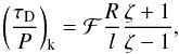35)is the damping ratio of the individual kink mode (see, e.g., Ruderman & Roberts 2002; Goossens et al. 2002). As for individual kink modes, the damping ratio of collective modes is inversely proportional to the thickness of the nonuniform layer. Equation (34) shows that the solution with the + sign is more efficiently damped by resonant absorption than the solution with the − sign. This difference in the damping rates of the two modes qualitatively agrees with the results of Robertson & Ruderman (2011).

4.2. Numerical study

Here we perform a numerical study beyond the approximate limits studied before. To do so, we consider the full dispersion relation obtained from Eq. (21) by using the general expression of the T-matrix elements (Eq. (20)). The truncated dispersion relation is then numerically solved. Convergence tests of the results have been performed to make sure that the truncation value of the azimuthal series is large enough for the error on the solutions to be negligible. In short, we found that for kink-like modes the truncation value, namely m_t, has no important effect unless m_t< 5 and the two loops are next to each other (d/R ≈ 2). When m_t> 5 and/or the loops are far from each other, we essentially obtain that the results are independent of m_t. We have used m_t = 30 in all computations given here, which reduces the error and ensures the excellent converge of the solutions even when d/R ≈ 2.

The numerical method follows a two-step procedure. First, we solve the dispersion relation in the absence of nonuniform boundary layers. In that case, the solution is a real frequency that corresponds to an approximation to ω_R. This approximate value of ω_R is used to compute the resonance positions and the derivative of the density profile at the resonances. We assume sinusoidal density profiles in the nonuniform boundary layers. Then, we use these parameters to solve the complete dispersion relation, which now includes the effect of resonant damping. The frequency obtained from the second run is complex, so that it provides us with a more accurate value of ω_R and also gives us the value of ω_I.

4.2.1. Identical loops

We initially study the case of two identical tubes. We set the Cartesian coordinates system so that the xy-plane is perpendicular to the axes of the loops. In that plane, the centers of the two loops are located on the x-axis. We use the notation introduced by Luna et al. (2008) to denote the four kink-like modes present in a two-loop configuration. The modes are labeled as S_x, A_x, S_y, and A_y, where S and A denote symmetric or anti-symmetric motions of the two loops, respectively, and the subscripts x and y indicate the main direction of polarization of the oscillations in the coordinates system defined above. The eigenfunctions of these four modes in the case of loops without nonuniform boundary layers can be found in Fig. 2 of Luna et al. (2008).

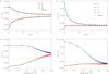Fig. 2 Numerical results in the case of two identical coronal loops. a) Dependence of ωR/ωA,e on d/R, where ωA,e = kzvA,e is the external Alfvén frequency. b) Dependence of |ωI| /ωR on d/R. The meaning of the various lines is indicated within the panels. The dashed lines correspond to the analytic approximations in the limit d/R ≫ 1 (Eqs. (28) and (33)). We have used ζ = 5, L/R = 100, and l/R = 0.2. Panels c) and d) show the same results as panels a) and b), respectively, but as functions of log 10(d/R−2).

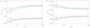Fig. 3 Numerical results in the case of two identical coronal loops. a) Dependence of ωR/ωA,e on L/R, where ωA,e = kzvA,e is the external Alfvén frequency. b) Dependence of |ωI| /ωR on L/R. The meaning of the various lines is indicated within the figure. We have used ζ = 5, l/R = 0.2, and d/R = 2.5. We note that the horizontal axes of both panels are in logarithmic scale.

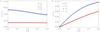Fig. 4 Numerical results in the case of two identical coronal loops. a) Dependence of ωR/ωA,e on l/R, where ωA,e = kzvA,e is the external Alfvén frequency. b) Dependence of |ωI| /ωR on l/R. The meaning of the various lines is indicated within the figure. We have used ζ = 5, L/R = 100, and d/R = 2.5.

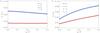Fig. 5 Numerical results in the case of two non-identical coronal loops with R1 = R2 = R. a) Dependence of ωR/ωA,e on l2/R, where ωA,e = kzvA,e is the external Alfvén frequency. b) Dependence of |ωI| /ωR on l2/R. The meaning of the various lines is indicated within the figure. We have used ζ1 = ζ2 = 5, L/R = 100, l1/R = 0.2 and d/R = 2.5.

Figure 2 shows the dependence of ω_R and the ratio |ω_I| /ω_R on the separation between loops, d/R, for a particular set of parameters given in the caption of the figure. We note that the curves corresponding to the S_x and A_y modes, and those of the A_x and S_y modes, are almost superimposed because we are in the TT regime (we used L/R = 100). Concerning the behavior of ω_R, the frequencies of the four solutions tend to the kink frequency of an isolated loop in the limit d/R ≫ 1. Conversely, the smaller the separation between loops, the more important the splitting of the collective frequencies with respect to the kink frequency of an isolated loop. Figure 2a can be compared to Fig. 3 of Luna et al. (2008) and with Fig. 4 of Van Doorsselaere et al. (2008). However, unlike in those previous works we note that in our case the frequencies of the high-frequency solutions (A_x and S_y) do not tend to the external Alfvén frequency when d/R → 2. The reason for this difference is probably that the A_x and S_y modes are strongly damped when d/R → 2, and this has some impact on the real part of the frequency as well.

On the other hand, Fig. 2b shows that the high-frequency modes (A_x and S_y) are more efficiently damped by resonant absorption than the low-frequency modes (S_x and A_y). This result agrees with that of Robertson & Ruderman (2011) for large separations. However, the behavior of |ω_I| /ω_R obtained here for small separations is dramatically different from that of Robertson & Ruderman (2011). They found that the oscillations become undamped in the limit d/R → 2, while we find that the modes remain damped. Although the analysis of Robertson & Ruderman (2011) is mathematically correct, we find no physical reason for which the oscillations should be undamped when the loops are close to each other. Our computations show that the damping of the low-frequency modes (S_x and A_y) is roughly independent on d/R, whereas the damping of the high-frequency modes (A_x and S_y) gets stronger as the separation between loops is reduced. As pointed out by Robertson & Ruderman (2011) and Gijsen & Van Doorsselaere (2014), the physical significance of the results obtained with bycilindrical coordinates should be treated with caution when the separation between the tubes is small.

Panels c and d of Fig. 2 show the same results as panels a and b, respectively, but now log ₁₀⁽l/R−2⁾ is used in the horizontal axes. These additional graphs are included to show in more detail the behavior of the solutions obtained with the T-matrix method for small separations between tubes.

We have overplotted in Fig. 2 the analytic approximations of ω_R and |ω_I| /ω_R given in Eqs. (28) and (33). These approximations were derived in the limit d/R ≫ 1 and reasonably agree with the numerical solutions when d/R ≳ 3. As expected, the approximations do not work well for small separations. The analytic approximations were derived considering the contributions from m = ± 1 alone, but the contribution of high m’s to the full solution is important for small separation between loops (see Luna et al. 2009).

Figure 3 shows the dependence of the solutions on L/R. This figure is included to show that the almost degenerate couples S_x–A_y and A_x–S_y split into four different solutions for small values of L/R beyond the TT regime. We point out, however, that the impact of the value of L/R on the solutions is not relevant when realistic values of this parameter are considered. The TT limit used by Robertson & Ruderman (2011) and Gijsen & Van Doorsselaere (2014) is therefore adequate.

Now we plot in Fig. 4 the dependence of ω_R and |ω_I| /ω_R on the nonuniform layer thickness, l/R. We consider a small separation, namely d/R = 2.5, and the remaining parameters are the same as in Fig. 2. Consistently, when l/R = 0 the modes are undamped. The real part of the frequency of the low-frequency modes is almost independent of l/R, while their |ω_I| /ω_R is roughly linear with l/R. Conversely, the real part of the frequency of the low-frequency modes decreases when l/R increases, and their |ω_I| /ω_R is only linear with l/R for small values of this parameter. As discussed before, the behavior of the low-frequency modes (S_x and A_y) is similar to that of the kink mode of an isolated loop. However, the high-frequency modes (A_x and S_y) seem to be more affected by the interaction between loops and show a somewhat different behavior when l/R increases. We note that because of the TB approximation we are restricted to consider small values of l/R.

It is useful to relate the present results with those of Arregui et al. (2007, 2008), who studied the damping of transverse oscillations of two nonuniform slabs. They found that the ratio |ω_I| /ω_R corresponding to the symmetric kink mode of the two slabs is weakly dependent of the separation between the two slabs (see Arregui et al. 2007, their Fig. 4). In turn, Arregui et al. (2008) found that the anti-symmetric kink mode of the two slabs is more efficiently damped than the symmetric kink mode (see their Fig. 6). The symmetric and anti-symmetric kink modes of two slabs would be equivalent to the S_x and A_x modes of two cylinders. Thus, our results in cylindrical geometry are consistent with previous findings in Cartesian geometry.

It is also convenient to consider the physical arguments of Arregui et al. (2007, 2008) to explain why the high-frequency modes damp more efficiently than the low-frequency modes. Arregui et al. (2007, 2008) related the efficiency of the damping with the magnitude of the total pressure perturbation within the resonant layers. According to Andries et al. (2000), the efficiency of the resonant coupling between the global transverse mode and the Alfvén continuum modes is proportional to the total pressure perturbation squared. Soler (2010) plotted the square of the total pressure perturbation corresponding to the S_x and A_x modes (see his Figs. 9.7 and 9.8) and found that, when the quantities are normalized, the perturbation of the A_x mode reaches a larger value in the resonant layers than that of the S_x solution. This result qualitatively explains why resonant damping is more efficient for the A_x mode than for the S_x mode. Equivalently, a similar reasoning help us understand the different attenuation of the S_y and A_y modes. Nevertheless, a more robust study of the process of resonant absorption in two-dimensional configurations would be needed for a complete understanding of the different damping rates (see Russell & Wright 2010).

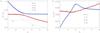Fig. 6 Numerical results in the case of two non-identical coronal loops with R1 = R2 = R. a) Dependence of ωR/ωA,e on ζ1, where ωA,e = kzvA,e is the external Alfvén frequency. b) Dependence of |ωI| /ωR on ζ1. The dotted lines correspond to the Alfvén frequencies of the two loops, and the meaning of the remaining lines is indicated within the figure. We have used ζ2 = 3, L/R = 100, l1/R = l2/R = 0.2 and d/R = 3.

4.2.2. Non-identical loops

Here we consider two loops with different properties and compare our results to those of Gijsen & Van Doorsselaere (2014). We use subscripts 1 and 2 to refer to the two different loops. For simplicity, we take R₁ = R₂ = R and L/R = 100 in all following computations.

First, we assume the same density contrast in the two loops, namely ζ₁ = ζ₂ = 5, and vary l₂/R while l₁/R is kept fixed to l₁/R = 0.2. These results are shown in Fig. 5 and can be compared to those already presented in Fig. 4 in the case of l₁ = l₂. Importantly, we find that the collective oscillations remain damped when l₂/R = 0. Although this is a rather particular situation, the results have interesting implications. When l₂/R = 0 resonant absorption only occurs in the boundary layer of loop #1. However, this is enough for the collective oscillations of the two loops to be efficiently damped. We note that in the study by Gijsen & Van Doorsselaere (2014) the thicknesses of the nonuniform layers are linked to the coordinate system.

Now we consider the case of two loops with different density contrasts. We fix ζ₂ = 3 and compute the solutions as functions of ζ₁. These results are given in Fig. 6, where the remaining parameters used in the computations are specified in the caption. For consistency, we keep the same notation as before to denote the various modes according to the ordering of their frequencies, although they do not represent truly collective oscillations if ζ₁ ≠ ζ₂ (Luna et al. 2009). Figure 6 can be compared to Fig. 6 of Gijsen & Van Doorsselaere (2014). To make a proper comparison, we note that Gijsen & Van Doorsselaere (2014) plotted the signed damping ratio, while here we plot the absolute value.

For the real part of the frequency (Fig. 6a), we find the same results as Luna et al. (2009). When ζ₁<ζ₂, the high-frequency modes are associated with loop #1 alone, whereas the low-frequency modes represent individual oscillations of loop #2. The opposite happens when ζ₁>ζ₂. Conversely, when ζ₁ ≈ ζ₂ the four modes approach and interact in the form of what is known as an avoided crossing. Only in that case do the modes represent truly collective oscillations (Luna et al. 2009).

Figure 6a also shows that the high-frequency modes are always within the Alfvén continua of the two loops, i.e., the frequencies of the A_x and S_y modes are always larger than ω_A,1 and ω_A,2 and smaller than ω_A,e. This is true except in the limit ζ₁ → 1, where the frequencies of the A_x and S_y modes tend to ω_A,e. On the contrary, the low-frequency S_x and A_y modes are below the Alfvén continuum of loop #1 when ζ₁ ≲ 2 and below the Alfvén continuum of loop #2 when ζ₁ ≳ 5. This result may have implications for the damping by resonant absorption.

Figure 6b shows the damping ratio of the modes as a function of ζ₁. The result for the high-frequency modes can be understood as follows. When ζ₁ → 1 the frequencies of the high-frequency modes tend to ω_A,e and, as a consequence, these modes become undamped in that limit. When 1 <ζ₁<ζ₂, the damping ratio increases when ζ₁ increases. When 1 <ζ₁<ζ₂ the high-frequency modes represent individual oscillations of loop #1. Then, the damping ratio reaches a maximum when ζ₁ ≈ ζ₂. When ζ₁>ζ₂ the damping ratio saturates to a constant value because the high-frequency modes represent now individual oscillations of loop #2, and the value of ζ₂ is fixed in the computations. The behavior of the damping of the high-frequency modes agrees with that plotted by Gijsen & Van Doorsselaere (2014) in their Fig. 6.

The overall behavior of the damping ratio of the low-frequency modes presented in Fig. 6b also agrees with Gijsen & Van Doorsselaere (2014). The damping ratio of the low-frequency modes is roughly constant when ζ₁<ζ₂ and increases when ζ₁>ζ₂. The low-frequency modes are below the Alfvén continuum of loop #1 when ζ₁ ≲ 2 and below the Alfvén continuum of loop #2 when ζ₁ ≳ 5, but this has no important impact on the damping. Again, these results can be understood by considering that the low-frequency modes are associated with loop #2 when ζ₁<ζ₂, while they are associated with loop #1 when ζ₁>ζ₂.

The low-frequency modes computed here do not show the pronounced minimum of the damping rate seen in the solution plotted by Gijsen & Van Doorsselaere (2014) when ζ₁ ≈ ζ₂. There are several effects that may explain this difference. The most obvious one is the different geometry considered in Gijsen & Van Doorsselaere (2014) and here. Another possible explanation is that the density profile in the nonuniform layers used by Gijsen & Van Doorsselaere (2014) is different from that used here. A linear density profile is used in Gijsen & Van Doorsselaere (2014), so that the derivative of density at the resonance position is independent of the frequency of the mode. Here we use a sinusoidal profile and take into account that the position of the resonance and the value of the derivative of density at the resonance position are functions of the mode frequency.

In Fig. 6b, the damping rate of the low-frequency modes shows a small bump around ζ₁ ≈ 2, when the real part of the frequency approximately crosses the internal Alfvén frequency of loop #1. The reason for this bump is that the low-frequency modes intersect with and avoid-cross the fluting modes that cluster toward the internal Alfvén frequency. This bump is absent from Fig. 6 of Gijsen & Van Doorsselaere (2014) probably because coupling between kink and fluting modes is not described in the TT approximation.

5. Concluding remarks

In this paper we have extended the analytic T-matrix theory of scattering of Luna et al. (2009, 2010) to investigate resonantly damped oscillations of an arbitrary configuration of parallel cylindrical coronal loops. After presenting the general theory, we have performed a specific application in the case of two loops. This work is partially based on unpublished results included in Soler (2010), where collective damped oscillations of prominence threads were studied.

We have compared our results to those of the papers by Robertson & Ruderman (2011) and Gijsen & Van Doorsselaere (2014). They investigated the damping of collective oscillations of two loops in the TT approximation and used a method based on bicylindrical coordinates. In general, the results of Robertson & Ruderman (2011) and Gijsen & Van Doorsselaere (2014) are in good agreement with the present results, specially when the separation between loops is large. However, when the separation between the loops is small, i.e., for separations of a few radii, the results of those previous works show important differences with the present findings. For instance, Robertson & Ruderman (2011) and Gijsen & Van Doorsselaere (2014) obtained that by decreasing the distance between loops, the efficiency of resonant damping is reduced. In their computations, both low- and high-frequency modes become undamped when the loops are in contact. However, this result lacks of a physical explanation and contradicts previous findings in Cartesian geometry (Arregui et al. 2007, 2008). In our computations, we find that the damping of the high-frequency modes gets stronger by decreasing the separation between loops, while the damping of the low-frequency modes is roughly independent of the separation. Our solutions do not become undamped when the two tubes are in contact. Thus, the results obtained here are consistent with previous results by Arregui et al. (2007, 2008) of collective oscillations of two slabs.

Although the mathematical analysis of Robertson & Ruderman (2011) and Gijsen & Van Doorsselaere (2014) is flawless, their results may be affected by unavoidable geometrical problems related to the bicylindrical coordinates when the loops are close to each other. In bicylindrical coordinates the shapes of nonuniform boundary layers are not symmetric and change when the separation between tubes decreases. The nonuniform layers get thicker in the outer parts of the tubes and thinner in the inner parts. As already mentioned by Robertson & Ruderman (2011) and Gijsen & Van Doorsselaere (2014), these geometrical limitations may lead to unphysical results for small separations. The T-matrix method used here is not constrained by the geometrical problems of the bicylindrical coordinates. Therefore, we may conclude that the results given here are more generally applicable than those of Robertson & Ruderman (2011) and Gijsen & Van Doorsselaere (2014) when the loops are close to each other.

Because of the TB approximation we were restricted to consider small values of l/R, i.e., l/R ≪ 1. The effect of thick nonuniform layers could be included into the T-matrix formalism with the method of Frobenius used by Soler et al. (2013) in the case of an isolated loop. This would substantially increase the mathematical complexity of the problem but, on the other hand, it would provide a more accurate description of the damping of largely nonuniform loops. It has been shown by Soler et al. (2014) that the error on the damping rate associated with the use of the TB approximation can be important when the loops are largely nonuniform. Apart from a numerical factor, the damping rate in the TB approximation is independent of the specific density profile considered within the nonuniform boundary, but the density profile can have a more important impact when the nonuniform layers are thick. In addition, the real part of the frequency depends on l/R beyond the limit l/R ≪ 1. The effect of thick nonuniform boundaries on collective loop oscillations could be explored in the future.

The method given here to compute resonantly damped collective oscillations can have multiple applications in the future. For instance, damped oscillations of a coronal arcade could be studied by modeling the arcade as a long line of parallel loops. Another interesting application is the investigation of oscillations of loops formed by many strands. As shown by Luna et al. (2010), the global oscillation of the whole loop would be determined by the interaction of the oscillations of the individual strands. The resonant absorption process working in the individual strands would affect the damping on the global loop motion (see Terradas et al. 2008). In principle, the presence of multiple resonances in the system may cause the transverse oscillations of a multi-stranded loop to damp more quickly than the oscillations of an equivalent monolithic loop. This idea could be confirmed using the T-matrix method. In addition, as shown by Soler et al. (2009), the effects of gas pressure and mass flow along the loops can easily be included in the T-matrix formalism, thus extending the applicability of the method.

Acknowledgments

We thank Ramón Oliver for useful comments on a draft of this paper. R.S. acknowledges support from MINECO through a “Juan de la Cierva” grant and through projects AYA2011-22846 and AYA2014-54485-P, from MECD through project CEF11-0012, from the “Vicerectorat d’Investigació i Postgrau” of the UIB, and from FEDER funds. M.L. acknowledges support by MINECO through projects AYA2011-24808 and AYA2014-55078-P. M.L. is also grateful to ERC-2011-StG 277829-SPIA.

References

All Figures

	Fig. 1 Sketch of the equilibrium configuration in the specific case of two transversely nonuniform coronal loops.
In the text

Fig. 2 Numerical results in the case of two identical coronal loops. a) Dependence of ωR/ωA,e on d/R, where ωA,e = kzvA,e is the external Alfvén frequency. b) Dependence of |ωI| /ωR on d/R. The meaning of the various lines is indicated within the panels. The dashed lines correspond to the analytic approximations in the limit d/R ≫ 1 (Eqs. (28) and (33)). We have used ζ = 5, L/R = 100, and l/R = 0.2. Panels c) and d) show the same results as panels a) and b), respectively, but as functions of log 10(d/R−2).

In the text

	Fig. 3 Numerical results in the case of two identical coronal loops. a) Dependence of ωR/ωA,e on L/R, where ωA,e = kzvA,e is the external Alfvén frequency. b) Dependence of |ωI| /ωR on L/R. The meaning of the various lines is indicated within the figure. We have used ζ = 5, l/R = 0.2, and d/R = 2.5. We note that the horizontal axes of both panels are in logarithmic scale.
In the text

	Fig. 4 Numerical results in the case of two identical coronal loops. a) Dependence of ωR/ωA,e on l/R, where ωA,e = kzvA,e is the external Alfvén frequency. b) Dependence of |ωI| /ωR on l/R. The meaning of the various lines is indicated within the figure. We have used ζ = 5, L/R = 100, and d/R = 2.5.
In the text

	Fig. 5 Numerical results in the case of two non-identical coronal loops with R1 = R2 = R. a) Dependence of ωR/ωA,e on l2/R, where ωA,e = kzvA,e is the external Alfvén frequency. b) Dependence of |ωI| /ωR on l2/R. The meaning of the various lines is indicated within the figure. We have used ζ1 = ζ2 = 5, L/R = 100, l1/R = 0.2 and d/R = 2.5.
In the text

Fig. 6 Numerical results in the case of two non-identical coronal loops with R1 = R2 = R. a) Dependence of ωR/ωA,e on ζ1, where ωA,e = kzvA,e is the external Alfvén frequency. b) Dependence of |ωI| /ωR on ζ1. The dotted lines correspond to the Alfvén frequencies of the two loops, and the meaning of the remaining lines is indicated within the figure. We have used ζ2 = 3, L/R = 100, l1/R = l2/R = 0.2 and d/R = 3.

In the text

References

- Abramowitz, M., & Stegun, I. A. 1972, Handbook of Mathematical Functions (National Bureau of Standards – U.S. Government Printing Office) [Google Scholar]
- Andries, J., Tirry, W. J., & Goossens, M. 2000, ApJ, 531, 561 [NASA ADS] [CrossRef] [Google Scholar]
- Arregui, I., Terradas, J., Oliver, R., & Ballester, J. L. 2007, A&A, 466, 1145 [NASA ADS] [CrossRef] [EDP Sciences] [Google Scholar]
- Arregui, I., Terradas, J., Oliver, R., & Luis Ballester, J. 2008, ApJ, 674, 1179 [NASA ADS] [CrossRef] [Google Scholar]
- Aschwanden, M. J., Fletcher, L., Schrijver, C. J., & Alexander, D. 1999, ApJ, 520, 880 [NASA ADS] [CrossRef] [Google Scholar]
- Bogdan, T. J. 1987, ApJ, 318, 888 [NASA ADS] [CrossRef] [Google Scholar]
- Bogdan, T. J., & Cattaneo, F. 1989, ApJ, 342, 545 [NASA ADS] [CrossRef] [Google Scholar]
- Bogdan, T. J., & Zweibel, E. G. 1985, ApJ, 298, 867 [NASA ADS] [CrossRef] [Google Scholar]
- Díaz, A. J., & Roberts, B. 2006, Sol. Phys., 236, 111 [NASA ADS] [CrossRef] [Google Scholar]
- Díaz, A. J., Oliver, R., & Ballester, J. L. 2005, A&A, 440, 1167 [NASA ADS] [CrossRef] [EDP Sciences] [Google Scholar]
- Edwin, P. M., & Roberts, B. 1983, Sol. Phys., 88, 179 [NASA ADS] [CrossRef] [Google Scholar]
- Gijsen, S. E., & Van Doorsselaere, T. 2014, A&A, 562, A38 [NASA ADS] [CrossRef] [EDP Sciences] [Google Scholar]
- Goossens, M., Hollweg, J. V., & Sakurai, T. 1992, Sol. Phys., 138, 233 [NASA ADS] [CrossRef] [Google Scholar]
- Goossens, M., Andries, J., & Aschwanden, M. J. 2002, A&A, 394, L39 [NASA ADS] [CrossRef] [EDP Sciences] [Google Scholar]
- Goossens, M., Terradas, J., Andries, J., Arregui, I., & Ballester, J. L. 2009, A&A, 503, 213 [NASA ADS] [CrossRef] [EDP Sciences] [Google Scholar]
- Goossens, M., Erdélyi, R., & Ruderman, M. S. 2011, Space Sci. Rev., 158, 289 [NASA ADS] [CrossRef] [Google Scholar]
- Goossens, M., Andries, J., Soler, R., et al. 2012, ApJ, 753, 111 [NASA ADS] [CrossRef] [Google Scholar]
- Goossens, M., Soler, R., Terradas, J., Van Doorsselaere, T., & Verth, G. 2014, ApJ, 788, 9 [NASA ADS] [CrossRef] [Google Scholar]
- Keppens, R. 1995, Sol. Phys., 161, 251 [NASA ADS] [CrossRef] [Google Scholar]
- Keppens, R., Bogdan, T. J., & Goossens, M. 1994, ApJ, 436, 372 [NASA ADS] [CrossRef] [Google Scholar]
- Luna, M., Terradas, J., Oliver, R., & Ballester, J. L. 2006, A&A, 457, 1071 [NASA ADS] [CrossRef] [EDP Sciences] [Google Scholar]
- Luna, M., Terradas, J., Oliver, R., & Ballester, J. L. 2008, ApJ, 676, 717 [NASA ADS] [CrossRef] [Google Scholar]
- Luna, M., Terradas, J., Oliver, R., & Ballester, J. L. 2009, ApJ, 692, 1582 [NASA ADS] [CrossRef] [Google Scholar]
- Luna, M., Terradas, J., Oliver, R., & Ballester, J. L. 2010, ApJ, 716, 1371 [NASA ADS] [CrossRef] [Google Scholar]
- Nakariakov, V. M., & Verwichte, E. 2005, Liv. Rev. Sol. Phys., 2, 3 [Google Scholar]
- Nakariakov, V. M., Ofman, L., Deluca, E. E., Roberts, B., & Davila, J. M. 1999, Science, 285, 862 [NASA ADS] [CrossRef] [PubMed] [Google Scholar]
- Ofman, L. 2009, ApJ, 694, 502 [NASA ADS] [CrossRef] [Google Scholar]
- Robertson, D., & Ruderman, M. S. 2011, A&A, 525, A4 [NASA ADS] [CrossRef] [EDP Sciences] [Google Scholar]
- Robertson, D., Ruderman, M. S., & Taroyan, Y. 2010, A&A, 515, A33 [NASA ADS] [CrossRef] [EDP Sciences] [Google Scholar]
- Ruderman, M. S., & Roberts, B. 2002, ApJ, 577, 475 [NASA ADS] [CrossRef] [Google Scholar]
- Russell, A. J. B., & Wright, A. N. 2010, A&A, 511, A17 [NASA ADS] [CrossRef] [EDP Sciences] [Google Scholar]
- Sakurai, T., Goossens, M., & Hollweg, J. V. 1991, Sol. Phys., 133, 227 [NASA ADS] [CrossRef] [Google Scholar]
- Schrijver, C. J., & Brown, D. S. 2000, ApJ, 537, L69 [NASA ADS] [CrossRef] [Google Scholar]
- Schrijver, C. J., Aschwanden, M. J., & Title, A. M. 2002, Sol. Phys., 206, 69 [NASA ADS] [CrossRef] [Google Scholar]
- Soler, R. 2010, Ph.D. Thesis, Departament de Fisica, Universitat de les Illes Balears, http://www.uib.es/depart/dfs/Solar/thesis_robertosoler.pdf [Google Scholar]
- Soler, R., & Terradas, J. 2015, ApJ, 803, 43 [NASA ADS] [CrossRef] [Google Scholar]
- Soler, R., Oliver, R., & Ballester, J. L. 2009, ApJ, 693, 1601 [NASA ADS] [CrossRef] [Google Scholar]
- Soler, R., Goossens, M., Terradas, J., & Oliver, R. 2013, ApJ, 777, 158 [NASA ADS] [CrossRef] [Google Scholar]
- Soler, R., Goossens, M., Terradas, J., & Oliver, R. 2014, ApJ, 781, 111 [NASA ADS] [CrossRef] [Google Scholar]
- Terradas, J., Oliver, R., & Ballester, J. L. 2006, ApJ, 642, 533 [NASA ADS] [CrossRef] [Google Scholar]
- Terradas, J., Arregui, I., Oliver, R., et al. 2008, ApJ, 679, 1611 [NASA ADS] [CrossRef] [Google Scholar]
- Twersky, V. 1952, Acoustical Soc. Am. J., 24, 42 [NASA ADS] [CrossRef] [Google Scholar]
- Van Doorsselaere, T., Ruderman, M. S., & Robertson, D. 2008, A&A, 485, 849 [NASA ADS] [CrossRef] [EDP Sciences] [Google Scholar]
- Verwichte, E., Nakariakov, V. M., Ofman, L., & Deluca, E. E. 2004, Sol. Phys., 223, 77 [NASA ADS] [CrossRef] [Google Scholar]
- Waterman, P. C. 1969, Acoustical Soc. Am. J., 45, 1417 [NASA ADS] [CrossRef] [Google Scholar]
- White, R. S., Verwichte, E., & Foullon, C. 2013, ApJ, 774, 104 [NASA ADS] [CrossRef] [Google Scholar]
- Zimovets, I. V., & Nakariakov, V. M. 2015, A&A, 577, A4 [NASA ADS] [CrossRef] [EDP Sciences] [Google Scholar]