| Issue |
A&A
Volume 582, October 2015
|
|
|---|---|---|
| Article Number | A61 | |
| Number of page(s) | 6 | |
| Section | Atomic, molecular, and nuclear data | |
| DOI | https://doi.org/10.1051/0004-6361/201526708 | |
| Published online | 08 October 2015 | |
Extended calculations of level and transition properties in the nitrogen isoelectronic sequence: Cr XVIII, Fe XX, Ni XXII, and Zn XXIV⋆
1 Institute of Theoretical Physics and Astronomy, Vilnius University, A. Goštauto 12, 01108 Vilnius, Lithuania
e-mail: laima.radziute@tfai.vu.lt
2 Group for Materials Science and Applied Mathematics, Malmö University, 20506 Malmö, Sweden
Received: 9 June 2015
Accepted: 10 August 2015
Extensive multiconfiguration Dirac-Hartree-Fock (MCDHF) calculations and relativistic configuration interaction (RCI) calculations are performed for 272 states of the 2s22p3, 2s2p4, 2p5, 2s22p23l, 2s2p33l, and 2p43l (l = 0,1,2) configurations in the nitrogen-like ions Cr XVIII, Fe XX, Ni XXII, and Zn XXIV. Valence, core-valence, and core-core electron correlation effects are accounted for through large configuration state function expansions. Calculated energy levels are compared with data from other calculations and with experimental data from the NIST database. Landé gJ-factors; hyperfine structures; isotope shifts; and radiative electric dipole (E1), electric quadrupole (E2), and magnetic dipole (M1) transition rates are given for all ions. The accuracy of the calculated energy levels is high enough to facilitate identification of observed spectral lines involving the 2l43l′ configurations, for which experimental data are largely missing.
Key words: atomic data
Tables 5–21 are only available at the CDS via anonymous ftp to cdsarc.u-strasbg.fr (130.79.128.5) or via http://cdsarc.u-strasbg.fr/viz-bin/qcat?J/A+A/582/A61
© ESO, 2015
1. Introduction
Spectroscopic data for the nitrogen isoelectronic sequence are of importance in astrophysics. Nitrogen-like ions provide several lines that are used for diagnosing the physical conditions of the solar chromosphere, transition region, and corona in the Solar Ultraviolet Measurement of Emitted Radiation (SUMER) spectrograph on the SOHO spacecraft (Wilhelm et al. ; Lemaire et al. ). Moreover, the X-ray telescopes on board the space observatories Chandra and XMM-Newton provide high-resolution spectra that are rich in emission and absorption lines from various iron ions, including Fe XX (Mewe et al. ; ; van der Heyden et al. ).
Data for nitrogen-like ions are also of importance in fusion science. The X-ray and Extreme Ultraviolet Spectrometer (XEUS) and Long-Wavelength and Extreme Ultraviolet Spectrometer (LoWEUS), which operate in the 5−400 Å region, were used to find impurities, both for intrinsic elements present in the plasma and for metal impurities resulting from damage to various components in the National Spherical Tokamak Experiment (NSTX). The most commonly seen metal impurity is iron followed by copper and nickel. Iron, nickel, and chromium are present in NSTX as the makeup of stainless steel found in the outer wall, in a number of hardware components, and in the shielding of magnetic sensors and cables. Identification of metal impurities can determine which components are affected and to what degree 20. These spectrometers provide information about plasma conditions, but the identification of lines is problematic without experimental or theoretical data.
Because they provide important information, N-like ions have been studied using a number of different theoretical methods. Vilkas & Ishikawa did calculations in the framework of the relativistic multireference Møller-Plesset perturbation theory (MRMP) of energy levels and transition probabilities for a number of ions in the sequence. Merkelis et al. used the second-order many-body perturbation theory (MBPT) with relativistic corrections in the Breit-Pauli approximation to compute oscillator strengths between the levels of the 2s22p3, 2s2p4, and 2p5 configurations 22 and between the levels of the 2s22p3 configuration 23. Ions in the range Z = 10, ..., 30 were covered. Kotochigova et al. evaluated the wavelengths and oscillator strengths for the 2s22p23s, 3d → 2s22p3, and 2s2p33p → 2s22p3 transitions in Fe XX using a configuration interaction Dirac-Fock-Sturm (MDFS) method combined with the second-order Brillouin-Wigner perturbation theory. Bhatia et al. determined transition parameters between n = 2 and n = 3 levels of Ar XII, Ti XVI, Fe XX, Zn XXIV, and Kr XXX using the SUPERSTRUCTURE (SS) code. Within the Iron Project, Nahar used the Breit-Pauli R-matrix (BPRM) method and the SUPERSTRUCTURE code to derive an extensive set of oscillator strengths, line strengths, and radiative decay rates for transitions in Fe XX. Jonauskas et al. took a broad approach and performed multiconfiguration Dirac-Hartree-Fock (MCDHF) and configuration interaction calculations on the basis of transformed radial orbitals (CITRO) with variable parameters including relativistic effects in the Breit-Pauli approximation to derive the energies of the 700 lowest levels in Fe XX and the corresponding transition parameters. A combined configuration interaction and relativistic many-body perturbation theory (RMBPT) approach was used by Gu to obtain energies in iron and nickel ions with high accuracy. Rynkun et al. used relativistic configuration interaction (RCI) to compute energies, transition rates, and lifetimes of n = 2 levels for all N-like ions with Z = 9, ..., 36.
The aim of the present work is to provide highly accurate spectroscopic data for four ions in the N-like isoelectronic sequence that are important for plasma diagnostics. It is a continuation of our previous paper for the C-like sequence 5, where uncertainties in energies around 0.03% were reported. Compared with the recent work by Rynkun et al. , the calculations are extended to include additional 257 levels of the 2s22p23l, 2s2p33l, and 2p43l (l = 0,1,2) configurations. The calculations also extend the work by 13 to include levels of the Cr XVIII and Zn XXIV ions.
2. Theory
2.1. MCDHF theory
We used the MCDHF approach to generate numerical representations of atomic state functions (ASFs), which are approximations to the exact wave functions of the states. The atomic state functions Ψ(γPJM) are obtained as expansions of configuration state functions (CSFs) Φ(γiPJM) (1)The CSFs are anti-symmetrized and coupled products of one-electron Dirac orbitals and are eigenfunctions of the parity operator P and the total angular momentum operator J2 and its projection Jz.
In the present work the extended optimal level (EOL) computational scheme 4 was used. In this scheme the radial parts of the one-electron orbitals and the expansion coefficients { ci } of the CSFs are obtained by iteratively solving the self-consistent field equations that result from the stationary condition of a weighted energy functional of all the studied states with respect to small variations of the radial orbitals and the expansion coefficients. In fully relativistic calculations the energy functional is based on the Dirac-Coulomb Hamiltonian (in a.u.) 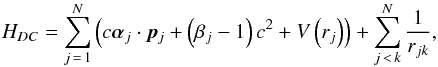 (2)where α and β are the Dirac matrices, p is the momentum operator, V(rj) is the monopole part of the electron-nucleus Coulomb interaction, and rjk is the distance between electrons j and k. The sums run over the number of electrons N. The angular integrations needed for the construction of the energy functional are based on second quantization in the coupled tensorial form 8; 9.
The Breit interaction ![\begin{eqnarray} \label{eq:Breit} H_{\mbox{{\footnotesize Breit}}} &=& - \sum_{j\,<\,k}^N \left[\; \boldsymbol{\alpha}_j \cdot \boldsymbol{\alpha}_k \; \frac{ \cos(\omega_{jk} r_{jk}/c)}{r_{jk}} \right. \nonumber \\ && \left. + \; (\boldsymbol{\alpha}_j \cdot \nabla_{j} ) \; (\boldsymbol{\alpha}_k \cdot \nabla_{k} ) \; \frac{ \cos(\omega_{jk}r_{jk}/c) -1}{\omega_{jk}^2 r_{jk}/c^2} \; \right] \end{eqnarray}](/articles/aa/full_html/2015/10/aa26708-15/aa26708-15-eq35.png) (3)and leading QED corrections (vacuum polarization and self-energy) are included in subsequent RCI calculations 21. In relativistic calculations, the states are given in jj-coupling. To adhere to the labeling conventions used by the experimentalists, the ASFs are transformed from the jj-coupling to the LS-coupling scheme using the methods developed by 10; 11. All calculations were performed with the GRASP2K code 16.
(3)and leading QED corrections (vacuum polarization and self-energy) are included in subsequent RCI calculations 21. In relativistic calculations, the states are given in jj-coupling. To adhere to the labeling conventions used by the experimentalists, the ASFs are transformed from the jj-coupling to the LS-coupling scheme using the methods developed by 10; 11. All calculations were performed with the GRASP2K code 16.
2.2. Computation of transition parameters
Transition parameters (transition probabilities A and oscillator strengths gf) for a transition between two states γ′P′J′M′ and γPJM can be expressed in terms reduced matrix elements 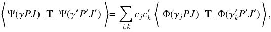 (4)where T is the transition operator. In cases where the initial and final state wave functions result from separate EOL calculations the wave functions are transformed in such a way that the orbital sets became biorthonormal 30 in which case standard methods can be used to evaluate the matrix elements between the CSFs.
For electric dipole (E1) and electric quadrupole (E2) transitions there are two forms of the transition operator, the length (Babushkin) form and the velocity (Coulomb) form. The length form is more sensitive to the outer parts of the wave functions and it is the preferred form. For RCI calculations the differences between the transition parameters evaluated with the two forms can be used as an indicator of the uncertainty 6. The quantity dT, characterizing the uncertainty of the computed transition rates, is defined as  (5)where Al and Av are transitions rates in length and velocity form.
2.3. Hyperfine structure
In atoms with nuclear spin I the fine-structure levels J are split into closely spaced hyperfine levels. The splittings of the fine-structure levels are to the first order given by the magnetic dipole AJ and electric quadrupole BJ hyperfine interaction constants 15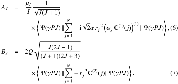 The hyperfine levels of closely spaced fine-structure levels are also affected by the off-diagonal hyperfine interaction 2. This effect is small, however, and is neglected in the present study. The calculations are done with the nuclear parameters I, μI, and Q all set to 1. To obtain the AJ and BJ values for a specific isotope, the given values should be scaled with the tabulated values of I, μI, and Q32.
Energy levels in cm-1 for the 15 lowest states in Fe XX as a function of increasing active sets of orbitals.
2.4. Landé gj-factors
The Landé gJ-factors are given by ![\begin{eqnarray} &&g_J = \frac{2}{\sqrt{J(J+1)}} \nonumber \\ && \times \left\langle \Psi(\gamma PJ) \| {\displaystyle \sum_{j\,=\,1}^N} \left[\! - \mbox{i} \frac{\sqrt{2}}{2\alpha^2} \, r_j \left( \boldsymbol{\alpha}_j {\bf C}^{(1)}(j) \right)^{(1)}\! +\! \frac{g_s-2}{2} \beta_j \boldsymbol{\Sigma}_j \!\right] \| \Psi(\gamma PJ)\right\rangle, \end{eqnarray}](/articles/aa/full_html/2015/10/aa26708-15/aa26708-15-eq81.png) (8)and determine the splitting of magnetic sublevels in external magnetic fields. Here gs is the electron g-factor and Σ the relativistic spin-matrix. The Landé gJ-factors were calculated using the Zeeman module of GRASP2K 1.
(8)and determine the splitting of magnetic sublevels in external magnetic fields. Here gs is the electron g-factor and Σ the relativistic spin-matrix. The Landé gJ-factors were calculated using the Zeeman module of GRASP2K 1.
Energy levels in cm-1 and the difference (Diff) between theoretical energies and observed Eobs.
2.5. Isotope shift
Isotope shift calculations using the MCDHF and RCI methods have recently been reviewed by Nazé et al. , and we refer to this paper for details. There are two contributions to the isotope shift: the mass shift and the field shift. For an atomic state γPJM the mass shift is expressed in terms of the normal  and specific
  mass shift parameters (in GHz u.):
  The field shift is the energy shift arising from the difference in nuclear charge distributions between two isotopes. The level field shift is given in terms of the
  parameter (in GHz/fm2), which is proportional to electron density at the origin
 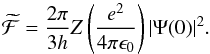 (11)The isotope shift parameters were calculated in the first-order perturbation approach using the RCI atomic state functions as zero-order wave functions. All calculations were done with the isotope shift module of GRASP2K 27.
3. Generation of configuration expansions
Separate calculations were performed in the EOL scheme for the 132 states of even parity and the 140 states of odd parity belonging to the 2s22p3, 2s2p4, 2p5, 2s22p23l, 2s2p33l, and 2p43l (l = 0,1,2) configurations. The CSF expansions were obtained using the active set method 29; 33. Defining the multireference (MR) as the CSFs that can be formed from, respectively, the even and odd parity configurations, the CSF expansions were generated from configurations obtained by single and double (SD) substitutions of the orbitals in the MR with orbitals in an active set with principal quantum numbers n = 3,...,8 (for Fe XX n = 3,...,9) and angular symmetries s,p,d,f,g, and h. Of the generated CSFs only those interacting with the CSFs of the MR were kept.
To monitor the convergence of the calculated energies and transition parameters, the active sets were increased in a systematic way by adding layers of orbitals. To reduce the number of CSFs in the self-consistent field calculations, the 1s2 core was closed from n = 6, but opened again in the subsequent RCI calculations. For the n = 8 expansion this resulted in 1 076 078 (6 206 696) CSFs with odd parity and 916 973 (5 255 680) CSFs with even parity with the 1s2 core closed (open). The self-consistent field calculations for each layer of orbitals were followed by RCI calculations, including the Breit interaction and the leading QED effects (vacuum polarization and self-energy).
4. Results
4.1. Fe XX
Computed energies of the 15 lowest states are given in Table 1 as functions of the increasing active orbital set. The mean relative difference between theory and experimental data from NIST is 1.32%, 1.21%, 0.58%, 0.21%, 0.08%, 0.09%, 0.05%, 0.04% for calculations based on the MR expansion and expansions obtained from SD substitutions to orbital sets with the highest principal quantum numbers n = 3,4,5,6,7,8,9. The calculations are well converged with respect to the increasing orbital set. A general observation is that the quartets states are energetically lower than the doublet states because electron correlation effects are smaller and converge faster with respect to the orbital set for high spin states than for low spin states 7; 12. The calculations do not quite manage to balance this. In Table 2 the current results are compared with results from other calculations. The current results and the results from Rynkun et al. and Gu stand out in a positive sense, with mean uncertainties of, respectively, 0.04%, 0.05%, and 0.04%. With the exception of the calculation by Vilkas & Ishikawa , the other calculations are associated with uncertainties that are larger by a factor of 10 or more. In Table 5 in the on-line material, calculated energies for all 272 states are compared with energies from Gu . There is perfect agreement; the two methods agree at the 0.025% level. There are a few experimental energies of 2s22p23d levels from NIST. Of these only half of them are validated by the calculations. Table 6 in the on-line material gives the energies, the AJ and BJ hyperfine constants, the Landé gJ factors, and the level mass- and field-shift parameters. Eigenvector compositions of the states in LSJ-coupling, which are used as labels, can be found on line in Table 7. LSJ-coupling is ideal for labeling and many of the states are heavily mixed.
Selected transition rates A are compared with rates from other calculations in Table 3. There is a detailed agreement with rates from Rynkun et al. , which is expected since the calculations are very similar. There is a good overall agreement between all calculated values. Table 14 in the on-line material contains transition energies, wavelengths, transition rates, weighted oscillator strengths, and uncertainty estimators dT for transitions between all 272 states. The uncertainty of the transition rates, as estimated by dT in Eq. (5), is around 1% for strong allowed transitions. For weak intercombination transitions the uncertainties are often larger. There are a number of weak two-electron one-photon transitions. These transitions are zero in the single configuration approximation and are allowed only through electron correlation effects. The two-electron one-photon transitions are known to be very difficult to compute and are associated with large uncertainties. From the transition rates the lifetimes of the states have been computed. The lifetimes in length and velocity form are given in Table 18. There is excellent agreement between the lifetimes in the two forms. There are, to the knowledge of the authors, no experimental lifetime data to compare with.
Comparison of transition rates: E1 transition rates between states of the upper (U) configuration 2s2p4 and the lower (L) configuration 2s22p3, E2 transition rates between states of the upper (U) configuration 2p5 and the lower (L) configuration 2s22p3, and M1 transition rates between states of 2s22p3 in Fe XX.
Energy levels in cm-1 and the difference (Diff) between theoretical energies and observed Eobs.
4.2. Cr XVIII, Ni XXII, and Zn XXIV
To reduce the computational effort the orbital sets were restricted to include orbitals with the highest principal quantum number n = 8. This will, based on the analysis of the convergence for Fe XX, only marginally affect the energies and transition rates. Energies of the 15 lowest states are given in Table 4. In the table, energies are compared with results from other calculations and with experimental energies from NIST. The mean relative energy differences between the present calculations and experimental data from NIST are 0.07%, 0.04%, and 0.04% for the three ions. The relative energy differences are of similar size for the calculations by Rynkun et al. and, for Ni XXII, by Gu . It is interesting to note that differences between the calculated and experimental energies for Zn XXIV do not follow the trends of the other ions. This may be due to the experimental conditions. When comparing with experimental data one should bear in mind that there are also experimental uncertainties that cannot be neglected.
Tables 8, 10, 12 in the on-line material give energies, AJ and BJ hyperfine constants, Landé gJ factors, and the mass- and field-shift parameters for all levels of Cr XVIII, Ni XXII, and Zn XXIV. Eigenvector compositions of the states of these ions are found in Tables 9, 11, and 13. There are basically no experimental data above the first 15 levels. The CHIANTI database gives energies for some higher lying states in Zn XXIV. These energies are, however, calculated and associated with large uncertainties. In addition, the given LSJ-labels disagree with the labels obtained from the present calculation. Transition energies, wavelengths, transition rates, weighted oscillator strengths, and uncertainty estimators dT for transitions between all 272 states are available on line in Tables 15−17. Lifetimes in length and velocity form are given in Tables 19−21. The uncertainties estimated from dT are similar to the values for Fe XX. The mean relative difference between the lifetimes in the length and velocity form is around 2.5%0 for the three ions.
4.3. Summary and conclusions
Self-consistent MCDHF and subsequent RCI calculations were performed for the nitrogen-like ions Cr XVIII, Fe XX, Ni XXII, and Zn XXIV using GRASP2K. Energies, AJ and BJ hyperfine constants, Landé gJ-factors, mass- and field-shift parameters, and transition rates involving the 2s22p3, 2s2p4, 2p5, 2s22p23l, 2s2p33l, and 2p43l (l = 0,1,2) configurations are given. Compositions of atomic state functions in LSJ-coupling are also reported. Previous theoretical and experimental data for Fe XX were used to validate computational methods. Energies from the RCI calculations are in excellent agreement with observations. For the 15 lowest states the mean relative energy differences are around 0.04% (NIST Atomic Spectra Database 2013) for the four ions. This translates to wavelengths that are accurate to within ± 10 mÅ and thus of spectroscopic accuracy. The high accuracy carries over also to the higher states.
Uncertainties in electric dipole transition rates between the lower states have been estimated from the expressions suggested by Ekman et al. giving an average of only 1.9%. We thus argue that the transition rates are highly accurate and may serve as benchmarks for other calculations. To summarize, the present work has significantly increased the amount of accurate data for ions in the nitrogen-like sequence.
Acknowledgments
The authors are thankful for the high performance computing resources provided by the Information Technology Open Access Center of Vilnius University.
References
- Andersson, M., & Jönsson, P. 2008, Comput. Phys. Commun., 178, 156 [NASA ADS] [CrossRef] [Google Scholar]
- Andersson, M., Jönsson, P., & Sabel, H. 2006, J. Phys. B, 39, 4239 [NASA ADS] [CrossRef] [Google Scholar]
- Bhatia, A. K., Seely, J. F., & Feldman, U. 1989, At. Data Nucl. Data Tables, 43, 99 [NASA ADS] [CrossRef] [Google Scholar]
- Dyall, K. G., Grant, I. P., Johnson, C. T., Parpia, F. A., & Plummer, E. P. 1989, Comput. Phys. Commun., 55, 425 [NASA ADS] [CrossRef] [Google Scholar]
- Ekman, J., Godefroid, M., & Hartman, H. 2014a, Atoms, 2, 215 [NASA ADS] [CrossRef] [Google Scholar]
- Ekman, J., Jönsson, P., Gustafsson, S., et al. 2014b, A&A, 564, A24 [NASA ADS] [CrossRef] [EDP Sciences] [Google Scholar]
- Froese Fischer, C., Brage, T., & Jönsson, P. 1997, Computational Atomic Structure (Bristol and Philadelphia: Institute of Physics Publishing) [Google Scholar]
- Gaigalas, G., Rudzikas, Z., & Froese Fischer, C. 1997, J. Phys. B: At. Mol. Opt. Phys., 30, 3747 [Google Scholar]
- Gaigalas, G., Fritzsche, S., & Grant, I. P. 2001, Comput. Phys. Commun., 139, 263 [NASA ADS] [CrossRef] [Google Scholar]
- Gaigalas, G., Žalandauskas, T., & Rudzikas, Z. 2003, At. Data Nucl. Data Tables, 84, 99 [NASA ADS] [CrossRef] [Google Scholar]
- Gaigalas, G., Žalandauskas, T., & Fritzsche, S. 2004, Comput. Phys. Commun., 157, 239 [NASA ADS] [CrossRef] [Google Scholar]
- Galvez, F. J., Buendia, E., & Sarsa, A. 2005, J. Chem. Phys., 123, 034302 [NASA ADS] [CrossRef] [Google Scholar]
- Gu, M. F. 2005, ApJSS, 156, 105 [NASA ADS] [CrossRef] [Google Scholar]
- Jonauskas, V., Bogdanovich, P., Keenan, F. P., et al. 2005, A&A, 433, 745 [NASA ADS] [CrossRef] [EDP Sciences] [Google Scholar]
- Jönsson, P., Parpia, F.A., & Fischer, F. C. 1996, Comput. Phys. Commun., 96, 301 [NASA ADS] [CrossRef] [Google Scholar]
- Jönsson, P., Gaigalas, G., Bieroń, J., Froese Fischer, C., & Grant, I. P. 2013, Comput. Phys. Commun., 184, 2197 [NASA ADS] [CrossRef] [Google Scholar]
- Kotochigova, S., Linnik, M., Kirby, K. P., & Brickhouse, N. S. 2010, ApJSS, 186, 85 [NASA ADS] [CrossRef] [Google Scholar]
- Kramida, A., Ralchenko, Yu., Reader, J., & NIST ASD Team 2012. NIST Atomic Spectra Database, ver. 5.0 (Online), available: http://physics.nist.gov/asd (2013, May 30), National Institute of Standards and Technology, Gaithersburg, MD [Google Scholar]
- Lemaire, P., Wilhelm, K., & Curdt, W., et al. 1997, Sol. Phys., 170, 105 [NASA ADS] [CrossRef] [Google Scholar]
- Lepson, J. K., Beiersdorfer, P., Clementson, J., et al. 2010, J. Phys. B: At. Mol. Opt. Phys., 43, 144018 [NASA ADS] [CrossRef] [Google Scholar]
- McKenzie, B. J., Grant, I. P., & Norrington, P. H. 1980, Comput. Phys. Commun., 21, 233 [NASA ADS] [CrossRef] [Google Scholar]
- Merkelis, G., Vilkas, M. J., Kisielius, R., & Gaigalas, G. 1997, Phys. Scr., 56, 41 [NASA ADS] [CrossRef] [Google Scholar]
- Merkelis, G., Martinson, I., Kisielius, R., & Vilkas, M. J. 1999, Phys. Scr., 59, 122 [NASA ADS] [CrossRef] [Google Scholar]
- Mewe, R., Raassen, A. J. J., & Drake, J. J., et al. 2001, A&A, 368, 888 [NASA ADS] [CrossRef] [EDP Sciences] [Google Scholar]
- Mewe, R., Raassen, A., J., J., & Cassinelli, J. P., et al. 2003, A&A, 398, 203 [NASA ADS] [CrossRef] [EDP Sciences] [Google Scholar]
- Nahar, S. N. 2004, A&A, 413, 779 [NASA ADS] [CrossRef] [EDP Sciences] [Google Scholar]
- Nazé, C., Gaidamauskas, E., Gaigalas, G., Godefroid, M., & Jönsson, P. 2013, Comput. Phys. Commun., 100, 1197 [Google Scholar]
- Nazé, C., Verdebout, S., Rynkun, P., et al. 2014, At. Data Nucl. Data Tables, 184, 2187 [Google Scholar]
- Olsen, J., Roos, B. O., Jorgensen, P., & Jensen, H. J. Aa. 1988, J. Chem. Phys., 89, 2185 [NASA ADS] [CrossRef] [Google Scholar]
- Olsen, J., Godefroid, M., Jönsson, P., Malmqvist, P. Å., & Froese Fischer, C. 1995, Phys. Rev. E, 52, 4499 [NASA ADS] [CrossRef] [Google Scholar]
- Rynkun, P., Jönsson, P., Gaigalas, G., & Froese Fischer, C. 2014, At. Data Nucl. Data Tables, 100, 315 [NASA ADS] [CrossRef] [Google Scholar]
- Stone, N. J. 2005, At. Data and Nucl. Data Tables, 90, 75 [Google Scholar]
- Sturesson, L., Jönsson, P., & Fischer, C. F. 2007, Comput. Phys. Commun., 177, 539 [NASA ADS] [CrossRef] [Google Scholar]
- van der Heyden, K. J., Bleeker, J. A. M., Kaastra, J. S., & Vink, J. 2003, A&A, 406, 141 [NASA ADS] [CrossRef] [EDP Sciences] [Google Scholar]
- Vilkas, M. J., & Ishikawa, Y. 2001, Adv. Quant. Chem., 261, 39 [Google Scholar]
- Wilhelm, K., Lemaire, P., Curdt, W., et al. 1997, Sol. Phys., 170, 75 [NASA ADS] [CrossRef] [Google Scholar]
All Tables
Energy levels in cm-1 for the 15 lowest states in Fe XX as a function of increasing active sets of orbitals.
Energy levels in cm-1 and the difference (Diff) between theoretical energies and observed Eobs.
Comparison of transition rates: E1 transition rates between states of the upper (U) configuration 2s2p4 and the lower (L) configuration 2s22p3, E2 transition rates between states of the upper (U) configuration 2p5 and the lower (L) configuration 2s22p3, and M1 transition rates between states of 2s22p3 in Fe XX.
Energy levels in cm-1 and the difference (Diff) between theoretical energies and observed Eobs.
Current usage metrics show cumulative count of Article Views (full-text article views including HTML views, PDF and ePub downloads, according to the available data) and Abstracts Views on Vision4Press platform.
Data correspond to usage on the plateform after 2015. The current usage metrics is available 48-96 hours after online publication and is updated daily on week days.
Initial download of the metrics may take a while.